Climate Change and Grain Price Volatility: Empirical Evidence for Corn and Wheat 1971–2019

Abstract

It is widely recognized that climate change makes the weather more erratic. As the combination of temperature and precipitation is a major driver of grain crop productivity, more frequent extreme rainfalls and heat waves, flooding and drought tend to make grain production and hence grain prices more volatile. We analyze daily prices during the growing season for corn and wheat over the period 1971–2019 using an EGARCH model. There have been occasional spikes in price volatility throughout this period. We do not, however, find that grain prices have become more volatile since the 1970s, with an exception for a small but statistically significant upward trend in wheat price volatility. To the extent that climate change has caused more frequent weather extremes affecting crop yields, it appears that the price effects have been softened, most likely through farmers’ adaption to climate changes, introduction of more stress-tolerant hybrids, storage, regional and international trade and risk management instruments.

1. Introduction

Farmers who see their crops greatly reduced or ruined by unfavorable weather conditions, such as extreme heat and too much or too little rain, is nothing new. What is new, however, is the fact that climate change may trigger crop failures more frequently and on a larger scale. There is a wide consensus that the global climate has changed over the past decades causing a more erratic environment for agricultural production (IPCC [1,2]). While adverse weather conditions and crop failures in one geographical area often have been compensated by favorable weather and bumper crops in other areas, climate change may have an increasingly negative impact on yields over large areas (Kopp et al. [3], Tigchelaar et al. [4]). Climate change substitutes systematic global risk for idiosyncratic, unsystematic local or regional risk.

While there is disagreement about the magnitude (and even the direction) of the impact that climate change will have on global food production, there has been a growing concern that we may see dramatic negative effects on food production in large geographical areas to the extent that global food security may be at risk. Based on a significant number of studies, IPCC [1] (p. 996) concludes that “Over the past several decades, observed climate trends have adversely affected wheat and maize production for many regions, as well as the total production of these crops”. Ortiz-Bobea et al. [5] in their analysis of agricultural total factor productivity conclude that climate change has slowed global productivity growth by some 20% since 1960. As documented in several studies, increased variations in precipitation will increase variability in wheat yields in major production areas unless new management practices are adapted (Hatfield and Dold [6]). Projected increases in temperature, reductions in precipitation, and increased frequency of extreme events may result in net productivity declines in major North American crops at a scale that would affect global food supply and hence cause increased volatility in world prices (Huchet-Bourdon [7], Ray et al. [8]).

Higher food price volatility increases uncertainty for food producers, distributors and the agribusiness sector. Further, food price volatility is important from a public policy perspective as it affects people’s ability to purchase food, especially the world’s poorest. Understanding volatility is also important to consumers and for policy making (Musunuru [9]).

In their much quoted study, Gilbert and Morgan [10] found that food price volatility generally had been lower during the period 1990–2010 than during the previous decades, despite the price spikes in 2008. Regarding grains, they found that price volatility for corn and soy beans fell significantly between 1970 and 2009, while there was an insignificant rise in wheat price volatility. Rice stood out as an exception with a significant volatility rise. Their findings are in line with those of Balcombe [11] who failed to find evidence of any general increase in food price volatility. Gilbert and Mugera [12], however, using daily data for the period 2000–2011, reported increasing volatility over this time period. In addition, Dawson [13] found evidence of increased volatility in daily wheat prices using data from 1996–2012. In their conclusion, Gilbert and Morgan [10] suggested that grain price volatility might increase in the future due to factors, such as global warming and oil price volatility transmitted via biofuel demand.

The purpose of this paper is to assess whether the price volatility for agricultural products has increased over time. The underlying hypothesis is that increasingly erratic weather caused by, say climatic change, has increased market risk as reflected in more volatile prices. Thus, this study is not about agricultural price levels but about price volatility. More precisely, we test if there are any observable long-term trends in price volatility.

This paper adds to the existing literature in two ways. For one, we update the data sample used in previous seminal studies by Gilbert and Morgan [10], Gilbert and Mugera [12] and Dawson [13]. Extending the sample period both prior to and beyond the price spikes observed in 2008 adds to the understanding and robustness of any claims about trends in price volatility.

Second, we suggest a methodological approach that is somewhat different to the one used in most previous studies. Our approach is in a similar vein as the one applied by Musunuru [9] to examine volatility persistence and news asymmetry in soybean futures returns. However, Musunuru [9] studied short-term volatility characteristics; we focus on long-term trends in volatility.

We analyze the long-term development in volatility in daily changes in futures prices for two key crops, corn and wheat, using a heteroskedastic EGARCH model with a linear trend in the volatility (Pindyck [14]). The underlying hypothesis is that increasingly erratic weather caused by, say climatic change, has increased market risk as reflected by price volatility. In order to catch market reactions to actual weather events as well as expectations regarding future yields, we use daily futures prices. The futures market is generally the arena where news is immediately integrated into price changes. Observing prices at a daily frequency enables us to analyze the immediate market effects from relevant weather information and dramatic events having an impact on expected yields. Roll [15] found that the daily price of frozen orange juice concentrate is affected by cold temperature and that returns on orange juice have a statistically significant relation with subsequent errors in temperature forecasts. Using prices observed at lower frequencies, say monthly or quarterly, as is the case in most past studies, will easily dampen the effects from a more erratic weather pattern.

This paper is organized as follows. In the next section, we survey major contributions to the scientific debate on the effects from climate change on production and prices. We then proceed to present the price data used in our analysis as well as a brief description of global production and productivity growth for wheat and corn 1970–2019 before outlining the econometric model and results. Section 6 summarizes our main conclusions.

2. Climate Change, Food Production and Prices

There is a large and growing body of literature on the possible effects of climate changes on food production and food prices. As stated in the introduction, Ortiz-Bobea et al. [5] concluded that climate change has slowed global productivity growth in agriculture by some 20% during the last 60 years. Deschênes and Greenstone [16] argued that the long-term effect of global warming on production of US corn and soybean yields is limited, or perhaps even positive. Fisher et al. [17], using the same (but corrected) data set as Deschênes and Greenstone [16], concluded that global warming is likely to have negative long-term effects on yields.

Ray et al. [8] studied how climate affects crop variations in many geographical regions. Based on a relatively simple model where temperature and precipitation represent the climate variables, the annual deviations from the long-term trend in crop per hectare were estimated over the period 1979–2008. They found that, overall, climate variation explains one-third of global crop yield variability for maize, rice, wheat and soybeans. While some areas show no significant influence of climate variability, the study concluded that in important cereal production regions more than 60 percent of yield variability can be explained by climate variability. The results lend support to an earlier study by Schlenker and Roberts [18], who found a strong relationship between corn, soybean and cotton yields and weather, predicting yield losses of 30–46 percent by the end of the century under the slowest warming scenario and substantially more under the fastest warming scenario.

However, climate changes may have opposite effects across different regions. Thus, Kucharik and Serbin [19], focusing on Wisconsin on the northern, cooler fringes of the US corn belt, found that a warmer climate could help support higher corn and soybean yields and that trends in precipitation and temperature during the growing season from 1976 to 2006 explained 40 percent and 35 percent of county corn and soybean yield trends, respectively. On a global scale, Lobell and Field [20] found that growing season temperatures and precipitation–spatial averages based on the locations of each crop explain some 30 percent or more of year-to-year variations in global average yields for the world’s six most widely grown crops. They concluded that for the major grains, there is a clearly negative response of global yields to increased temperatures and that global warming in the period 1981–2002 resulted in annual combined losses (wheat, maize and barley) of roughly 40 million tons. Although this signified a relatively small impact compared to the technological yield gains, they concluded that by 2002 these results already demonstrated that climate change had negative impacts on crop yields on a global scale.

Marginal changes in temperature may have severe impact on yields. In a large econometric study covering corn and soybeans, i.e., the two largest food crops in the United States, Schlenker and Roberts [18] found that yields increase linearly in temperatures up to 29 °C for corn and 30 °C for soybeans. Above that level, temperature increases become harmful. Thus, there seems to be strong nonlinear temperature effects on yields (Schlenker et al. [21], Lobell et al. [22]), implying that marginal changes in temperature (as well as precipitation) may have significant effects on yields and hence supply and food prices.

In the longer run, producers may adapt to climatic changes by, e.g., developing and introducing more heat- or drought-tolerant varieties and improving storage management. The effects from regional extreme weather events may furthermore be cushioned through extensive and diversified inter-regional and international trade. However, in the short run, i.e., within the growing season, we would expect to find a higher frequency of extreme price movements due to more extreme weather conditions over the last 2–4 decades.

3. Data and Descriptive Statistics

Price data consist of daily December futures contracts (opening prices) for corn and wheat from the Chicago Mercantile Exchange (CME), collected from Bloomberg. We created continuous series using 1 November as the rollover date. Nominal contract prices were converted to real prices using the annual consumer price index (with 2015 as the base year) for all prices belonging to the December contract of the corresponding year. Log returns were calculated, and returns on the rollover date were removed. Production data were collected from FAOSTAT.

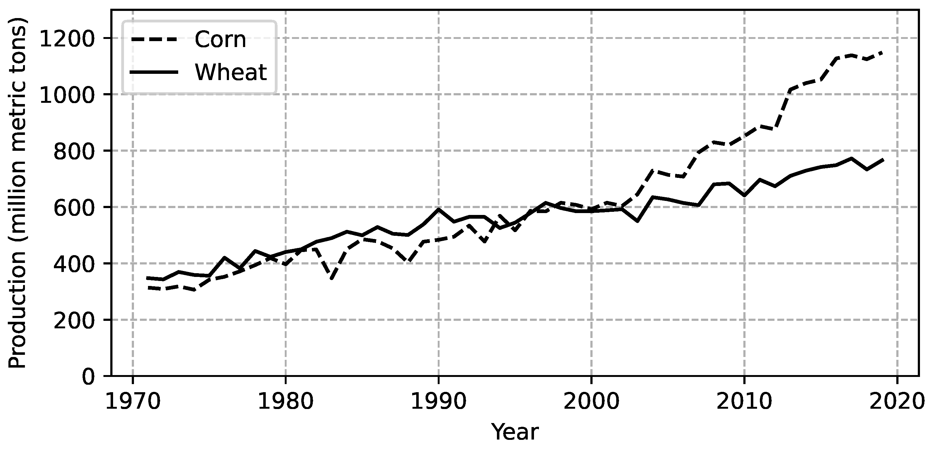
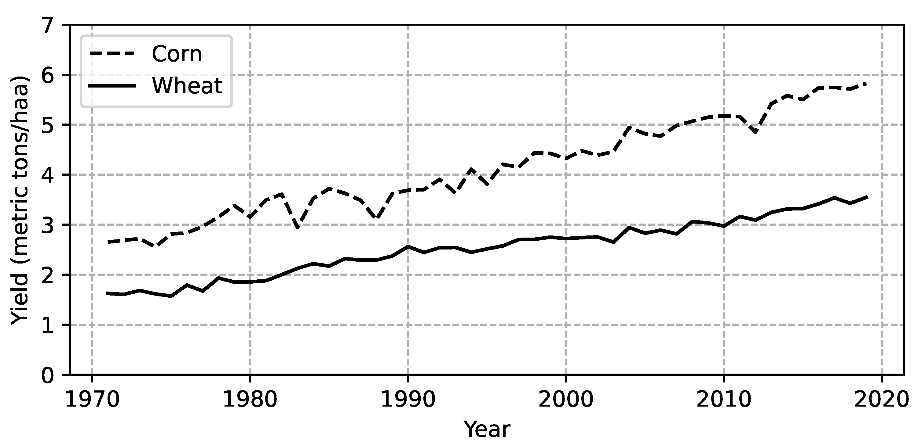
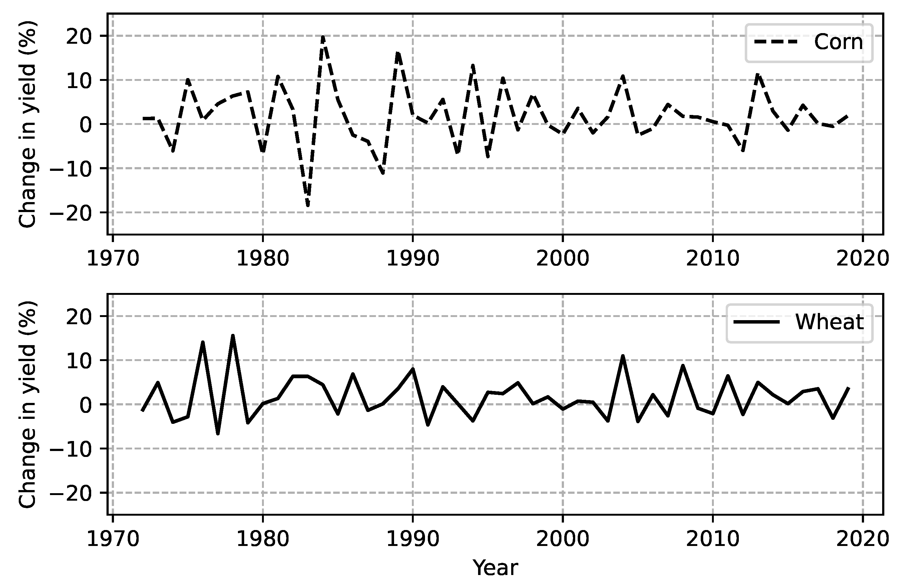
3.1. Global Wheat and Corn Production 1971–2019

There has been substantial growth in world production of both wheat and corn over the past five decades. In 1971, world production was roughly 348 million and 314 million metric tonnes (MT) for wheat and corn, respectively (Figure 1). By the turn of the millennium, total production had grown in tandem, approaching 600 million MT for both wheat and corn. Over the next two decades, corn production outpaced that of wheat by far, reaching almost 1.150 million MT compared to 766 million MT for wheat. Long-term annual growth over the past five decades was 1.5 percent for wheat and 2.8 percent for corn. Over the last two decades, corn production grew by 3.7 percent annually.

Production growth has two sources, i.e., higher yields, and/or larger acreage. Focusing on total production, adverse climatic conditions do not seem to be reflected in the graphs in that we see no clear breaks and trend changes. Part of the steady long-term growth is due to more land being tilled, as for instance the farming of huge new areas in the cerrado (savannah) in Brazil. However, the major driver behind the growth is clearly to be found in science (higher yielding varieties) and improved agronomic practices. This is visualized in Figure 2, showing that globally, yields (kilo per hectare) more than doubled between 1971 and 2019 for both wheat and corn. Thus, in the 1970s, average production was around 1600–1800 kilos/ha for wheat and some 2600–3300 kilos for corn. By 2019, average yields had risen to more than 3500 kilos for wheat and 5800 kilos for corn.

Yields are driven by technological development, such as the introduction of new and better varieties, more efficient chemicals when it comes to combating weeds, fungi and pests and improved competence among farmers. Yield variations are also driven by changes in input prices causing farmers to reduce or increase their application of fertilizers or other chemicals. Likewise, yields may change as a result of moving in or out of more or less productive environments, and changes in agronomic practices may cause both short-term and long-term variations in yields. In the short-term, however, there is reason to assume that crop variations are primarily driven by variations in regional weather conditions and in the longer term by global changes in climate. Looking beyond the long-term trend, climate change is more likely reflected in short-term yield variations as a result of more frequent severe droughts, extreme temperatures, etc., in important larger grain producing areas. Despite the fact that there has been strong growth in corn and wheat yields globally over the past 50 years, one would expect to find larger short-term yield variations driven by increasingly more erratic weather. Figure 3 suggests that this has not been the case. On the contrary, yields have both increased and become less volatile after 2000 compared to the period 1971–1996. This may suggest that the negative effects from climate change have been damped by science, farmers and functioning markets.

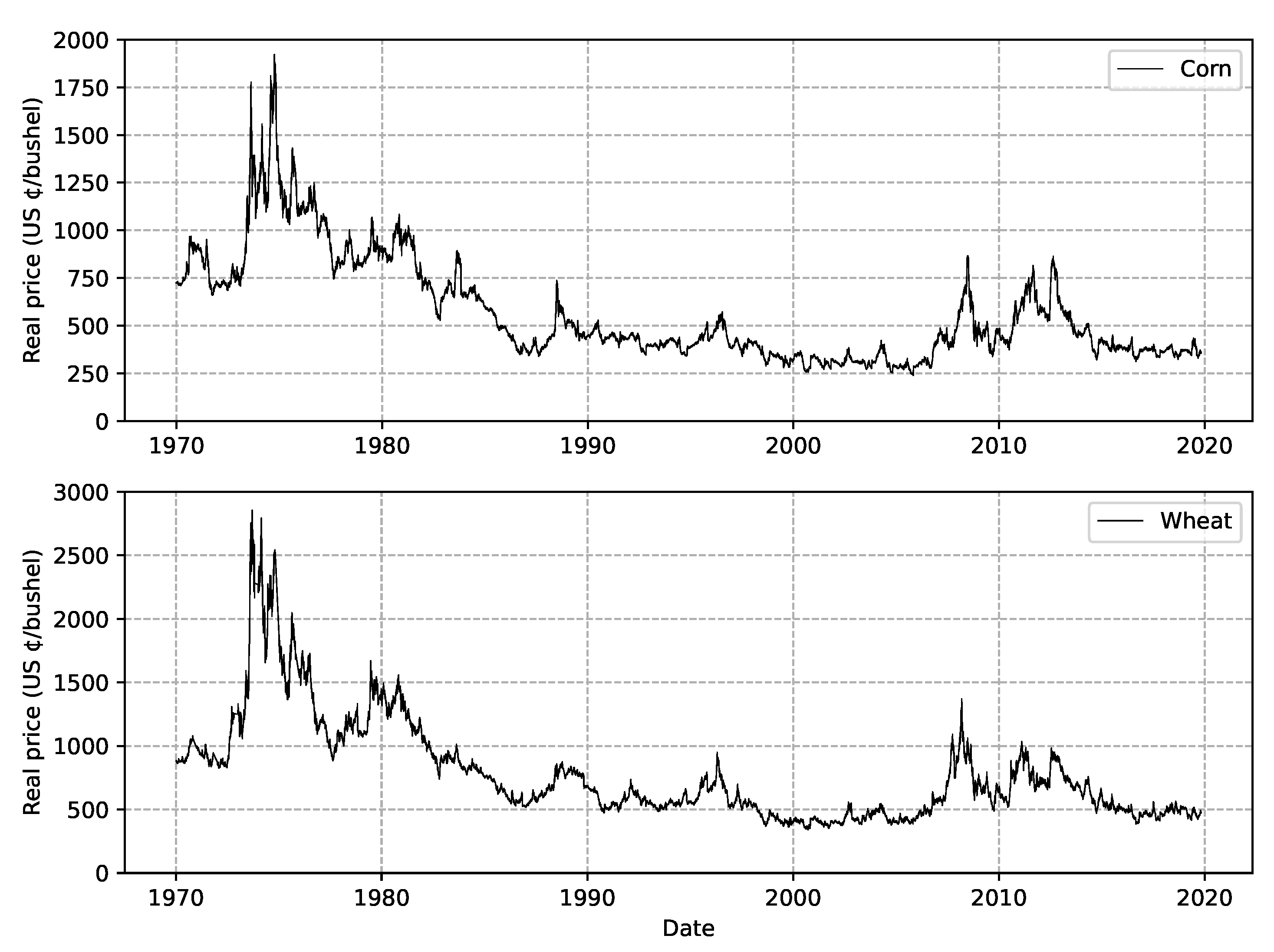
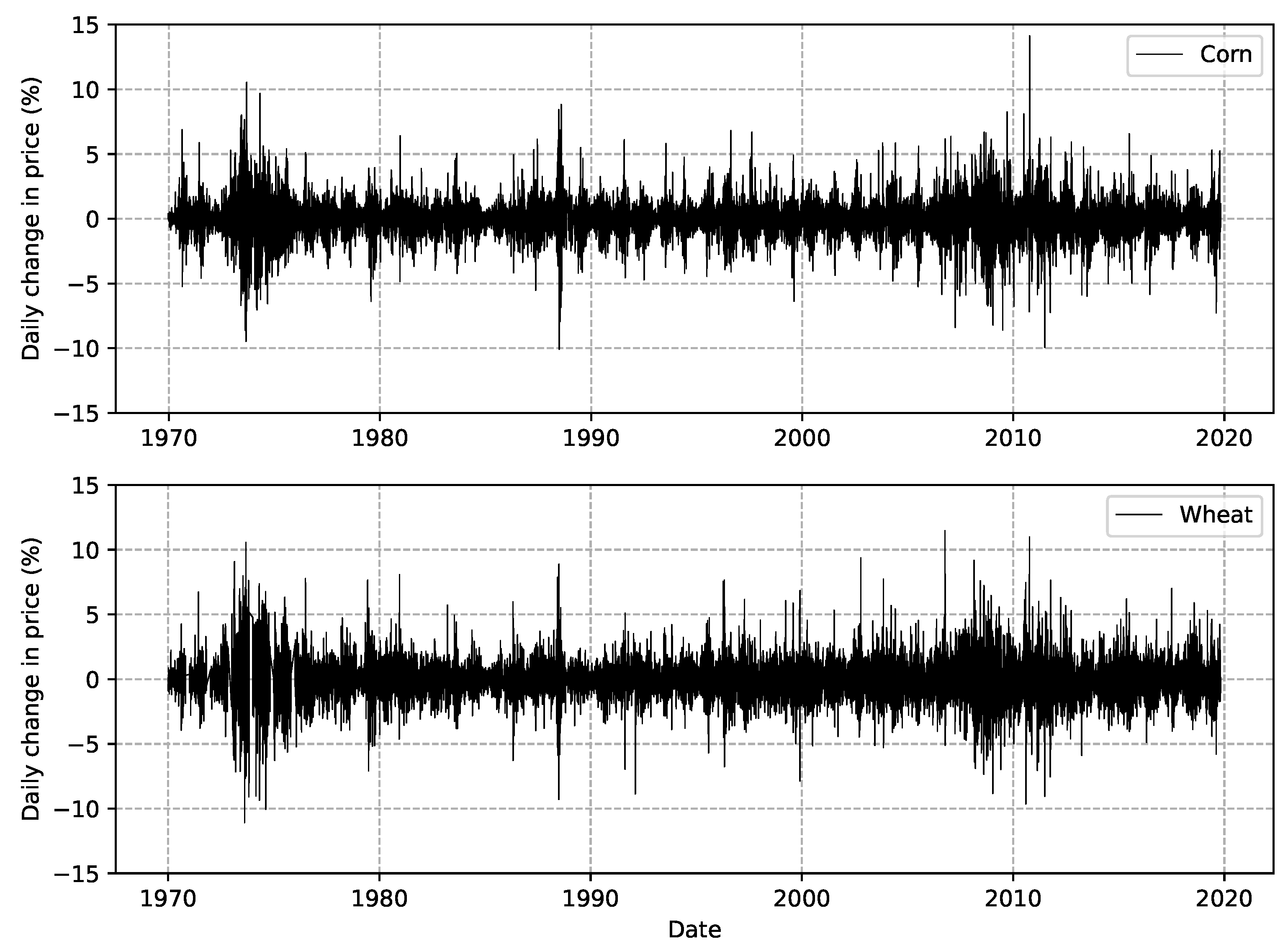
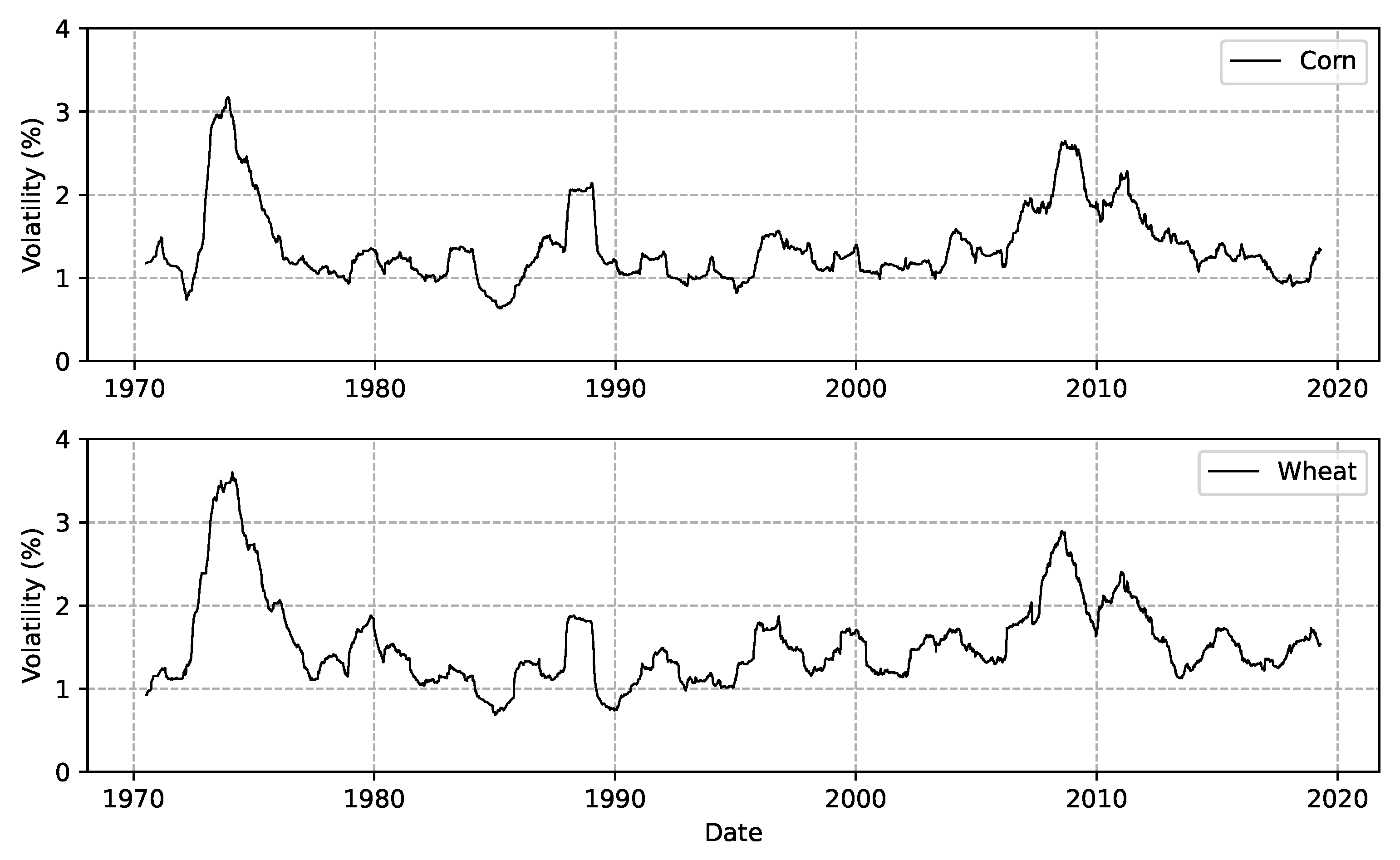
3.2. Prices and Volatility

Figure 4 show deflated price series for corn and wheat. Both prices rose substantially during the 1970s. This was the case for most commodities and was due to several reasons. Since the end of the 1970s, real commodity prices fell steadily until early 2000. Since then, we see a slight, then a sharp increase into the next boom and bust, the so called “Food Crisis”. There has been a major debate over causes of this boom and bust. That debate, however, is not the focus of this paper. For a detailed analysis of the boom and bust in the 1970s as well as the one in 2008, see, e.g., Carter et al. [23]. Since around 2012, grain prices have settled down. We are not including any developments after the period covered here, i.e., the COVID-19 pandemic and the war in Ukraine.

The volatility in the grain prices are evident in Figure 5 showing daily price changes and in Figure 6 showing the standard deviation of the price changes over a rolling window covering 275 trading days. The contracts are typically traded for 260 or 261 days. The rolling window will always cover more than one contract. The period of higher prices in 2007–2013 are accompanied by higher price volatility. Some considered this a warning of something even more volatile to come. So far, this prediction has not materialized, and volatility has returned to levels similar to that of the 1990s.

3.3. Descriptive Statistics

Table 1. Summary statistics for real futures prices for corn and wheat, 1970–2019.

	Corn		Wheat
	Real Price	Change in Price (%)	Real Price	Change in Price (%)
Mean	301.28	−0.010	416.74	−0.003
Standard deviation	115.66	1.442	159.11	1.598
Minimum	112.63	−10.069	141.37	−11.081
Median	267.50	0.000	373.50	0.000
Maximum	837.50	14.122	1245.00	11.463
Skewness		0.110		0.135
Kurtosis (Fisher)		5.129		4.028
KPSS-test		0.14		0.25
Ljung-Box Q(5)		23.61		82.10
ARCH(1) test		397.99		531.23
Observations	12936		12658

presents the summary statistics for the real futures contract prices and changes in these expressed as day-over-day percent changes, or returns. The average price change is negative for both crops, reflecting a long-term decline in real prices as evident from Figure 4. The volatility in the prices expressed as the sample standard deviation is about 1.4% and 1.6% for corn and wheat, respectively.

The skewness of both price change series is low. indicating close to symmetric distributions for both crops. The high kurtosis indicates that the distributions are leptokurtic with fatter tails than a normal distribution. The low values for the KPSS test statistics confirm that the series are stationary. The KPSS statistics for corn and wheat have 14 and 8 lags, respectively, and p-values of 0.1. and the high values of the Ljung-Box statistics mean that there is substantial autocorrelation in the series.

4. Empirical Framework

The pattern of the price changes in Figure 5 is indicative of periodic volatility clustering, and such persistent volatility is well documented in past studies (Balcombe [11], Gilbert and Mugera [12], Dawson [13]). Thus, an autoregressive conditional heteroskedasticity (ARCH) model may be appropriate. The results of a Lagrange Multiplier test of Engle [24] for an ARCH model, see Table 1, clearly rejects the null hypothesis of homoskedasticity of the returns. The generalized ARCH (GARCH) model proposed by Bollerslev [25] allows the conditional variance to follow an autoregressive moving average (ARMA) process. The exponential generalized ARCH (EGARCH) model of Nelson [26] allows for asymmetry in the impact of shocks on the volatility of the returns. Musunuru [9] found clear evidence of asymmetry in his empirical analysis of soybean futures returns, a finding which is consistent across different asymmetric GARCH models.

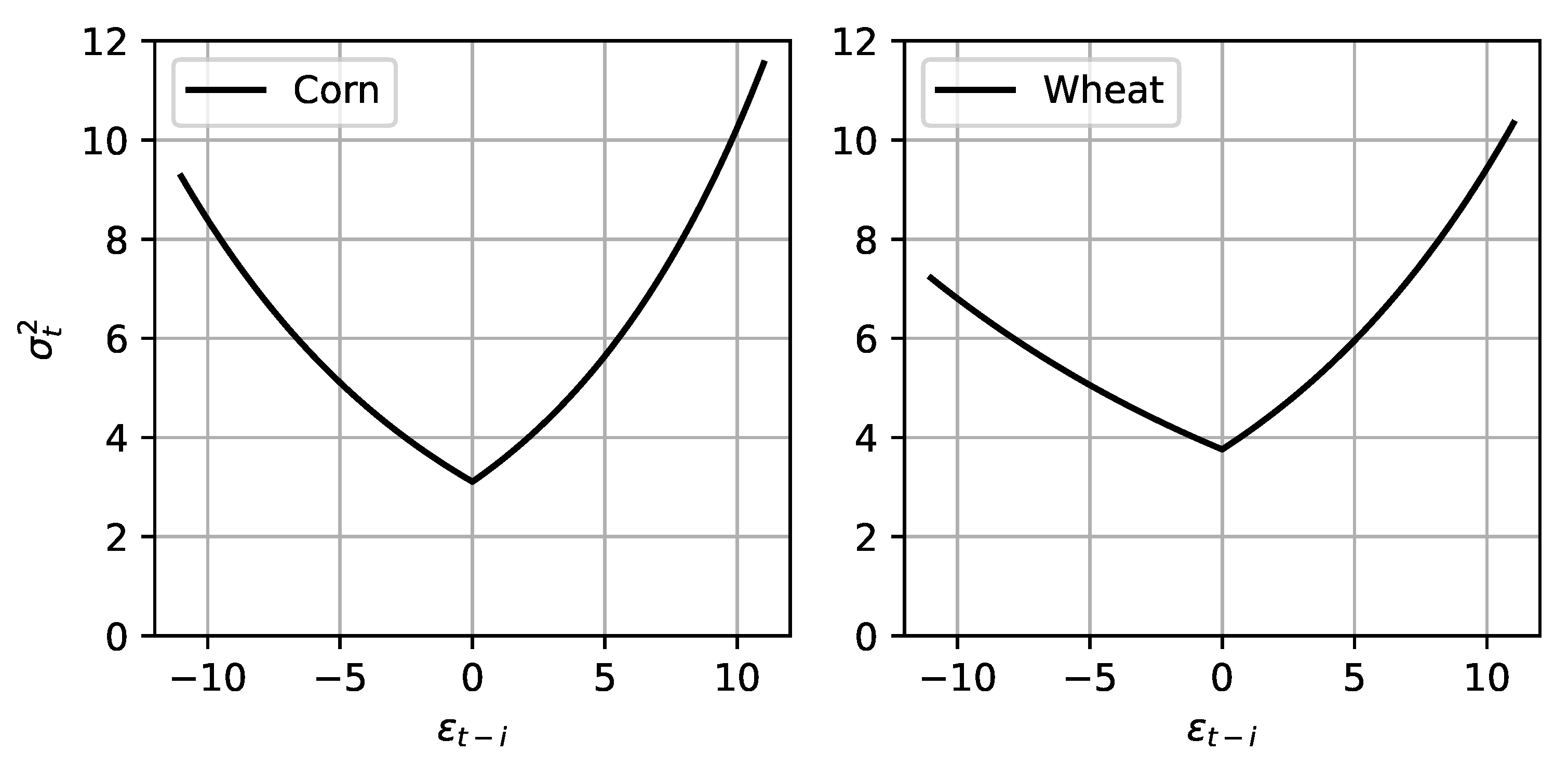
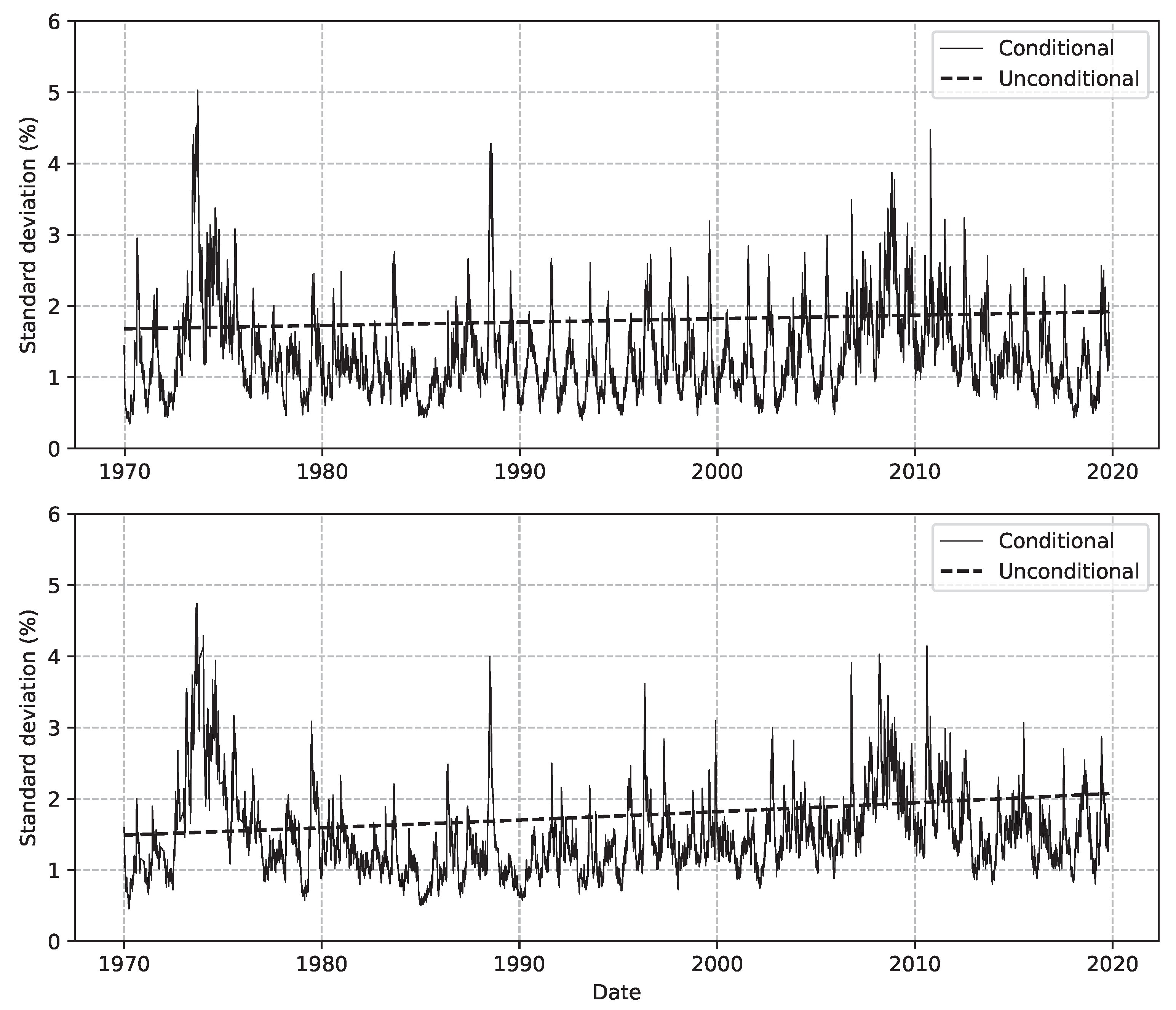
Heterogeneous EGARCH Model

The EGARCH model for returns, $r_t$ at time t, with heterogeneous variance is specified as:

$$\begin{array}{cc}\hfill r_t& =\mu +\sum _{i=1}^s{\psi }_i{r}_{t-i}+{\epsilon }_t\hfill \end{array}$$

(1)

$$\begin{array}{cc}\hfill {\epsilon }_t& ={\sigma }_t{\nu }_t,{\nu }_t\sim iid(0,1)\hfill \end{array}$$

(2)

$$\begin{array}{cc}\hfill ln\left({\sigma }_t^2\right)& =\omega +\delta T_t+\sum _{i=1}^p{\beta }_{i}ln\left({\sigma }_{t-i}^2\right)+\sum _{i=1}^q\left[{\gamma }_i{z}_{t-i}+{\alpha }_i\left(|z_{t-i}|-E(|z_{t-i}\left|\right)\right)\right]\hfill \end{array}$$

(3)

where

$$z_{t-i}=\frac{{\epsilon }_{t-i}}{\sqrt{{\sigma }_{t-i}^2}}.$$

and ${\nu }_t$ are shocks with zero mean and unit variance.

Here, Equation (1) is an autoregressive (AR) model with s lags for the returns. Equations (2) and (3) define the ARCH components of the model with p EGARCH terms and q EARCH terms.

The high kurtosis found for the price changes for both corn and wheat implies that the distributions for price changes are highly leptokurtic. Following [27], we estimate the model using maximum likelihood methods under the assumption that ${\nu }_t$ has a student t-distribution with mean zero and f degrees of freedom where f is to be estimated.

The inclusion of a time trend $T_t$ in Equation (3) makes the variance (volatility) heterogeneous over time. The trend variable $T_t$ is defined such that it increases 1/365.25 for each calendar day. Thus, $\delta$ represents an annual rate of change. This specification of the conditional variance equation allows us to statistically test for a linear time trend in volatility (Pindyck [14]). If the volatility in the crop prices have increased over time, the parameter $\delta$ should be positive and statistically significant.

5. Results and Discussion

The parameters of the EGARCH model are estimated using maximum likelihood techniques and are reported in

Table 2. Estimated EGARCH models for corn and wheat daily returns.

Parameter	Corn	Wheat
$\mu$	−0.01166	−0.01127
	(0.00787)	(0.00938)
${\psi }_1$	−0.03164	−0.06195
	(0.00704)	(0.00863)
${\psi }_2$	−0.03008	−0.02510
	(0.00956)	(0.00997)
$\omega$	0.01380	0.01011
	(0.00313)	(0.00258)
$\delta$	0.71 × 10${}^{-4}$	1.71 × 10${}^{-4}$
	(0.99 × 10${}^{-4}$)	(0.81 × 10${}^{-4}$)
${\beta }_1$	0.98666	0.98713
	(0.00181)	(0.00189)
${\gamma }_1$	0.01917	0.03370
	(0.00585)	(0.00544)
${\alpha }_1$	0.20943	0.15598
	(0.01811)	(0.00979)
f	6.2966	7.4571
	(0.3491)	(0.4752)
N	12,936	12,658

Robust standard errors in paranthesis.

, along with robust standard errors. The length of the AR term was chosen to minimize the Akaike Information Criteria. The models for both crops include one EARCH and one EGARCH term. Adding additional EARCH and/or EGARCH terms to the model did not improve AIC.

The EGARCH parameter ${\beta }_1$ measures the persistence in conditional volatility. The estimate value of this parameter is 0.987 for both corn and wheat. This high value implies that shocks will persist in the volatility for a long time with a half life of 52 and 54 trading days, respectively.

The EGARCH model allows for asymmetry in the response in volatility to positive and negative shocks through the parameter ${\gamma }_1$. This parameter is positive and significant for both crops. The positive sign implies that positive shocks will have a greater impact on volatility compared to a negative shock. The news impact curve of Engle and Ng [28] can be used to illustrate the asymmetry in the response. Figure 7 evaluates the impact of shocks in one period on the variance in the next period where the baseline is the unconditional variance. The impact of similar shocks on volatility are greater for corn than wheat. The response is greater for positive shocks than negative shocks. This is consistent with the finding by Musunuru [9] for soybean futures.

Our key parameter is the time trend coefficient $\delta$ which has positive parameter estimates for both crops. This parameter is not statistically different from zero in the model for corn with a z-value of 0.72. On the other hand, the z-value is 2.11 for wheat. Thus, there is no change in the volatility of futures prices for corn, while there is a statistically significant but quite small increase in volatility for wheat.

This result supports the findings of Lybbert et al. [29] that wheat is grown mainly in the northern hemisphere and therefore is more vulnerable to climate change compared to corn where production is more evenly distributed between northern and southern hemispheres. Thus, the potential for a rapid supply response to price changes is greater for corn than for wheat.

The sample standard deviations for price changes are 1.4% and 1.6% for corn and wheat, respectively. Figure 8 presents both the predicted conditional and unconditional standard deviations for corn and wheat. For wheat, the predicted value for unconditional standard deviation increases from 1.5% to 2.1% over the sample period of 1970 through 2019. Although this increase in volatility is statistically significant, the implied increase in the standard deviations as a measure of volatility is about 0.1% over a decade.

In the time period our data covers, the grain prices have seen periods with rapid increases and high volatility as well as periods with lower and relatively stable prices. The length of our price series reduces the impact of periods with temporary price volatility on the assessment of long-term trends in volatility. So, over the five decades, the grain price volatility has not increased, disregarding a small upward trend for wheat.

6. Conclusions

Climate change makes the weather more erratic globally. More frequent extreme rainfalls and heat waves, flooding and drought tend to make grain production and hence grain prices more volatile, with everything else constant. In this article, we analyzed daily prices for corn and wheat through the growing seasons 1971–2019. Despite this period coinciding with climate change, we found little evidence of increased price volatility except for a small but statistically significant upward trend for wheat. Thus, our main conclusion is that more erratic weather is not associated with more erratic prices. So far, farmers and markets through climate-adapted planting decisions and agronomic practices, adoption of more stress-tolerant hybrids, storage, regional and international trade and the effective use of risk instruments have smoothed grain prices despite climate change. Whether this is a lasting state of affairs remains to be seen.

We have analyzed long-term trends in the volatility in daily futures prices for two crops only. There are clearly periods characterized by low and high volatility. Dawson [13] tested for and found evidence of breaks in the volatility of wheat prices in the period 1996–2012. An extension to our work could be to analyze and test for periods with different regimes governing the price volatility (Lange and Rahbek [30]). Our aim has not been to assess the importance of the many factors that could influence and cause price volatility (Gilbert and Morgan [10], Wright [31]). Another extension could be to analyze in detail potential underlying causes of observed price volatility.

References

1. IPCC. Climate Change 2014: Impacts, Adaptation, and Vulnerability. Part A: Global and Sectoral Aspects. Contribution of Working Group II to the Fifth Assessment Report of the Intergovernmental Panel on Climate Change; Cambridge University Press: Cambridge, MA, USA, 2014. [Google Scholar]
2. IPCC. Climate Change 2022: Impacts, Adaptation, and Vulnerability. Contribution of Working Group II to the Sixth Assessment Report of the Intergovernmental Panel on Climate Change; Cambridge University Press: Cambridge, MA, USA, 2022. [Google Scholar]
3. Kopp, R.E.; Hayhoe, K.; Easterling, D.R.; Hall, T.; Horton, R.; Kunkel, K.E.; LeGrande, A.N. Potential Surprises — Compound Extremes and Tipping Elements. In Climate Science Special Report: Fourth National Climate Assessment; Wuebbles, D.J., Fahey, D.W., Hibbard, K.A., Dokken, D.J., Stewart, B.C., Maycock, T.K., Eds.; U.S. Global Change Research Program: Washington, DC, USA, 2017; Volume I, pp. 411–429. [Google Scholar]
4. Tigchelaar, M.; Battisti, D.S.; Naylor, R.L.; Ray, D.K. Future Warming Increases Probability of Globally Synchronized Maize Production Shocks. Proc. Natl. Acad. Sci. USA 2018, 115, 6644–6649. [Google Scholar] [CrossRef] [PubMed] [Green Version]
5. Ortiz-Bobea, A.; Ault, T.R.; Carrillo, C.M.; Chambers, R.G.; Lobell, D.B. Anthropogenic Climate Change has Slowed Global Agricultural Productivity Growth. Nat. Clim. Chang. 2021, 11, 306–312. [Google Scholar] [CrossRef]
6. Hatfield, J.L.; Dold, C. Agroclimatology and Wheat Production: Coping with Climate Change. Front. Plant Sci. 2018, 9, 00224. [Google Scholar] [CrossRef] [PubMed] [Green Version]
7. Huchet-Bourdon, M. Agricultural Commodity Price Volatility: An Overview; OECD Food, Agriculture and Fisheries Paper 52; OECD: Paris, France, 2011. [Google Scholar]
8. Ray, D.K.; Gerber, J.S.; MacDonald, G.K.; West, P.C. Climate Variation Explains a Third of Global Crop Yield Variability. Nat. Commun. 2014, 6, 5989. [Google Scholar] [CrossRef] [Green Version]
9. Musunuru, N. Examining Volatility Persistence and News Asymmetry in Soybeans Futures Returns. Atl. Econ. J. 2016, 44, 487–500. [Google Scholar] [CrossRef]
10. Gilbert, C.L.; Morgan, C.W. Food Price Volatility. Philos. Trans. R. Soc. B 2010, 365, 3023–3034. [Google Scholar] [CrossRef]
11. Balcombe, K. The Nature and Determinants of Volatility in Agricultural Prices. In The Evolving Structure of World Agricultural Trade: Implications for Trade Policy and Trade Agreements; Sarris, A., Morrison, J., Eds.; FAO: Rome, Italy, 2009; pp. 109–136. [Google Scholar]
12. Gilbert, C.L.; Mugera, H.K. Food Commodity Prices Volatility: The Role of Biofuels. Nat. Resour. 2014, 5, 200–212. [Google Scholar] [CrossRef] [Green Version]
13. Dawson, P.J. Measuring the Volatility of Wheat Futures Prices on the LIFFE. J. Agric. Econ. 2015, 66, 20–35. [Google Scholar] [CrossRef]
14. Pindyck, R.S. Volatility in Natural Gas and Oil Markets. J. Energy Dev. 2004, 30, 1–19. [Google Scholar]
15. Roll, R. Orange Juice and Weather. Am. Econ. Rev. 1984, 74, 861–880. [Google Scholar]
16. Deschênes, O.; Greenstone, M. The Economic Impacts of Climate Change: Evidence from Agricultural Output and Random Fluctuations in Weather. Am. Econ. Rev. 2007, 97, 354–385. [Google Scholar] [CrossRef] [Green Version]
17. Fisher, A.C.; Hanemann, W.M.; Roberts, M.J.; Schlenker, W. The Economic Impacts of Climate Change: Evidence from Agricultural Output and Random Fluctuations in Weather: Comment. Am. Econ. Rev. 2012, 102, 3749–3760. [Google Scholar] [CrossRef]
18. Schlenker, W.; Roberts, M.J. Nonlinear Temperature Indicates Severe Damages to US Crop Yields Under Climate Change. Proc. Natl. Acad. Sci. USA 2009, 106, 15594–15598. [Google Scholar] [CrossRef] [Green Version]
19. Kucharik, C.J.; Serbin, S. Impact of Recent Climate Change on Wisconsin Corn and Soybean Trends. Environ. Res. Lett. 2008, 3, 034003. [Google Scholar] [CrossRef]
20. Lobell, D.B.; Field, C.B. Global Scale Climate-Crop Yield Relationships and the Impact of Recent Warming. Environ. Res. Lett. 2007, 2, 011002. [Google Scholar] [CrossRef]
21. Schlenker, W.; Hanemann, W.M.; Fisher, A.C. The Impact of Global Warming on U.S. Agriculture: An Econometric Analysis of Optimal Growing Conditions. Rev. Econ. Stat. 2006, 88, 113–125. [Google Scholar] [CrossRef] [Green Version]
22. Lobell, D.B.; Hammer, G.L.; McLean, G.; Roberts, M.J.; Schlenker, W. The Critical Role of Extreme Heat for Maize Production in the United States. Nat. Clim. Chang. 2013, 3, 497–501. [Google Scholar] [CrossRef]
23. Carter, C.A.; Rausser, G.C.; Smith, A. Commodity Booms and Busts. Annu. Rev. Resour. Econ. 2011, 3, 87–118. [Google Scholar] [CrossRef]
24. Engle, R.F. Autoregressive Conditional Heteroscedasticity with Estimates of the Variance of United Kingdom Inflation. Econometrica 1982, 36, 394–419. [Google Scholar] [CrossRef]
25. Bollerslev, T. Generalized Autoregressive Conditional Heteroskedasticity. J. Econom. 1986, 31, 307–327. [Google Scholar] [CrossRef] [Green Version]
26. Nelson, D.B. Conditional Heteroskedasticity in Asset Returns: A New Approach. Econometrica 1991, 59, 347–370. [Google Scholar] [CrossRef]
27. Bollerslev, T. A Conditional Heteroskedastic Time Series Model for Speculative Prices and Rates of Return. Rev. Econ. Stat. 1987, 69, 542–547. [Google Scholar] [CrossRef]
28. Engle, R.F.; Ng, V.K. Measuring and Testing the Impact of News on Volatility. J. Financ. 1993, 48, 1749–1778. [Google Scholar] [CrossRef]
29. Lybbert, T.; Smith, J.A.; Sumner, D.A. Weather Shocks and Inter-Hemispheric Supply Responses: Implications for Climate Change Effects on Global Food Markets. Clim. Chang. Econ. 2014, 5, 1450010. [Google Scholar] [CrossRef] [Green Version]
30. Lange, T.; Rahbek, A. An Introduction to Regime Switching Time Series Models. In Handbook of Financial Time Series; Mikosch, T., Kreiss, J.P., Davis, R.A., Andersen, T.G., Eds.; Springer: New York, NY, USA, 2009; pp. 871–887. [Google Scholar]
31. Wright, B.D. The Economics of Grain Price Volatility. Appl. Econ. Perspect. Policy 2011, 33, 32–58. [Google Scholar] [CrossRef]
Figure 1. Annual global corn and wheat production in million metric tons, 1970–2019.
Commodities 02 00001 g001
Figure 2. Annual corn and wheat yields in metric tons per ha, 1970–2019.
Commodities 02 00001 g002
Figure 3. Annual percent change in corn (top panel) and wheat (bottom panel) yields, 1970–2019.
Commodities 02 00001 g003
Figure 4. Daily real prices (US ¢/bushel) for corn (top panel) and wheat (bottom panel), 1970–2019.
Commodities 02 00001 g004
Figure 5. Daily price changes for corn (top panel) and wheat (bottom panel), 1970–2019.
Commodities 02 00001 g005
Figure 6. Standard deviations of price changes for corn (top panel) and wheat (bottom panel) using a rolling window covering 275 trading days, 1970–2019.
Commodities 02 00001 g006
Figure 7. News impact curves from the estimated EGARCH models for corn (left) and wheat (right) returns. The time trend is evaluated at T = 50 .
Commodities 02 00001 g007
Figure 8. Predicted conditional and unconditional standard deviations for corn (top panel) and wheat (bottom panel), 1970–2019.
Commodities 02 00001 g008