
Oil Prices and Exchange Rates: Measurement Matters

International Economics and Finance Group, School of Advanced International Studies, Johns Hopkins University, Washington, DC 20036, USA
Commodities 2022, 1(1), 50-64; https://doi.org/10.3390/commodities1010005
Submission received: 10 July 2022
/
Revised: 23 August 2022
/
Accepted: 26 August 2022
/
Published: 12 September 2022
(This article belongs to the Special Issue Uncertainty, Economic Risk and Commodities Markets)
Abstract
:This paper examines the relevancy of price measurement for characterizing the relation between real oil prices and real exchange rates. The current empirical literature shows a consensus on using the U.S. CPI to deflate the nominal oil price simply because of its numerous advantages. However, reliance on the U.S. CPI assumes that the worldwide alternative to a barrel of oil is the U.S. consumption basket. There are, however, alternative baskets, and I consider two: the price of gold and the IMF Global Commodity Price Index. Inspection of the results reveals that the relation between real oil prices and real exchange rates is sensitive to the choice of deflator for the price of oil and to the use of effective or bilateral exchange rates. Specifically, using the IMF’s Global Commodity Price Index as a deflator reveals that real oil prices and real exchange rates (effective or bilateral) are clustered along a long-run relation with unitary elasticity. Further, this choice of deflator has the lowest forecast errors. To be sure, much work remains to be completed along the lines of measurement and estimation methods. However, extending the results of this paper will emphasize its main point—namely, that measurement matters.
1. Introduction
This paper examines the relevancy of price measurement for characterizing the relation between real oil prices and real exchange rates. The motivation for such a question is the consensus of the literature about relying on the U.S. CPI to deflate the nominal oil price; Section 2 offers a brief and focused review of the literature. Arguably, this consensus owes to the numerous advantages of using the CPI. However, such a reliance assumes that the worldwide alternative to a barrel of oil is the U.S. consumption basket, and the practical effects of this reliance have not been examined before. Specifically, this basket includes foreign and domestic consumption tradeable goods and non-tradable services, the prices of which are sticky and not determined in international markets. There are, however, alternative prices that one can use to deflate the price of oil that do not suffer from these considerations. I use here two alternatives: the price of gold and the IMF’s Global Commodity Price Index.
To examine the sensitivity of the results, Section 3 uses the Vector Error Correction Model using the Johansen (1988) [1] technique as implemented by Doornik and Hendry (2013) [2]. This choice of modeling strategy is ideally suited for estimating short-run and long-run responses, for evaluating in-sample model properties, for conducting out-of-sample model predictions, and for testing the assumptions used in estimation (congruency). Using monthly observations from 2003 to 2022, I find an inverse relation between real oil prices and real exchange rates; I also find that the strength of this relation is sensitive to both the choice of deflator for the price of oil and the measurement of the dollar (effective or bilateral). Further, using the IMF’s Global Commodity Price Index as a deflator, Section 3 reveals that real oil prices and real exchange rates have a long-run association with unitary elasticity. Finally, this choice of deflator has the lowest forecast errors. To assess the reliability of this findings, Section 4 examines the congruency of the models with the highest predictive accuracy.
2. Existing Work
The theoretical work in this area began with Krugman (1980) [3], who focused on how the bilateral exchange rate between Germany and the United States responded to exogenous changes in the price of oil. Many of the subsequent papers retain Krugman’s two-country assumption by their reliance on effective exchange rates (Breitenfellner, A. and J. Crespo Cuaresma (2008) [4] trace the origins of this relation) and by their neglect of the role of China (Table 1). This neglect is serious because China is the largest economy in the world (Using PPP exchange rates. See the IMF’s World Economic Outlook) and the renminbi is included in the SDR (important exceptions are Bénassy-Quéré et al. (2005) [5], Cheng (2008) [6], and Huang et al. (2020) [7]).
However, rather than offering a compact review of a long list of papers, I rely on the work of Beckmann et al. (2017) [8]. They offer a truly exhaustive review of existing papers and identify their key attributes: empirical methodology, variables included, estimation sample, forecast horizon, and frequency of observation; Table 1 lists the attributes of selected papers that are close in design to this one. Importantly, the work of Beckmann et al. shows how widely used is the U.S. CPI to express nominal oil prices in real terms; examining the sensitivity of the results to this widely held assumption is the main goal of this paper.
Their review also reveals that, when considered as a group, existing studies offer a multiplicity of channels of interactions between oil prices and exchange rates (e.g., financial, macroeconomic, oil extraction; see Beckmann et al. (2017) [8], Figures 2, 3, and 5). This multiplicity of channels is reflected in the diversity of empirical methods adopted by the literature seeking to capture a specific channel of interest (for example, non-statistical formulations (Golub 1983 [9]), Copula, Dynamic Stochastic General Equilibrium (Federal Reserve Bank of New York, ongoing), GARCH, Pooled Mean Group (Huang et al. 2020 [7]), Structural VAR, Vector Error Correction Models (Amano et al. 1998 [10] and Breitenfellner 2008) [4], and Wavelet) It is this diversity of objectives and methods that complicates the comparability of results across studies.
Not emphasized by Beckmann et al., however, is the literature’s neglect on reporting the reliability of their findings (Table 2). Key questions regarding parameter constancy, residuals’ properties, forecast accuracy, and stationarity are generally not reported. Unfortunately, to the extent that the empirical work involves two separate activities—model specification and parameter estimation, one needs to report the extent to which the data support the estimation assumptions: white-noise residuals, parameter constancy, dynamic stability, and predictive accuracy (Table 2) (as noted by Beckmann et al. [8], the evaluation of forecasts is also implemented with a diversity methods: comparison of actual versus predicted, evaluation of density functions, and evaluation of forecast misses using utility functions). Otherwise, existing findings rest on the assumption that the model is correctly specified. In effect, thus, studies are reporting the results from testing a joint hypothesis: that the model is correctly specified and that there is a correlation between the price of oil and the value of the dollar (important exceptions are Amano and van Norden (1998) [10] and Yousefi and Wirjanto (2005) [14]). Therefore, one cannot discriminate between these two hypotheses, raising the question of why one should rely on their conclusions if one cannot assess their statistical reliability. Section 4 is devoted to addressing the reliability of the models that have the highest predictive accuracy.
3. Results: Measurement Matters
This section makes the case that measurement matters for the empirical relation between oil prices and exchange rates. I start by documenting the properties of the data used here and then proceed to examine the extent to which the choice of deflators matters empirically. To that end, I begin by reporting the unconditional correlations between three different measures of the real price of oil and real exchange rates. After documenting that there is prior evidence for expecting a relation, I report the econometric characterization of that relation using the Vector Error Correction modeling technique; I also show their predictive accuracy. This presentation focuses on the main points, whereas Section 4 documents the statistical properties (congruency) of the models with highest predictive accuracy.
3.1. Price Measures
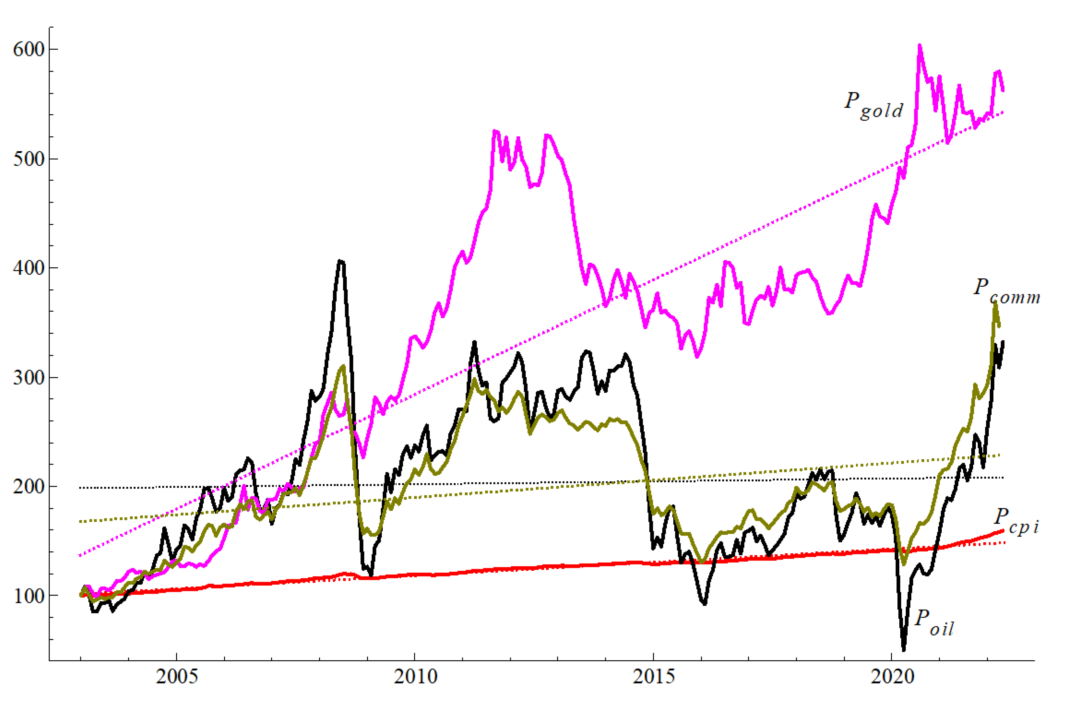
Figure 1 shows the level for nominal price of oil (Poil), along with three other price levels: the U.S. CPI (Pcpi); the price of non-monetary gold exports (Pgold); and the IMF’s Global Commodity Price Index (Pcomm); all of these price indexes are based on U.S. dollars and the figure shows them scaled to 100 for the first observation in January of 2003. (The data come from the St. Louis Federal Reserve’s Fred: https://fred.stlouisfed.org/ (accessed on 8 September 2022). Pcpi: Consumer Price Index for All Urban Consumers: All Items in U.S. City Average, Index 1982–1984 = 100, Monthly, Seasonally Adjusted. Fred mnemonic: CPIAUCSL. Poil: Crude Oil Prices: West Texas Intermediate (WTI)—Cushing, Oklahoma, USD per Barrel, Monthly, Not Seasonally Adjusted. Fred mnemonic: DCOILWTICO. Pgold: Export Price Index (End Use): Nonmonetary Gold, Index 2000 = 100, Monthly, Not Seasonally Adjusted. Fred mnemonic: IQ12260. Pcomm: Global Price Index of All Commodities, Index 2016 = 100, Monthly, Not Seasonally Adjusted: PALLFNFINDEXM.)
Inspection of the data reveals that these prices differ in their trend growth rate and their volatility. Thus, the choice of price index to deflate the price of oil has potential implications of interest for characterizing the relation between oil prices and exchange rates. The question I ask here is how sensitive the results of the existing literature to the choice of deflator for the price of oil are.
The first step in examining the implications of different price measures involves constructing the three alternative measures of the real price of oil:
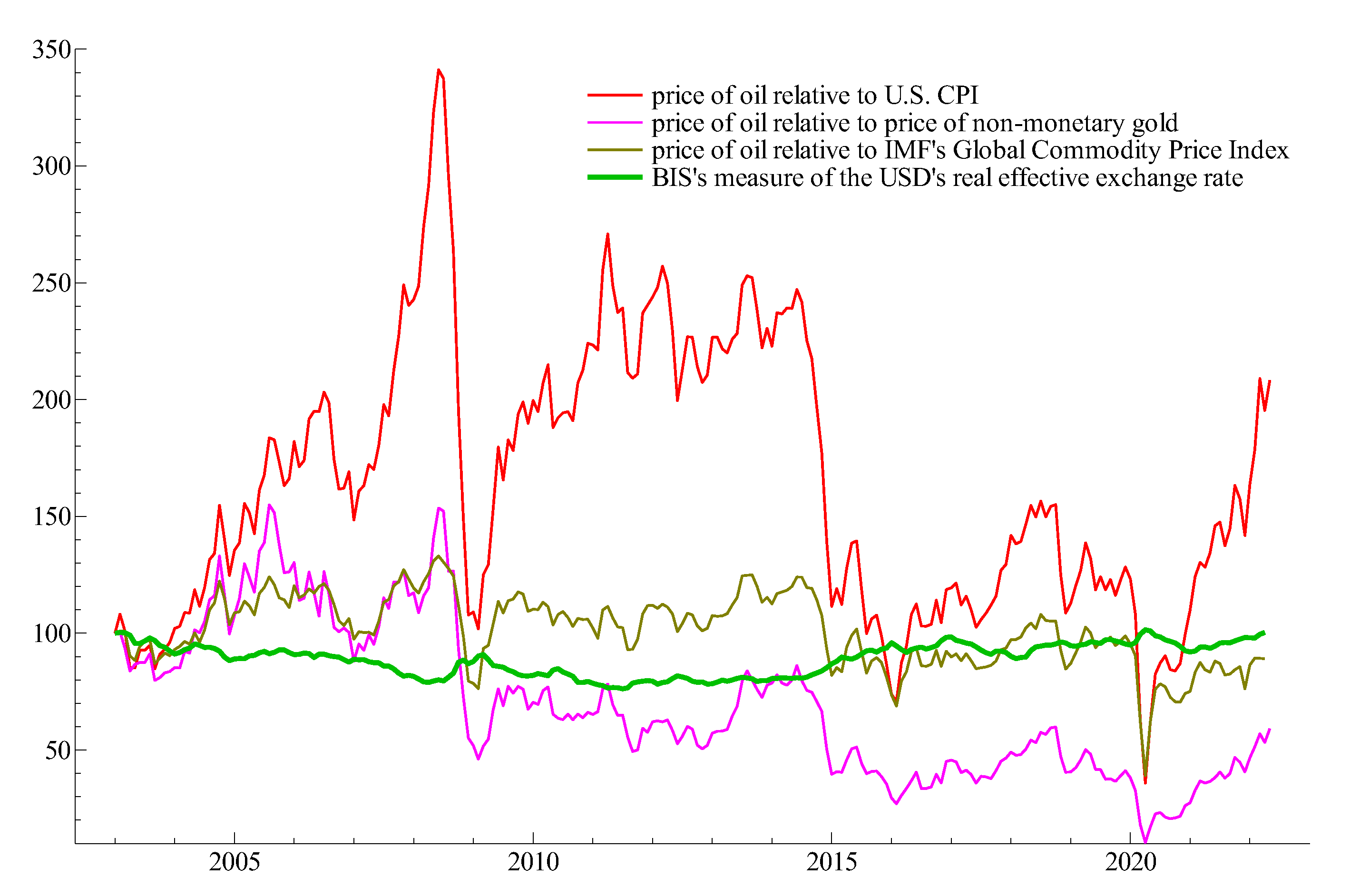
Figure 2 shows the time-series of these relative prices along with the BIS’ Real Effective Exchange Rate (Broad) for the U.S. dollar (The mnemonic in Fred is RBUSBIS). Inspection of the evidence reveals that the volatility of exceeds by far the volatility of and . Furthermore, the volatility of these last two relative prices is comparable to that of the effective real exchange rate. This empirical regularity plays a key role in interpreting the estimation results I report below.
3.2. Unconditional Correlations
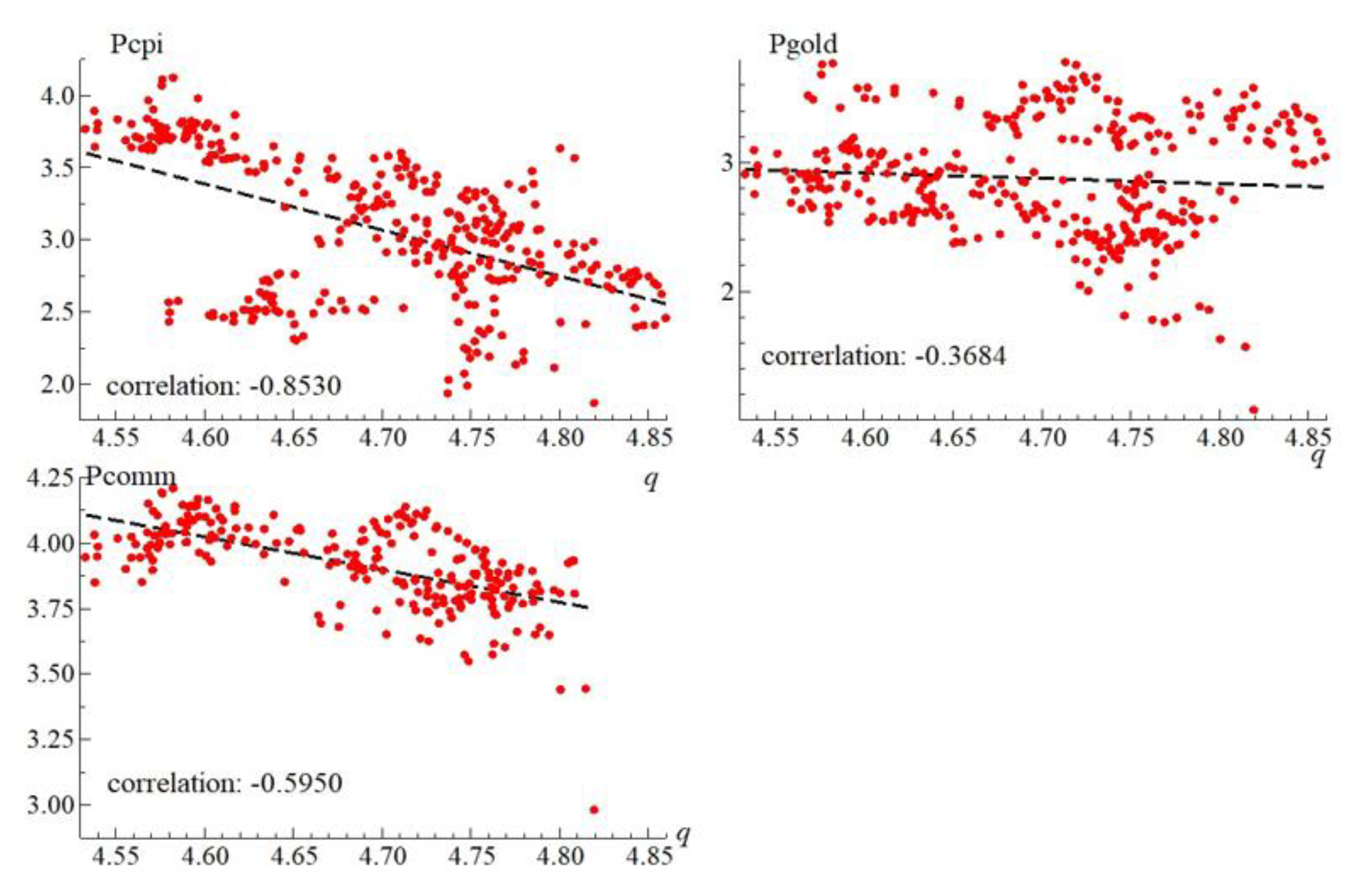
Figure 3 shows that one can make a case for an empirical relation between the logarithm of each measure of the real price of oil and the logarithm of the BIS measure of the real effective exchange rate of the U.S. dollar (q). The evidence reveals an inverse association between these two variables. However, the figures also reveal that the strength of this inverse association depends on what measure of relative prices is used.
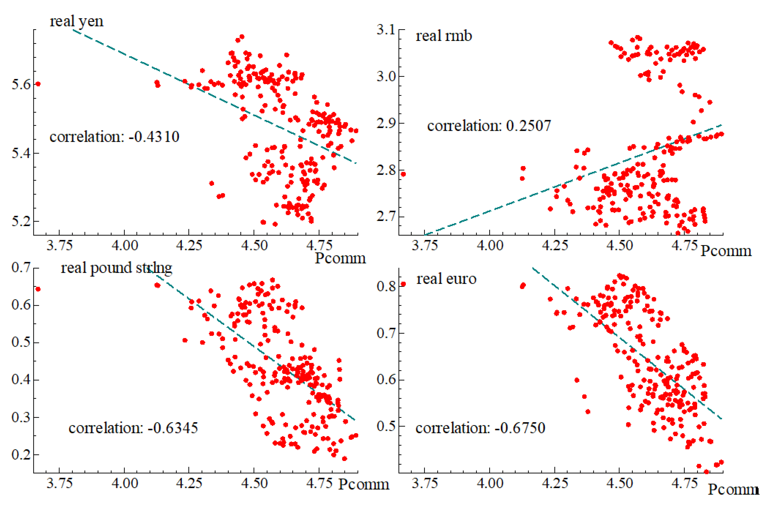
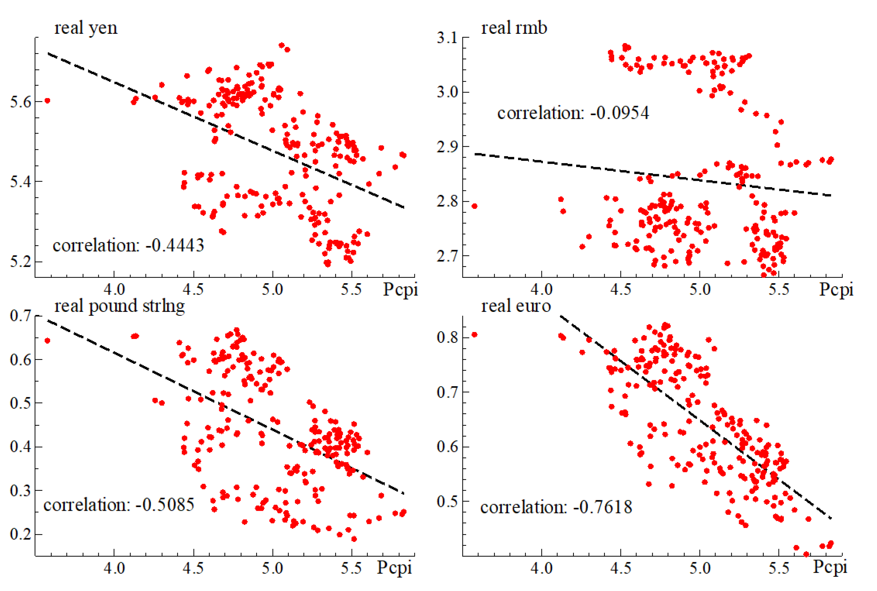
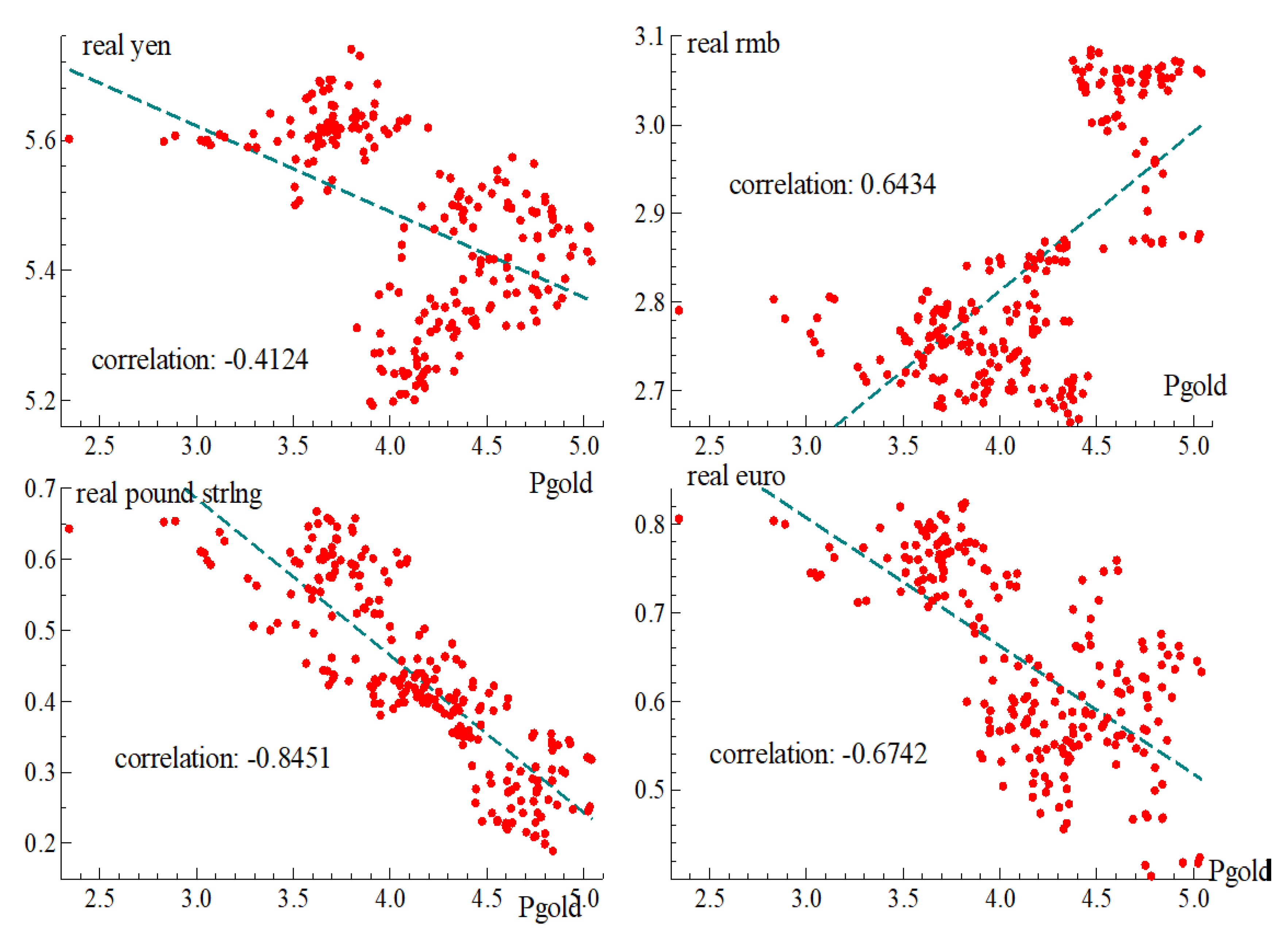
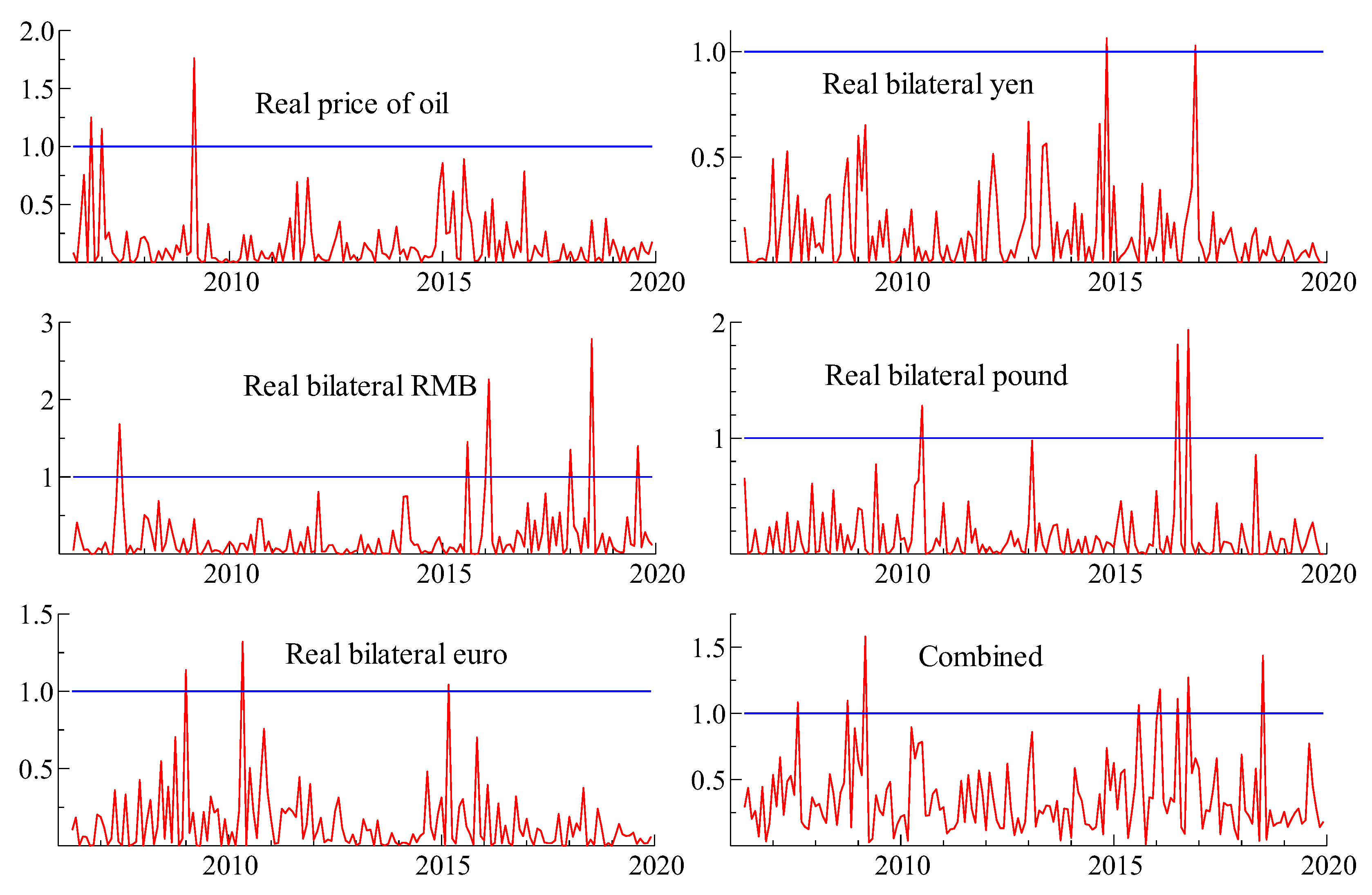
Figure 4, Figure 5 and Figure 6 show the relation between each measure of the real price of oil and four bilateral real exchange rates relative to USD using the currencies included in the IMF’s Special Drawing Rights (SDR): The U.S. dollar, the euro, the yen, the pound sterling, and the renminbi (more than 90 percent of international foreign exchange reserves are held in assets denominated in these currencies. See the IMF’s Currency Composition of Official Foreign Exchange Reserves. In terms of the global oil market, these five countries accounted for 55 percent of world oil consumption in 2019).
Overall, the figures make clear that measurement matters for characterizing the relation between the real price of oil and real exchange rates. What is not clear is which measure to use in applied work.
3.3. Vector Error Correction Modeling
To address this question, I use a Vector Error Correction Model, the parameters of which are estimated using the Johansen (1988) [1] cointegration technique as implemented by Doornik and Hendry (2003) [2]. This choice of modeling strategy is ideally suited for estimating short-run and long-run responses and for assessing the congruency of the model: white-noise residuals, parameter constancy, dynamic stability, and predictive accuracy.
For parameter estimation, I use a VAR of order 3 for the real price of oil and the real exchange rates for a total of six configurations: three models using the effective exchange rates and three models using the bilateral exchange rates. For estimation, I use monthly observations from January 2003 to December 2019 and reserve observations from January 2020 to April 2022 to examine the 1-step ex-post forecast performance for the price of oil for each configuration; Section 4 also reports the forecasts for the various measures of exchange rates. The paper’s forecast horizon includes the COVID-19 pandemic and the episode when the price of oil was negative for the first time.
The estimation results indicate that measurement matters for characterizing the cointegrating relation between oil prices and exchange rates (Table 3).
Using the CPI as the deflator, I replicate the literature’s empirical findings: an inverse and significant association between the CPI-adjusted oil price and real exchange rates, for both effective and bilateral measures of the real exchange rate. That inverse association is also present when using , but the point estimates are quite different from those based on . Specifically, estimates based on exhibit a nearly proportional relation between the real price of oil and the real exchange rates (effective and bilateral); using the , on the other hand, yields a more than proportional long-run relation between real oil prices and exchange rates.
Using the export price of gold as the deflator reveals that there is no long-run relation between the real price of oil and the effective exchange rate. If taken at face value, then this finding would imply that exchange rates do not affect the real price of oil. Yet, when I replace the effective exchange rate with the bilateral exchange rates, I find that they exert a significant effect on the real oil price with a virtually proportional relation. Note that the difference in coefficient estimates across models using are not due to differences in sample periods or estimation methods or econometric specifications: these design features are identical for the two models. Instead, the differences in estimates are due to the pitfalls of aggregation (Marquez and Merler 2020) [15].
Table 4 below reports the models’ predictive accuracy for the real price of oil; Section 4 reports the predictive accuracy for all the variables. This question is of interest because projections for oil prices and exchange rates play a role in the formulation of macroeconomic policy. (See the Minutes of the Federal Open Market Committee from May 2020 at https://www.federalreserve.gov/monetarypolicy/files/fomcminutes20200429.pdf (accessed on 8 September 2022). Further, the Federal Reserve Bank of New York’s Oil Price Dynamics Report [16] does not rely on effective exchange rates but on bilateral rates.) To this end, I focus now on the 1-step-ahead forecast record of the six configurations from January 2020 to April 2022, a period that includes the COVID-19 pandemic and the first time that the price of oil was negative. (As noted in the June 2020 Monetary Policy Report of the Federal Reserve, “On April 20, the price of front-month oil futures contracts for West Texas Intermediate (WTI) closed at negative $38 per barrel. These WTI futures contracts are settled by physical delivery; as worries about the lack of available storage space intensified, prices spiraled downward. Few contracts were actually traded at these negative prices, and prices recovered in the following days.” See https://www.federalreserve.gov/monetarypolicy/files/20200612_mprfullreport.pdf (accessed on 8 September 2022)). Inspection of the Root Mean Squared Forecast Errors (rsmfe) reveals that the predictive accuracy of models using either the CPI or the price of gold is lower than the predictive accuracy of the model based on the IMF Global Commodity Price Index (Table 4). The results also reveal that the RMSFE is largely invariant to the choice of exchange-rate measure.
Taken together, the results of Table 3 and Table 4 suggest that measurement matters for both estimation and forecasting. Note that I have yet to report the extent to which the data support the assumptions underlying the estimation results, which is what I do in the next section. Specifically, I examine the time-series properties of the variables, test for cointegration, for the direction of Granger causality, for parameter constancy, for white noise residuals, and for dynamic stability. However, to ease the expositional burden of these many details, Section 4 focuses on the reliability of the results using .
4. Materials and Methods
4.1. Formulation
I use a Vector Error Correction model treating both oil prices and exchange rates as endogenous (See Doornik, J. and D. Hendry (2013) [2]). This approach has two advantages: it addresses the spurious regression critique and differentiates between short- and long-run responses to shocks. Specifically,
where is a matrix of unknown coefficients; the specification includes seasonal dummies.
I assess the sensitivity of the results to the choice of exchange rates using the two models relying on the price of oil deflated by the IMF’s Global Commodity Price Index.
Model 1: BIS Effective Broad:
Model 2: Bilateral rates:
where
- is the logarithm of the real price of oil
- q is the logarithm of BIS’ broad real effective exchange rate of the dollar
- is the logarithm of the price-adjusted price of the dollar in terms of yen
- is the logarithm of the price-adjusted price of the dollar in terms of the pound sterling
- is the logarithm of the price-adjusted price of the dollar in terms of the renminbi
- is the logarithm of the price-adjusted price of the dollar in terms of the euro
Empirically, the existence of a long-run relation depends on the rank of . If the rank equals one, then and represents the long-run relation, with being the associated coefficients; characterizes responsiveness of to deviations from the long run.
4.2. Time-Series Properties
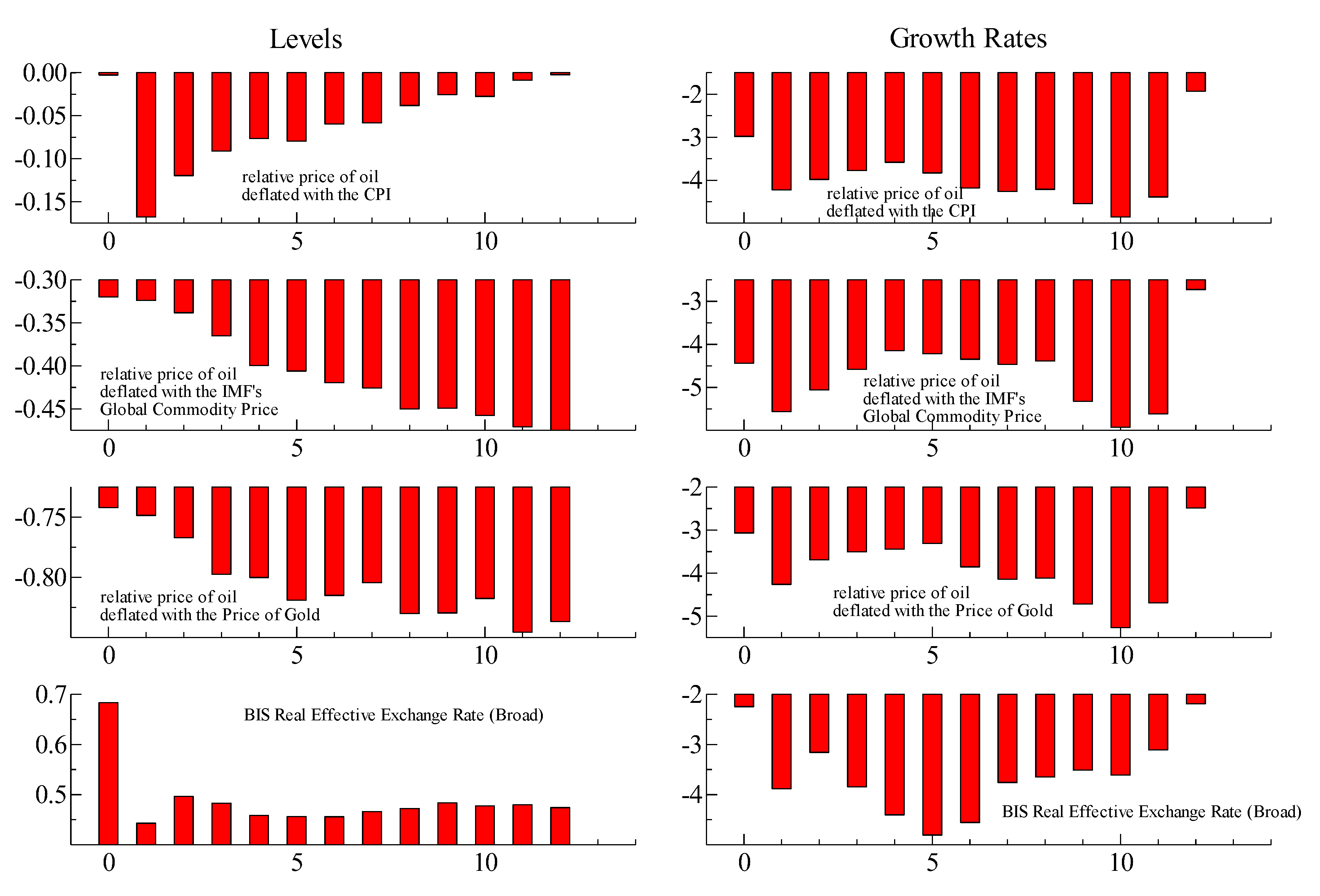
A necessary condition for the rank of being equal to one is for the variables to be integrated of order one. Testing this hypothesis involves testing the degree of stationarity for both the levels and the growth rates of the variables involved here. To that end, I use monthly observations from January 2003 to April 2022 and rely on Augmented Dickey Fuller tests with no intercept and with 12 lags. Figure 7 below shows the ADF-test statistics for the variables in log-levels in the left column and the growth rates in the right column.
The results show that one can reject the hypothesis that the log-levels of the variables are integrated of order zero and that one cannot reject the hypothesis that the growth rates are integrated of order zero. When combined, these two results imply that one cannot reject the hypothesis that the levels are integrated of order one.
4.3. Granger Causality
A property of interest is whether exchange rates Granger-cause the price of oil or the other way around. Testing the null hypothesis that exchange rates do not Granger-cause the price of oil involves excluding all of the exchange rates from the equation for the price of oil. Similarly, testing the null hypothesis that the price of oil does not Granger-cause exchange rates involves setting to zero the coefficients for oil prices in each of the four exchange rate equations. These two hypotheses are tested with a χ2(n) test where n is the number of restrictions.
According to the results, real exchange rates (effective or bilateral) Granger-cause the real price of oil but not the other way around (Table 5). In other words, excluding exchange rates from the equation for the price of oil carries a statistically significant loss of predictive power.
4.4. Cointegration
Having established that the series are integrated of order one, now I estimate the rank of using Johansen’s Trace and Max tests [1], corrected for degrees of freedom. Inspection of the results (Table 6) suggests that we cannot reject the hypothesis that the rank of is one. In other words, there is only one long-run relation among these variables.
4.5. Congruency
4.5.1. Parameter Constancy
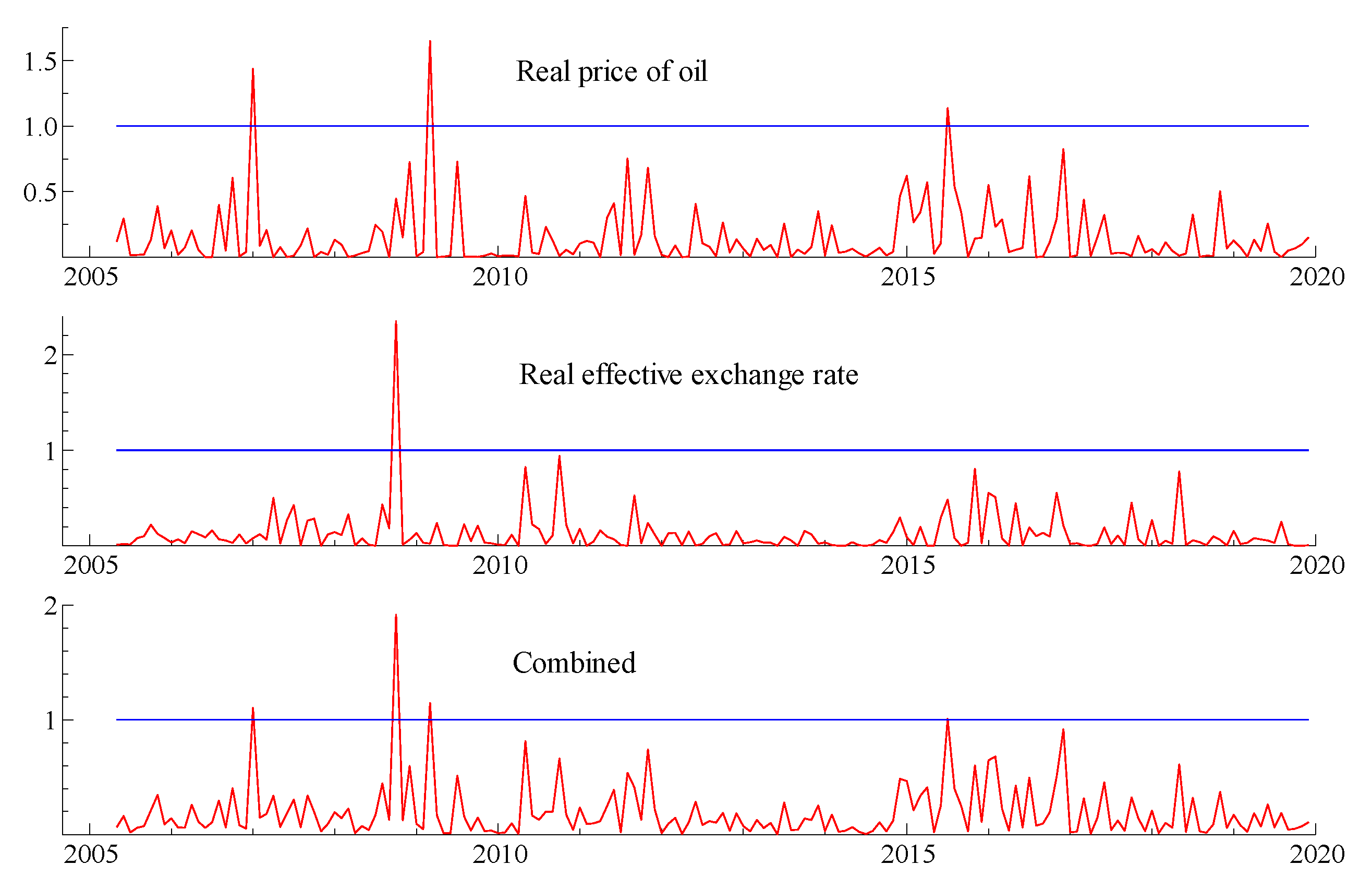
To test parameter constancy, I implement recursive least squares. This procedure begins with an initial sample to estimate the parameters and to generate one-period ahead test-statistics for prediction error. If the prediction error is statistically significant, then the parameters are not deemed constant for that initial sample. Then, the procedure augments the estimation sample by one observation, re-estimates the parameters, and re-generates another one-period-ahead prediction; if the prediction error is statistically significant, then the parameters are not deemed constant for the expanded sample. This process is repeated until all the observations are used.
The figures below show the normalized test statistic as a blue horizontal line and the prediction errors as the red line. If the red line is above the blue line, then prediction error is significant. I also test the joint hypothesis that both prediction errors are significant; the test results are labeled 1up-Chows. Figure 8 and Figure 9 show a handful of prediction errors that are significant, but most of the forecast errors are not significant. Based on these results, the models exhibit parameter constancy.
4.5.2. Residuals Properties
Table 7 reports the test results associated with the maintained assumptions used in estimation: serial independence, normality, and homoskedasticity. The results show that the residuals generally satisfy these assumptions but, to be sure, there are exceptions; this consideration needs to be considered when assessing the usefulness of the results.
4.5.3. Dynamic Stability
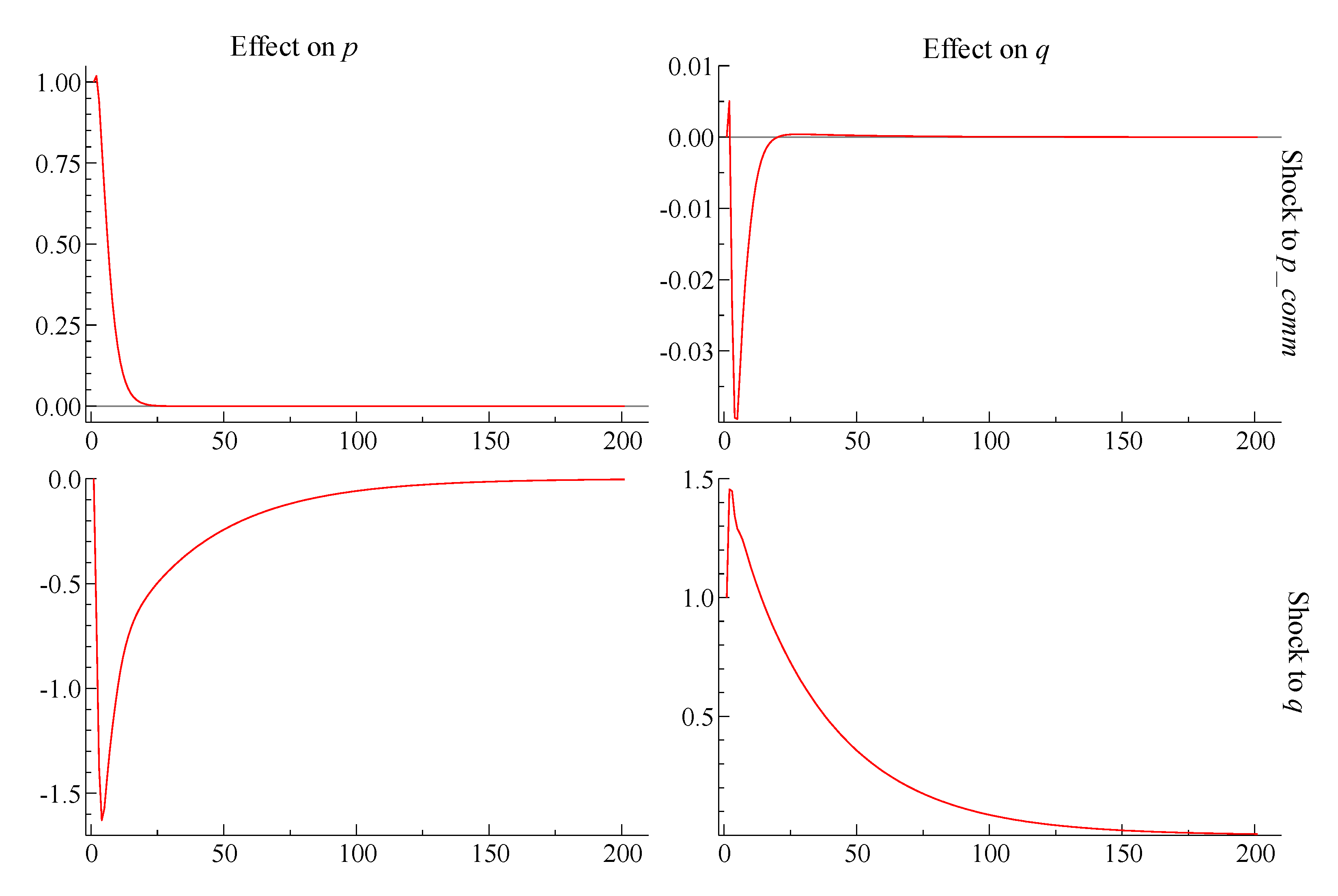
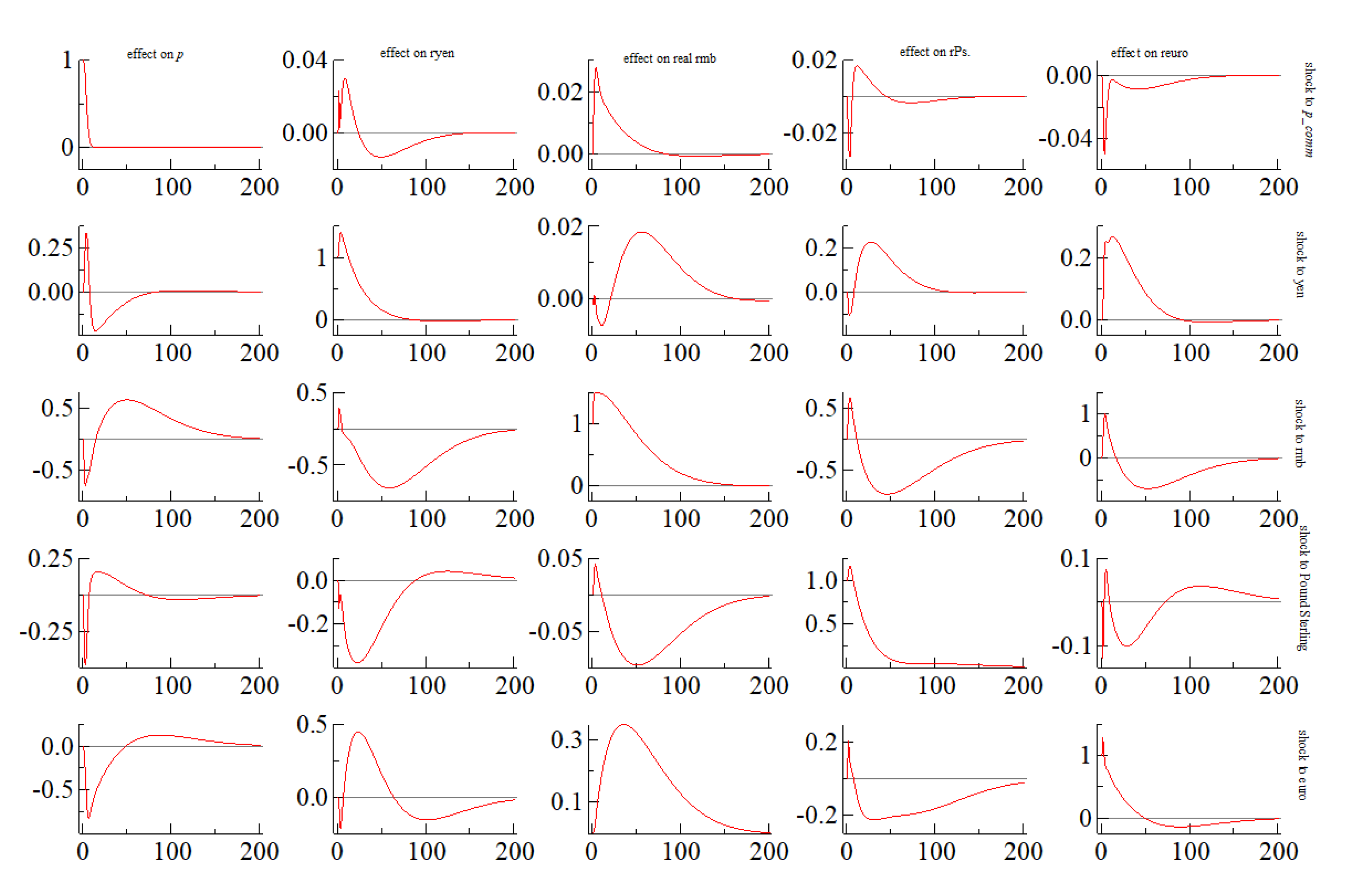
To examine whether the models are dynamically stable, I use impulse responses. These responses are implemented via a dynamic simulation that it is initiated at a value of zero and then shocked at a given date. The criterion for judging stability is that a temporary shock leads to temporary effects only. In other words, the impulse responses return to zero.
The results indicate two properties of interest (Figure 10 and Figure 11). First, the models are dynamically stable. Second, for the model using the effective exchange rate, a unitary shock to the residual of the exchange rate lowers the price of oil; for the model using bilateral exchange rates, a shock to the residuals of these equations also lowers the price of oil initially.
4.5.4. Forecasting Performance
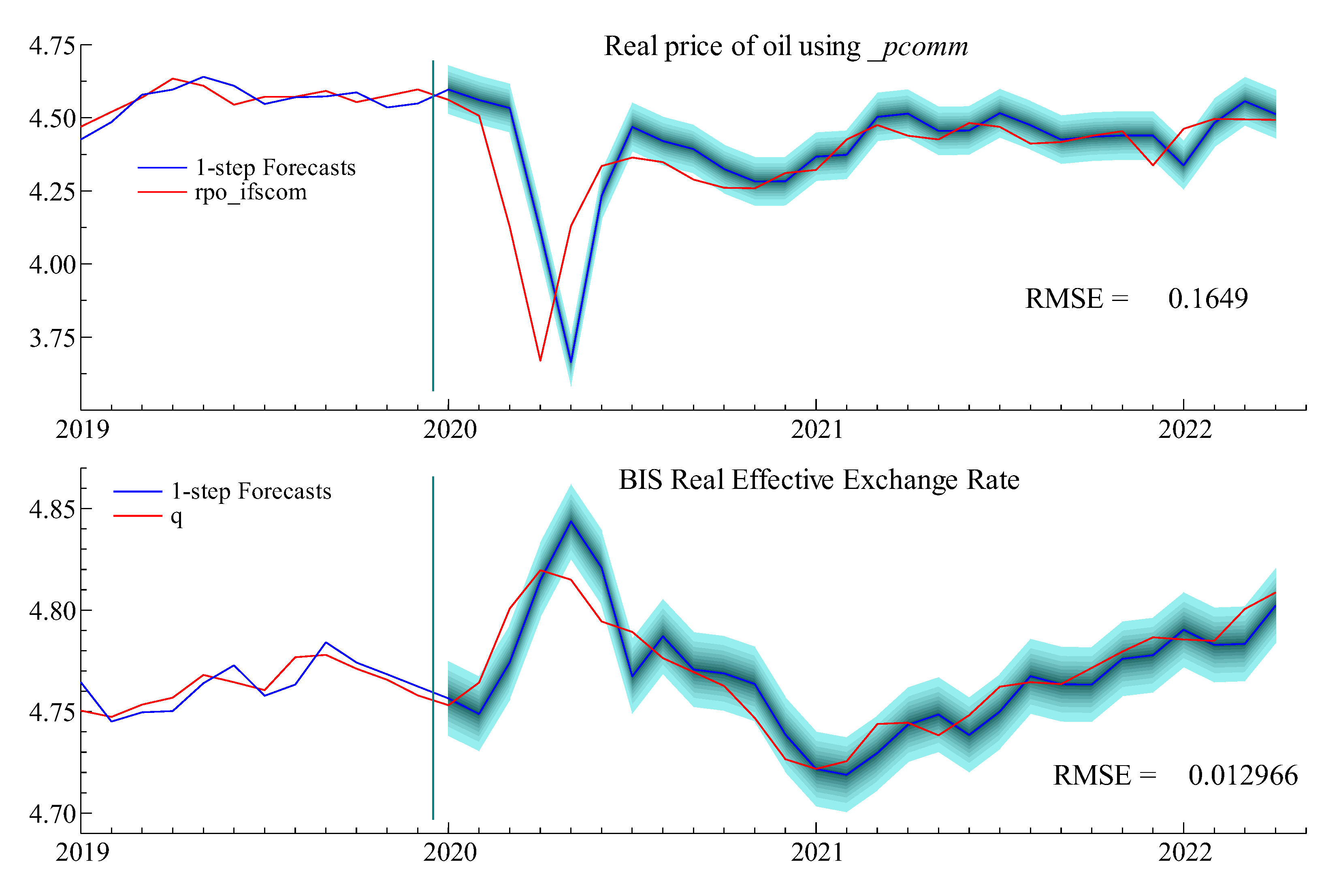
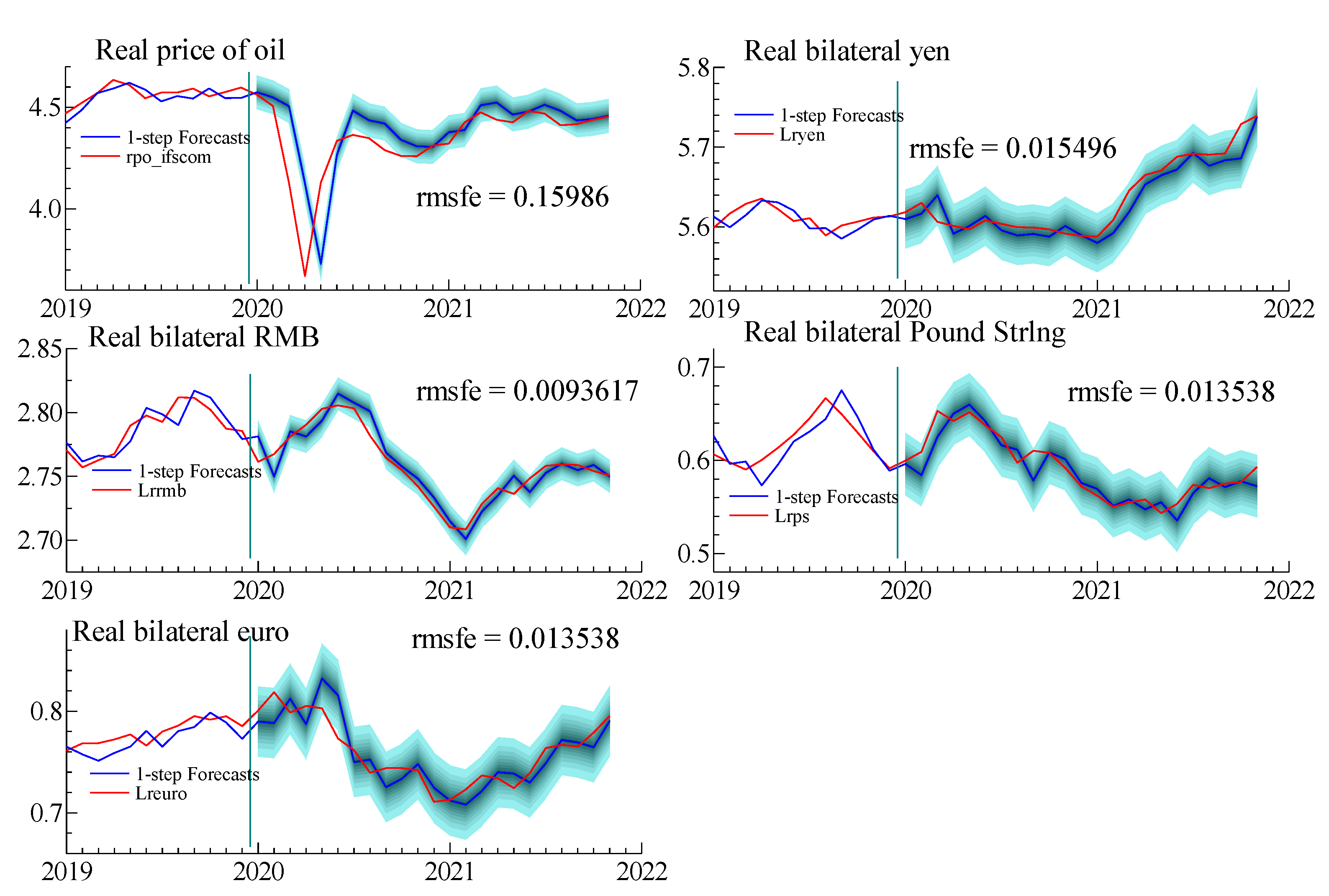
Figure 12 and Figure 13 show the 95 percent confidence bands of the one-step-ahead forecasts from models using pcomm from January 2020 to April 2022 (the “one-step-ahead” refers to the practice of financial forecasters of starting their forecasts from the most recent data).
Inspection of the results reveal a large forecast error for the real price of oil in March of 2020, which is the start of the global COVID-19 pandemic. Predictions afterwards, however, are contained within the 95 percent confidence bands, suggesting that the forecast errors are not statistically significant; forecasts for the exchange rates are generally well within their 95 percent confidence bands. This finding suggests that large error for the real price of oil in March 2020 is not likely to be the result of forecast errors in the exchange rates spilling over to the forecast for the price of oil.
5. Conclusions
The main conclusion of this paper is that, using a Vector Error Correction model, the relation between real oil prices and real exchange rates is not invariant to the choice of deflator for the price of oil. Further, using the IMF’s Global Commodity Price Index points to a long-run relation with a unitary slope between real oil prices and real value of the dollar. Finally, this choice of deflator has the lowest forecast errors.
To be sure, I have not examined whether these findings are robust to changes in methodologies or to a longer list of candidate deflators for the price of oil. Similarly, I have not examined whether the models used here can explain the forecasts from other models (forecast encompassing). Furthermore, though the congruency test results do not reject most of the assumptions used for parameter estimation, these results do not imply accepting the model used here.
In the end, much work remains to be completed along the lines of measurement, estimation methods, and congruency tests. Extending the results of this paper will, however, emphasize its main point—namely, that measurement matters.
Funding
This research received no external funding.
Institutional Review Board Statement
Not Applicable.
Informed Consent Statement
Not Applicable.
Data Availability Statement
Apart from data transformations (e.g., logs, changes, and ratios) all the data come from https://fred.stlouisfed.org/ (accessed on 8 September 2022).
Acknowledgments
I want to acknowledge the truly helpful comments and criticisms from three anonymous referees. I also want to acknowledge the research assistance of Hanting Wu. All the calculations in this paper were carried out using PcGive 8.03; see Doornik, J. and D. Hendry 2013.
Conflicts of Interest
The author declares no conflict of interest.
References
- Johansen, S. Statistical Analysis of Cointegration Vectors. J. Econ. Dyn. Control. 1988, 12, 231–254. [Google Scholar] [CrossRef]
- Doornik, J.; Hendry, D. Empirical Econometric Modeling Vols. I and II.; Timberlake Consultants: London, UK, 2013. [Google Scholar]
- Krugman, P.R. Oil and the Dollar; NBER Working Paper: Cambridge, MA, USA, 1980. [Google Scholar]
- Breitenfellner, A.; Cuaresma, J.C. Crude Oil Prices and the USD/EUR Exchange Rate. Monet. Policy Econ. 2008, 4. [Google Scholar]
- Benassy-Quere, A.; Mignon, V.; Penot, A. China and the Relationship between the Oil Price and the Dollar. CEPII Working Paper. Energy Policy 2005, 35, 5795–5805. [Google Scholar] [CrossRef]
- Cheng, K.C. Dollar Depreciation and Commodity Prices. World Economic Outlook; IMF: Washington, DC, USA, 2008. [Google Scholar]
- Huang, B.; Lee, C.; Chang, Y.; Lee, C. Dynamic linkage between oil prices and exchange rates: New global evidence. Empir. Econ. 2020, 61, 719–742. [Google Scholar] [CrossRef]
- Beckmann, J.; Czudaj, R.; Arora, V. The Relationship between Oil Prices and Exchange Rates: Theory and Evidence. EIA Work. Pap. Ser. 2017, 1–62. [Google Scholar] [CrossRef]
- Golub, S.S. Oil Prices and Exchange Rates. Econ. J. 1983, 93, 576–593. [Google Scholar] [CrossRef]
- Amano, R.A.; Norden, S. Oil Prices and the Rise and Fall of the US Real Exchange Rate. J. Int. Money Financ. 1998, 17, 299–316. [Google Scholar] [CrossRef]
- Reboredo, J.C.; Rivera-Castro, M.; Zebende, G. Oil and US dollar exchange-rate dependence: A detrended cross-correlation approach. Energy Econ. 2014, 42, 132–139. [Google Scholar] [CrossRef]
- Fratzscher, M.; Schneider, D.; van Robays, I. Oil Prices, Exchange Rates and Asset Prices; ECB Working Paper: Frankfurt, Germany, 2014; p. 1689. [Google Scholar]
- Grisse, C. What Drives the Oil-Dollar Correlation? Federal Reserve Bank of New York: New York, NY, USA, 2010. [Google Scholar]
- Yousefi, A.; Wirjanto, T.S. A Stylized Exchange Rate Pass-through Model of Crude Oil Price Formation. OPEC Rev. 2005, 29, 177–187. [Google Scholar] [CrossRef]
- Marquez, J.; Merler, S. A Note on the Empirical Relation between Oil Prices and the Value of the Dollar. J. Risk Financ. Manag. 2020, 13, 164. [Google Scholar] [CrossRef]
- Federal Reserve Bank of New York. Oil Price Dynamics Report. 2020. Available online: https://www.newyorkfed.org/research/policy/oil_price_dynamics_report.html (accessed on 8 September 2022).
Figure 1.
Price Levels for selected groupings.

Figure 2.
Relative Prices.

Figure 3.
Real Oil Prices and Real Effective Exchange Rate—Sensitivity to the Oil-price Deflator.

Figure 4.
Real Bilateral Exchange Rates and .

Figure 5.
Real Bilateral Exchange Rates and .

Figure 6.
Real Bilateral Exchange Rates and .

Figure 7.
ADF tests for levels (left panel) and growth rates (right panel). The critical values for rejection are: 5% = −1.94, 1% = −2.58.
Figure 7.
ADF tests for levels (left panel) and growth rates (right panel). The critical values for rejection are: 5% = −1.94, 1% = −2.58.

Figure 8.
Constancy Tests for model using and Effective Exchange Rates. Blue line denotes the 1% critical rejection value.
Figure 8.
Constancy Tests for model using and Effective Exchange Rates. Blue line denotes the 1% critical rejection value.

Figure 9.
Parameter Constancy Tests for model using and Bilateral Exchange Rates. Blue line denotes the 1% critical rejection value.
Figure 9.
Parameter Constancy Tests for model using and Bilateral Exchange Rates. Blue line denotes the 1% critical rejection value.

Figure 10.
Responses for and Effective Exchange Rate. Note: row-headings list the residual that is being shocked; the column-headings indicate the variable that is affected.
Figure 10.
Responses for and Effective Exchange Rate. Note: row-headings list the residual that is being shocked; the column-headings indicate the variable that is affected.

Figure 11.
Responses for Bilateral Exchange Rates. Note: row-headings list the residual that is being shocked; the column-headings indicate the variable that is affected.
Figure 11.
Responses for Bilateral Exchange Rates. Note: row-headings list the residual that is being shocked; the column-headings indicate the variable that is affected.

Figure 12.
One-step-ahead forecast errors for model using effective exchange rates.

Figure 13.
One-step-ahead forecast errors for model using bilateral exchange rates.


Table 1.
Design Characteristics of Selected Studies (by publication date).
| Study | Measure of USD | Sample | Estimation | China |
|---|---|---|---|---|
| Method | Included? | |||
| Huang et al. (2020) 7] | Bilateral Rates | 1997–2015—Monthly | PMG | yes |
| Reboredo et al. (2014) [11] | Bilateral Rates | 2000–2012—Monthly | Cross-Corr. | no |
| Fratzscher et al. (2014) [12] | NEER | 2001–2012—Daily | Het. Ident. | no |
| Grisse (2010) [13] | NEER | 2003–2010—Weekly | SVAR | no |
| Breitenfellner et al. (2008) [4] | (EUR/USD) | 1983–2006—Monthly | VECM | no |
| Cheng (2008) [6] | NEER & REER | 2000–2007—Monthly | DOLS | no |
| Yousefi et al. (2005) [14] | REER | 1989–1999—Monthly | Egl–Grger | no |
| Bénassy-Quéré et al. (2005) [5] | REER & (EUR/USD) | 1974–2004—Monthly | ECM | yes |
| Amano et al. (1998) [10] | REER | 1972–1993—Monthly | VECM | no |
| This study | REER & Bilateral Rates | 2003–2022—Monthly | VECM | yes |
Memo SVAR: Structural VAR; VECM: Vector Error Correction; DOLS: Dynamic OLS; PMG: pooled mean group, Het. Ident: identification via Heteroskedasticity; Egl–Grger: Engle–Granger cointegration; REER: real effective exchange rate; NEER: nominal effective exchange rate; EUR/USD is the bilateral exchange rate between the Euro and the U.S. dollar.
Table 2.
Reported Statistical Tests of Selected Studies (by publication date).
| Parameter | Residuals’ | ||||
|---|---|---|---|---|---|
| Study | Constancy | Properties | Forecasts | Stationarity | Causality |
| Huang et al. (2020) [7] | no | no | no | yes | no |
| Reboredo et al. (2014) [11] | no | no | no | no | yes |
| Fratzscher et al. (2014) [12] | no | no | no | no | yes |
| Grisse (2010) [13] | no | no | no | no | yes |
| Breitenfellner et al. (2008) [4] | no | no | yes | no | no |
| Cheng (2008) [6] | no | no | no | no | no |
| Yousefi et al. (2005) [14] | no | no | no | no | no |
| Bénassy-Quéré et al. (2005) [5] | no | indep. | no | yes | yes |
| Amano et al. (1998) [10] | no | no | yes | yes | yes |
| This study | yes | yes | yes | yes | yes |
Table 3.
Long-run effect of a 1% appreciation in the real value of the dollar on the real price of oil—2003–2019.
Table 3.
Long-run effect of a 1% appreciation in the real value of the dollar on the real price of oil—2003–2019.
| Measure of Deflator for Nominal Price of Oil | |||||||
|---|---|---|---|---|---|---|---|
| Pcpi | Pcom | Pgold | |||||
| Measure of Exchange Rate | coeff | se | coeff | se | coeff | se | |
| Effective | −3.85 | 0.56 | −0.84 | 0.31 | −3.21 | 2.42 | |
| Bilateral | Lryen | 0.44 | 0.42 | 0.37 | 0.15 | 0.897 | 0.315 |
| Lrrmb | −0.60 | 0.43 | 0.15 | 0.15 | 1.759 | 0.318 | |
| Lrps | 0.72 | 0.66 | 0.23 | 0.23 | −0.383 | 0.488 | |
| Lreuro | −3.88 | 0.83 | −1.47 | 0.29 | −3.244 | 0.616 | |
| Sum | −3.31 | 0.81 | −0.72 | 0.27 | −0.971 | 0.55 | |
Table 4.
Root Mean Squared Forecast Error (rmfse): January 2020–April 2022.
| Measure of Deflator | |||
|---|---|---|---|
| Pcpi | Pcomm | Pgold | |
| Measure of Exchange Rate | |||
| Effective | 21.717% | 16.490% | 22.261% |
| Bilateral | 21.748% | 15.986% | 22.029% |
Table 5.
Granger Causality Tests: 2003:1–2022:4.
| H0 | n | p-Value for χ²(n) | |
|---|---|---|---|
| Model 1 | pq | 3 | 0.296 |
| qp | 3 | 0.017 | |
| Model 2 | pr | 12 | 0.93 |
| rp | 12 | 0.036 |
p: real price of oil; q: of model 1; r: 4 × 1 vector of bilateral real exchange rates of model 2.
Table 6.
p-values for Johansen’s Rank Tests 2003:1–2019:12.
| Model 1 | Model 2 | |||
|---|---|---|---|---|
| Rank of Π | Max | Trace | Max | |
| 0 | 0.004 | 0.008 | 0.007 | 0 |
| 1 | 0.068 | 0.068 | 0.599 | 0.663 |
| 2 | 0.696 | 0.776 | ||
| 3 | 0.664 | 0.872 | ||
| 4 | 0.327 | 0.327 |
Indep.: test of autocorrelation of residuals; F-test to an AR(7) of estimated residuals. Homosk.: test of homoskesdasticity of residuals; F-test to an AR(7) of estimated squared residuals. Normality: test of normality; χ2(2).
Table 7.
p-values for statistical properties of residuals 2003:1–2019:12.
| H0: Indep. | H0: Homosk. | H0: Normality | ||
|---|---|---|---|---|
| Model 1 | pcomm | 0.1297 | 0.129 | 0.3362 |
| q | 0.2876 | 0.9537 | 0.0001 | |
| Model 2 | pcomm | 0.385 | 0.669 | 0.117 |
| ryen/$ | 0.219 | 0.2421 | 0.8608 | |
| reuro/$ | 0.316 | 0.0002 | 0.9368 | |
| rpound/$ | 0.311 | 0.0182 | 0.0295 | |
| rrmb/$ | 0.749 | 0.3127 | 0.0002 |
Indep.: test of autocorrelation of residuals; F-test to an AR(7) of estimated residuals. Homosk.: test of homoskesdasticity of residuals; F-test to an AR(7) of estimated squared residuals. Normality: test of normality; χ2(2).
Publisher’s Note: MDPI stays neutral with regard to jurisdictional claims in published maps and institutional affiliations. |
© 2022 by the author. Licensee MDPI, Basel, Switzerland. This article is an open access article distributed under the terms and conditions of the Creative Commons Attribution (CC BY) license (https://creativecommons.org/licenses/by/4.0/).
Share and Cite
MDPI and ACS Style
Marquez, J. Oil Prices and Exchange Rates: Measurement Matters. Commodities 2022, 1, 50-64. https://doi.org/10.3390/commodities1010005
AMA Style
Marquez J. Oil Prices and Exchange Rates: Measurement Matters. Commodities. 2022; 1(1):50-64. https://doi.org/10.3390/commodities1010005
Chicago/Turabian StyleMarquez, Jaime. 2022. "Oil Prices and Exchange Rates: Measurement Matters" Commodities 1, no. 1: 50-64. https://doi.org/10.3390/commodities1010005