
Generalized Unit Half-Logistic Geometric Distribution: Properties and Regression with Applications to Insurance
 ,
, 
 and
and
Abstract
:1. Introduction
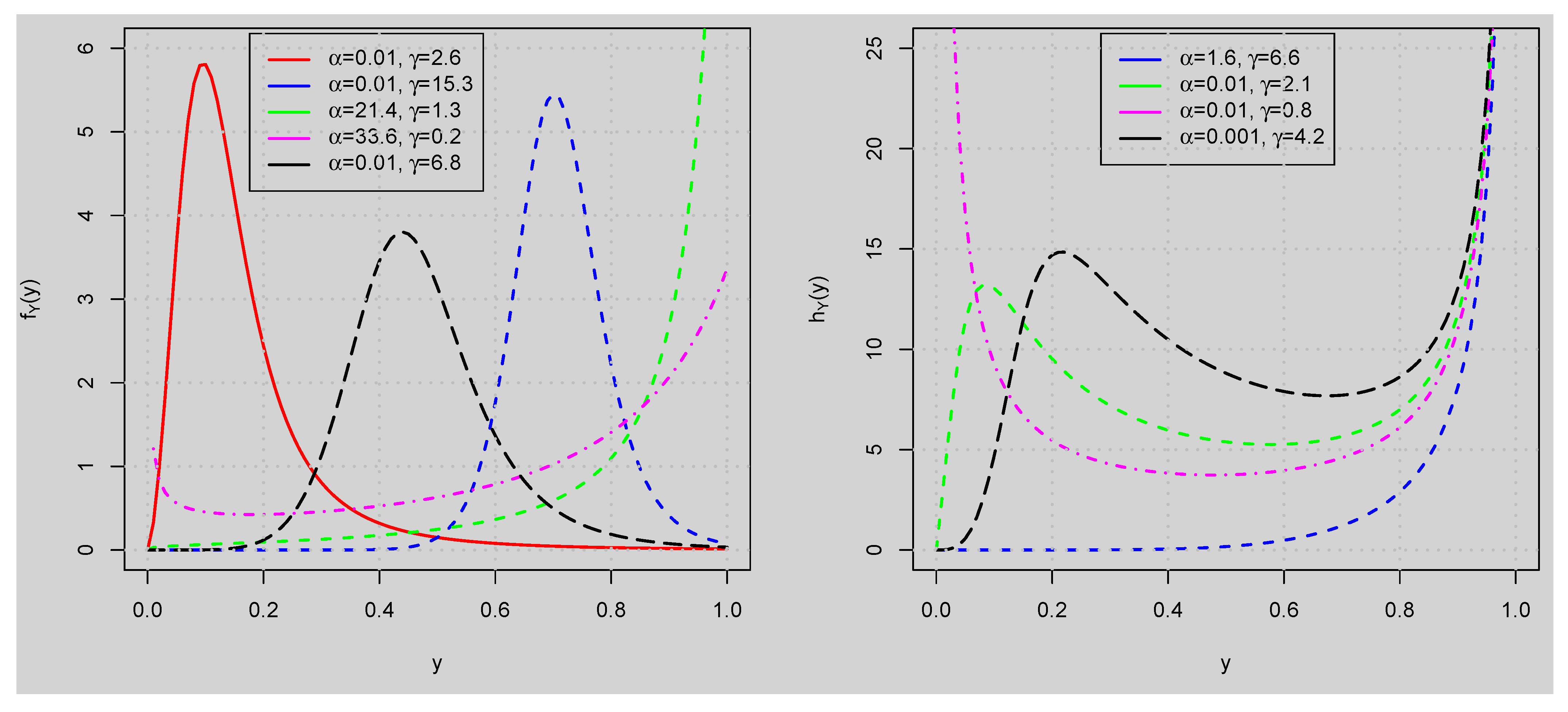
2. GUHLG Distribution
3. Some Statistical Properties
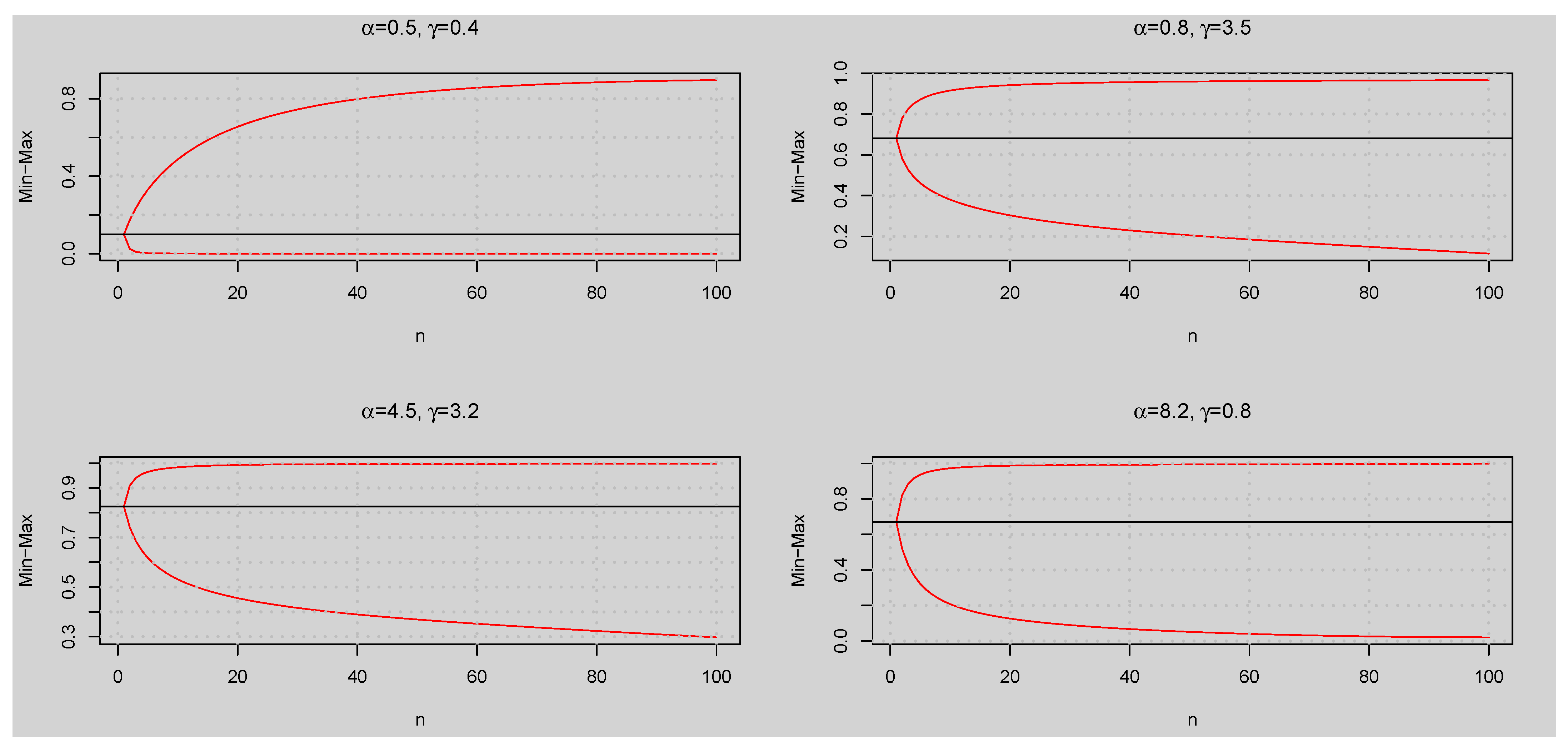
3.1. Distributional Inequalities
3.2. Quantile Function
- Set the values of the parameters and .
- Obtain p as a random observation of a random variable that follows the standard uniform distribution, .
- Estimate .
- Repeat steps 2 and 3 n times to obtain n values: .
3.3. Moments
3.4. Order Statistics
4. Parameter Estimation
Simulation Studies
- Generate 5000 random samples of size and 1000 from the GUHLG distribution using the algorithm discussed in Section 3.3.
- Find the ML estimates of the parameters.
- Compute the MEs, ABs, ARBs, RMSEs, and CPs of the parameters.
- Repeat steps 1 to 3 for the three parameter combinations.
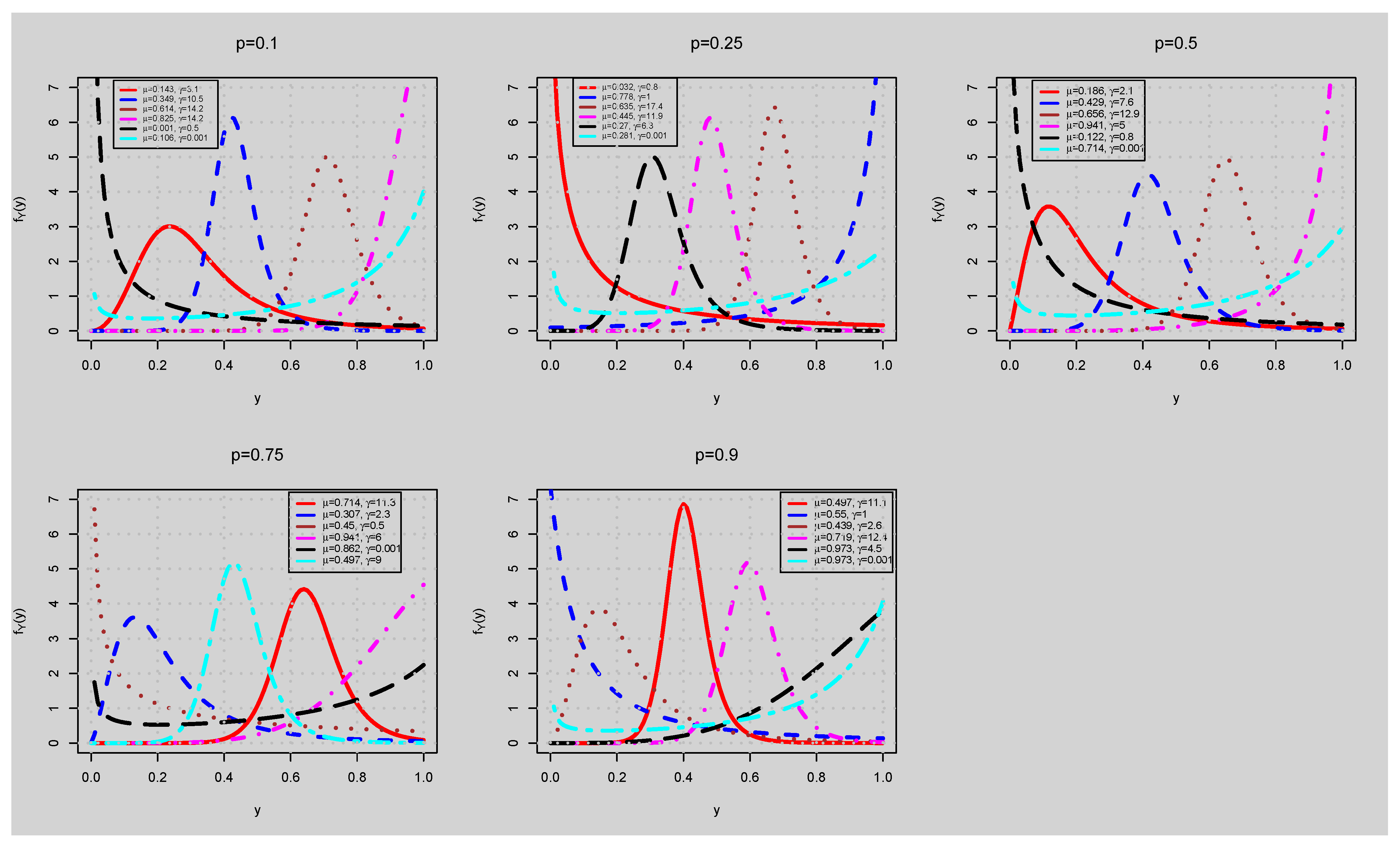
5. Quantile Regression
5.1. Residual Analysis
5.2. Monte Carlo Simulations for Regressions
- Generate the exogenous variables and from the Bernoulli and standard normal distributions, respectively.
- Generate the endogenous variable usingwhere is an observation from standard uniform distribution, and .
- Compute the ML estimates of the parameters of the regression model.
- Compute the MEs, ABs, ARB, RMSEs and CPs of the parameters.
- Repeat steps 1 to 4 for the two parameter combinations.
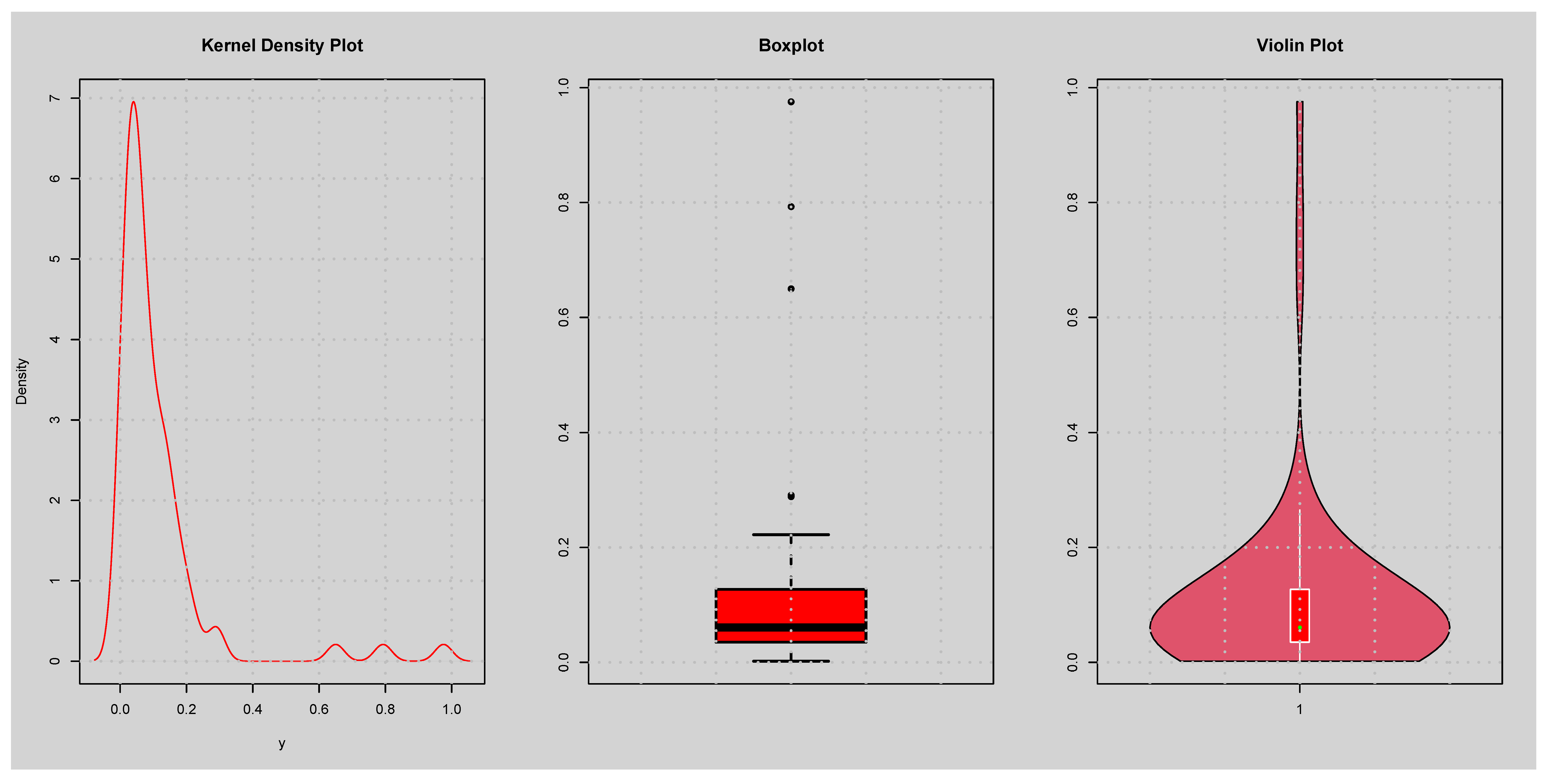
6. Application
6.1. Univariate Application
6.2. Multivariate Application
6.2.1. Frequentist Approach
- ASSUME: Ratio of per occurrence retention levels to total assets.
- CAP: The firm’s use of captive (1 if yes and 0 if no).
- SIZELOG: Logarithm of the firm’s total asset value.
- INDCOST: Industry average of premiums plus uninsured losses divided by total assets (a measure of the firm’s industry risk).
- CENTRAL: Importance of local managers in choosing local retention levels.
- SOPH: Importance of analytical tools in making risk management decisions.
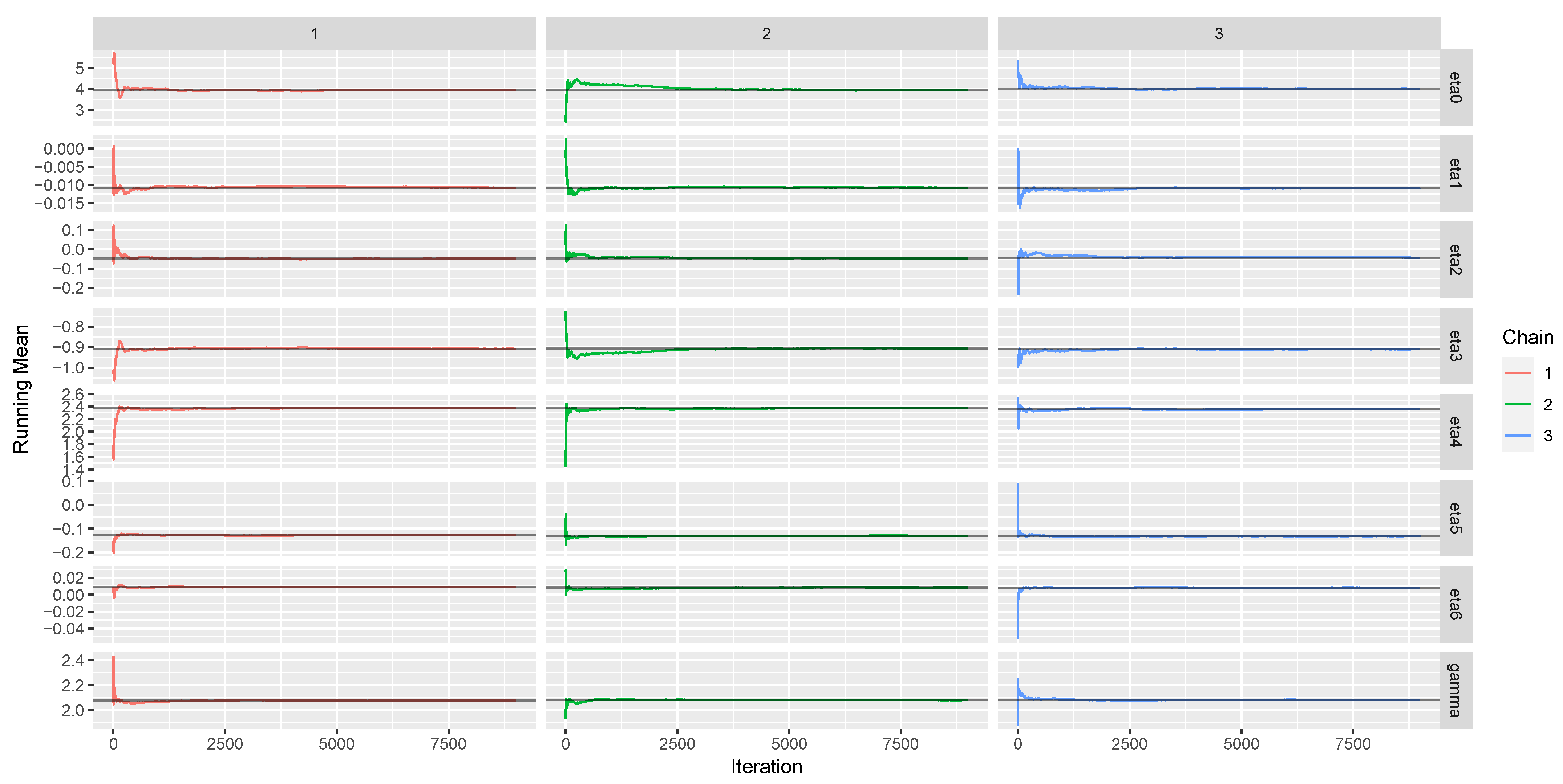
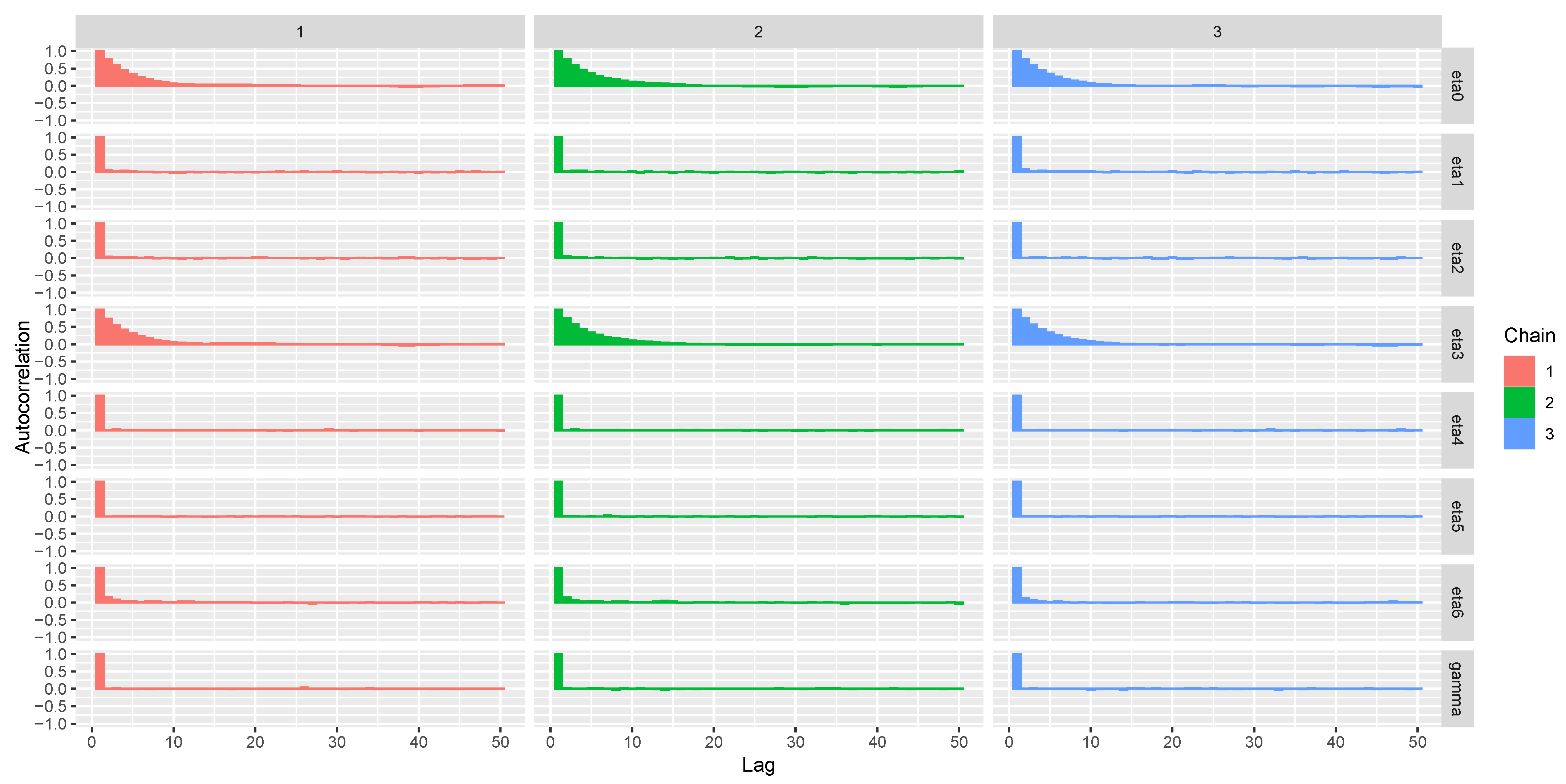
6.2.2. Bayesian Approach
7. Conclusions
Author Contributions
Funding
Institutional Review Board Statement
Informed Consent Statement
Data Availability Statement
Acknowledgments
Conflicts of Interest
References
- Ramadan, A.T.; Tolba, A.H.; El-Desouky, B.S. A unit half-logistic geometric distribution and its application in insurance. Axioms 2022, 11, 676. [Google Scholar] [CrossRef]
- Abubakari, A.G.; Luguterah, A.; Nasiru, S. Unit exponentiated Fréchet distribution: Actuarial measures, quantile regression and applications. J. Indian Soc. Probab. Stat. 2022, 23, 387–424. [Google Scholar] [CrossRef]
- Alanzi, A.R.A.; Rafique, M.Q.; Tahir, M.H.; Sami, W.; Jamal, F. New modified Kumaraswamy distribution: Actuarial measures and applications. J. Math. 2022, 1–18. [Google Scholar] [CrossRef]
- Ahmad, Z.; Mahmoudi, E.; Alizadeh, M. Modelling insurance losses using a new beta power transformed family of distributions. Commun.-Stat.-Simul. Comput. 2022, 51, 4470–4491. [Google Scholar] [CrossRef]
- Mazucheli, J.; Menezes, A.F.; Ghitany, M.E. The unit Weibull distribution and associated inference. J. Appl. Probab. Stat. 2018, 13, 1–22. [Google Scholar]
- Ahmad, Z.; Mahmoudi, E.; Dey, S.; Khosa, S.K. Modeling vehicle insurance loss data using a new member of the T-X family of distributions. J. Stat. Theory Appl. 2020, 19, 133–147. [Google Scholar] [CrossRef]
- Jodrá, P.; Jiménez-Gamero, M.D. A quantile regression for bounded responses based on exponential geometric distribution. Revstat 2020, 18, 415–436. [Google Scholar]
- Ahmad, Z.; Mahmoudi, E.; Hamedani, G.G. A family of loss distributions with an application to the vehicle insurance loss data. Pak. J. Stat. Oper. Res. 2019, 15, 731–744. [Google Scholar] [CrossRef]
- Mazucheli, J.; Menezes, A.F.; Dey, S. Unit-Gompertz distribution with applications. Statistica 2019, 79, 25–43. [Google Scholar]
- Gómez-Déniz, E.; Sordo, M.A.; Calderín-Ojeda, E. The log-Lindley distribution as an alternative to the beta regression model with applications in insurance. Insur. Math. Econ. 2014, 54, 49–57. [Google Scholar] [CrossRef]
- Al-Mofleh, H.; Afify, A.Z.; Ibrahim, N.A. A new extended two-parameter distribution: Properties, estimation methods and, applications in medicine and geology. Mathematics 2020, 8, 1578. [Google Scholar] [CrossRef]
- Jodrá, P.; Gómez, H.W.; Jiménez-Gamero, M.D.; Alba-Fernández, M.V. The power Muth distribution. Math. Model. Anal. 2017, 22, 186–201. [Google Scholar] [CrossRef]
- Iqbal, Z.; Tahir, M.M.; Riaz, N.; Ali, S.A.; Ahmad, M. Generalized inverted Kumaraswamy distribution: Properties and application. Open J. Stat. 2017, 7, 645–662. [Google Scholar] [CrossRef]
- Iqbal, Z.; Hasnain, S.A.; Salman, M.; Ahmad, M.; Hamedani, G.G. Generalized exponentiated moment exponential distribution. Pak. J. Stat. 2014, 30, 537–554. [Google Scholar]
- Cordeiro, G.M.; Brito, R.S. The beta power distribution. Braz. J. Probab. Stat. 2012, 26, 88–112. [Google Scholar]
- Jose, K.K.; Joseph, A.; Ristic, M.M. A Marshall-Olkin beta distribution and its applications. J. Probab. Stat. Sci. 2009, 7, 173–186. [Google Scholar]
- Shaked, M.; Shanthikumar, J.G. Stochastic Orders; Wiley: New York, NY, USA, 2007. [Google Scholar]
- Mazzoccoli, A.; Naldi, M. The expected utility insurance premium principle with fourth-order statistics: Does it make a difference? Algorithms 2020, 13, 116. [Google Scholar] [CrossRef]
- Dimitrova, D.S.; Ignatov, Z.G.; Kaishev, V.K. Ruin and deficit under claim arrivals with order statistics property. Methodol. Comput. Appl. Probab. 2019, 21, 511–530. [Google Scholar] [CrossRef]
- Wilkson, M. Estimating maximum loss with order statistics. In Casualty Actuarial Society; CAS: Arlington, VA, USA, 1982; pp. 195–209. [Google Scholar]
- Ramachandran, G. Properties of extreme order statistics and their application to fire protection and insurance problems. Fire Saf. J. 1982, 5, 59–76. [Google Scholar] [CrossRef]
- Nasiru, S.; Abubakari, A.G.; Chesneau, C. New lifetime distribution for modeling data on the unit interval: Properties, application and quantile regression. Math. Comput. Appl. 2022, 27, 105. [Google Scholar] [CrossRef]
- Lehmann, E.L.; Casella, G. Theory of Point Estimation, 2nd ed.; Springer: New York, NY, USA, 1998. [Google Scholar]
- Mazucheli, J.; Alves, B.; Korkmaz, M.Ç.; Leiva, V. Vasicek quantile and mean regression models for bounded data: New formulations, mathematical derivations and numerical applications. Mathematics 2022, 10, 1389. [Google Scholar] [CrossRef]
- Mazucheli, J.; Korkmaz, M.C.; Menezes, A.F.B.; Leiva, V. The unit generalized half-normal quantile regression model: Formulation, estimation, diagnostics and numerical applications. Soft Comput. 2022, 27, 279–295. [Google Scholar] [CrossRef] [PubMed]
- Mustapha, M.H.B.; Nasiru, S. Unit gamma/Gompertz quantile regression with applications to skewed data. Sri Lankan J. Appl. Stat. 2022, 23, 49–73. [Google Scholar] [CrossRef]
- Korkmaz, M.Ç.; Emrah, A.; Chesneau, C.; Yousof, H.M. On the unit-Chen distribution with associated quantile regression and applications. Math. Slovaca 2021, 72, 765–786. [Google Scholar] [CrossRef]
- Korkmaz, M.Ç.; Chesneau, C.; Korkmaz, Z.S. On the arcsecant hyperbolic normal distribution. Properties, quantile regression modeling and applications. Symmetry 2021, 13, 56. [Google Scholar] [CrossRef]
- Lindsay, B.G.; Li, B. On second-order optimality of the observed Fisher information. Ann. Stat. 1997, 25, 2172–2199. [Google Scholar] [CrossRef]
- Dunn, P.K.; Smyth, G.K. Randomized quantile residuals. J. Comput. Graph. Stat. 1996, 5, 236–244. [Google Scholar]
- Schmit, J.T.; Roth, K. Cost effectiveness of risk management practices. J. Risk Insur. 1990, 57, 455–470. [Google Scholar] [CrossRef]
- Mazucheli, J.; Menezes, A.F.B.; Fernandes, L.B.; De Oliveira, R.P.; Ghitany, M.E. The unit-Weibull distribution as an alternative to the Kumaraswamy distribution for the modelling of quantiles conditional on covariates. J. Appl. Stat. 2020, 47, 954–974. [Google Scholar] [CrossRef]
- Bantan, R.A.R.; Shafiq, S.; Tahir, M.H.; Elhassanein, A.; Jamal, F.; Almutiry, W.; Elgarhy, M. Statistical analysis of COVID-19 data: Using a new univariate and bivariate statistical model. J. Funct. Spaces 2022, 2022, 2851352. [Google Scholar] [CrossRef]
- Eliwa, M.S.; Ahsan-ul-Haq, M.; Al-Bossly, A.; El-Morshedy, M. Properties and estimation techniques with application to model data from SC16 and P3 algorithms. Math. Probl. Eng. 2022, 2022, 9289721. [Google Scholar] [CrossRef]
- Altun, E.; El-Morshedy, M.; Eliwa, M.S. A new regression model for bounded response variable: An alternative to the beta and unit-Lindley regression models. PLoS ONE 2021, 16, e0245627. [Google Scholar] [CrossRef] [PubMed]
- Korkmaz, M.Ç.; Chesneau, C. On the unit Burr XII distribution with the quantile regression modeling and applications. Comput. Appl. Math. 2021, 40, 29. [Google Scholar] [CrossRef]
- Modi, K.; Gill, V. Unit Burr-III distribution with application. J. Stat. Manag. Syst. 2019, 23, 579–592. [Google Scholar] [CrossRef]
- Pourdarvish, A.; Mirmostafaee, S.M.T.K.; Naderi, K. The exponentiated Topp-Leone distribution: Properties and application. J. Appl. Environ. Biol. Sci. 2015, 5, 251–256. [Google Scholar]
- Muse, A.H.; Chesneau, C.; Ngesa, O.; Mwalili, S. Flexible parametric accelerated hazard model: Simulation and application to censored lifetime data with crossing survival curves. Math. Comput. Appl. 2022, 27, 104. [Google Scholar] [CrossRef]
- Khan, S.A. Exponentiated Weibull regression for time-to-event data. Lifetime Data Anal. 2018, 24, 328–354. [Google Scholar] [CrossRef]
- Ali, S. On the Bayesian estimation of the weighted Lindley distribution. J. Stat. Comput. Simul. 2015, 85, 855–880. [Google Scholar] [CrossRef]
- Su, Y.S.; Yajima, M. R2jags: A Package for Running Jags from R. 2012. Available online: https://CRAN.Rproject.org/package=R2jags (accessed on 3 January 2023).


| 0.681 | 0.092 | 0.322 | 0.790 | |
| 0.503 | 0.038 | 0.195 | 0.662 | |
| 0.392 | 0.024 | 0.140 | 0.574 | |
| 0.318 | 0.017 | 0.109 | 0.508 | |
| 0.266 | 0.013 | 0.090 | 0.457 | |
| 0.227 | 0.011 | 0.076 | 0.416 | |
| SD | 0.196 | 0.172 | 0.302 | 0.195 |
| CV | 0.288 | 1.878 | 0.936 | 0.247 |
| CS | −0.413 | 2.842 | 0.675 | −1.246 |
| CK | 2.446 | 11.341 | 2.166 | 4.026 |
| Parameter | n | I: | II: | III: | ||||||||||||
|---|---|---|---|---|---|---|---|---|---|---|---|---|---|---|---|---|
| ME | AB | ARB | RMSE | CP | ME | AB | ARB | RMSE | CP | ME | AB | ARB | RMSE | CP | ||
| 20 | 0.013 | 0.010 | 0.964 | 0.017 | 0.795 | 0.012 | 0.009 | 0.919 | 0.015 | 0.782 | 0.013 | 0.010 | 0.964 | 0.016 | 0.781 | |
| 60 | 0.011 | 0.005 | 0.531 | 0.007 | 0.877 | 0.011 | 0.005 | 0.522 | 0.007 | 0.881 | 0.011 | 0.005 | 0.535 | 0.007 | 0.870 | |
| 100 | 0.011 | 0.004 | 0.418 | 0.006 | 0.887 | 0.011 | 0.004 | 0.413 | 0.006 | 0.893 | 0.011 | 0.004 | 0.404 | 0.005 | 0.905 | |
| 250 | 0.010 | 0.003 | 0.253 | 0.003 | 0.927 | 0.010 | 0.003 | 0.258 | 0.003 | 0.926 | 0.010 | 0.003 | 0.253 | 0.003 | 0.928 | |
| 500 | 0.010 | 0.002 | 0.179 | 0.002 | 0.943 | 0.010 | 0.002 | 0.181 | 0.002 | 0.938 | 0.010 | 0.002 | 0.181 | 0.002 | 0.941 | |
| 800 | 0.010 | 0.001 | 0.145 | 0.002 | 0.940 | 0.010 | 0.001 | 0.145 | 0.002 | 0.942 | 0.010 | 0.001 | 0.147 | 0.002 | 0.939 | |
| 1000 | 0.010 | 0.001 | 0.130 | 0.002 | 0.944 | 0.010 | 0.001 | 0.129 | 0.002 | 0.950 | 0.010 | 0.001 | 0.134 | 0.002 | 0.942 | |
| 20 | 2.769 | 0.450 | 0.173 | 0.599 | 0.951 | 16.464 | 2.742 | 0.179 | 3.634 | 0.952 | 0.855 | 0.142 | 0.177 | 0.185 | 0.957 | |
| 60 | 2.654 | 0.246 | 0.095 | 0.316 | 0.948 | 15.622 | 1.433 | 0.094 | 1.836 | 0.953 | 0.819 | 0.077 | 0.096 | 0.098 | 0.951 | |
| 100 | 2.636 | 0.194 | 0.075 | 0.245 | 0.947 | 15.506 | 1.104 | 0.072 | 1.393 | 0.949 | 0.810 | 0.057 | 0.071 | 0.072 | 0.951 | |
| 250 | 2.613 | 0.118 | 0.045 | 0.147 | 0.947 | 15.372 | 0.690 | 0.045 | 0.862 | 0.952 | 0.804 | 0.036 | 0.045 | 0.045 | 0.955 | |
| 500 | 2.606 | 0.081 | 0.031 | 0.102 | 0.953 | 15.336 | 0.485 | 0.032 | 0.605 | 0.952 | 0.802 | 0.025 | 0.032 | 0.032 | 0.952 | |
| 800 | 2.606 | 0.067 | 0.026 | 0.083 | 0.949 | 15.340 | 0.390 | 0.025 | 0.485 | 0.951 | 0.801 | 0.021 | 0.026 | 0.026 | 0.947 | |
| 1000 | 2.603 | 0.060 | 0.023 | 0.074 | 0.952 | 15.313 | 0.345 | 0.023 | 0.430 | 0.951 | 0.801 | 0.019 | 0.024 | 0.023 | 0.949 | |
| Parameter | n | ME | AB | ARB | RMSE | CP |
|---|---|---|---|---|---|---|
| 20 | 0.200 | 0.220 | 0.734 | 0.249 | 0.999 | |
| 60 | 0.275 | 0.166 | 0.553 | 0.200 | 0.999 | |
| 100 | 0.274 | 0.120 | 0.399 | 0.146 | 0.999 | |
| 250 | 0.276 | 0.090 | 0.301 | 0.113 | 0.959 | |
| 500 | 0.302 | 0.071 | 0.235 | 0.087 | 0.956 | |
| 800 | 0.305 | 0.056 | 0.186 | 0.069 | 0.952 | |
| 1000 | 0.297 | 0.055 | 0.182 | 0.068 | 0.931 | |
| 20 | 0.324 | 0.314 | 1.571 | 0.425 | 0.980 | |
| 60 | 0.248 | 0.214 | 1.069 | 0.265 | 0.984 | |
| 100 | 0.235 | 0.184 | 0.920 | 0.226 | 0.978 | |
| 250 | 0.213 | 0.129 | 0.647 | 0.157 | 0.981 | |
| 500 | 0.196 | 0.099 | 0.494 | 0.119 | 0.984 | |
| 800 | 0.197 | 0.075 | 0.373 | 0.094 | 0.962 | |
| 1000 | 0.203 | 0.073 | 0.364 | 0.090 | 0.955 | |
| 20 | 0.704 | 0.254 | 0.363 | 0.325 | 0.933 | |
| 60 | 0.696 | 0.156 | 0.223 | 0.197 | 0.928 | |
| 100 | 0.698 | 0.115 | 0.164 | 0.144 | 0.946 | |
| 250 | 0.704 | 0.072 | 0.102 | 0.089 | 0.947 | |
| 500 | 0.699 | 0.051 | 0.072 | 0.063 | 0.941 | |
| 800 | 0.701 | 0.040 | 0.057 | 0.049 | 0.962 | |
| 1000 | 0.699 | 0.036 | 0.052 | 0.046 | 0.940 | |
| 20 | 2.468 | 0.911 | 0.506 | 1.177 | 0.925 | |
| 60 | 1.962 | 0.385 | 0.214 | 0.489 | 0.935 | |
| 100 | 1.836 | 0.215 | 0.120 | 0.268 | 0.966 | |
| 250 | 1.851 | 0.134 | 0.074 | 0.169 | 0.969 | |
| 500 | 1.842 | 0.113 | 0.063 | 0.138 | 0.965 | |
| 800 | 1.812 | 0.089 | 0.050 | 0.112 | 0.934 | |
| 1000 | 1.806 | 0.079 | 0.044 | 0.101 | 0.928 |
| Parameter | n | ME | AB | ARB | RMSE | CP |
|---|---|---|---|---|---|---|
| 20 | 1.323 | 0.302 | 0.233 | 0.381 | 0.965 | |
| 60 | 1.262 | 0.191 | 0.147 | 0.242 | 0.963 | |
| 100 | 1.329 | 0.168 | 0.129 | 0.207 | 0.957 | |
| 250 | 1.277 | 0.099 | 0.076 | 0.125 | 0.962 | |
| 500 | 1.298 | 0.076 | 0.058 | 0.096 | 0.932 | |
| 800 | 1.303 | 0.057 | 0.044 | 0.072 | 0.951 | |
| 1000 | 1.304 | 0.052 | 0.040 | 0.066 | 0.943 | |
| 20 | 0.630 | 0.490 | 0.980 | 0.601 | 0.955 | |
| 60 | 0.520 | 0.295 | 0.589 | 0.360 | 0.962 | |
| 100 | 0.514 | 0.240 | 0.480 | 0.296 | 0.966 | |
| 250 | 0.503 | 0.144 | 0.289 | 0.183 | 0.952 | |
| 500 | 0.502 | 0.108 | 0.217 | 0.136 | 0.942 | |
| 800 | 0.495 | 0.083 | 0.166 | 0.102 | 0.961 | |
| 1000 | 0.496 | 0.076 | 0.153 | 0.096 | 0.946 | |
| 20 | 0.433 | 0.268 | 0.670 | 0.325 | 0.943 | |
| 60 | 0.407 | 0.160 | 0.401 | 0.202 | 0.936 | |
| 100 | 0.400 | 0.120 | 0.299 | 0.151 | 0.943 | |
| 250 | 0.399 | 0.075 | 0.188 | 0.095 | 0.946 | |
| 500 | 0.399 | 0.049 | 0.123 | 0.062 | 0.955 | |
| 800 | 0.400 | 0.042 | 0.104 | 0.052 | 0.948 | |
| 1000 | 0.402 | 0.037 | 0.093 | 0.047 | 0.946 | |
| 20 | 3.548 | 1.848 | 0.739 | 2.363 | 0.843 | |
| 60 | 2.787 | 0.562 | 0.225 | 0.685 | 0.997 | |
| 100 | 2.653 | 0.556 | 0.222 | 0.711 | 0.942 | |
| 250 | 2.521 | 0.302 | 0.121 | 0.381 | 0.929 | |
| 500 | 2.536 | 0.189 | 0.076 | 0.240 | 0.965 | |
| 800 | 2.488 | 0.165 | 0.066 | 0.203 | 0.953 | |
| 1000 | 2.519 | 0.142 | 0.057 | 0.180 | 0.946 |
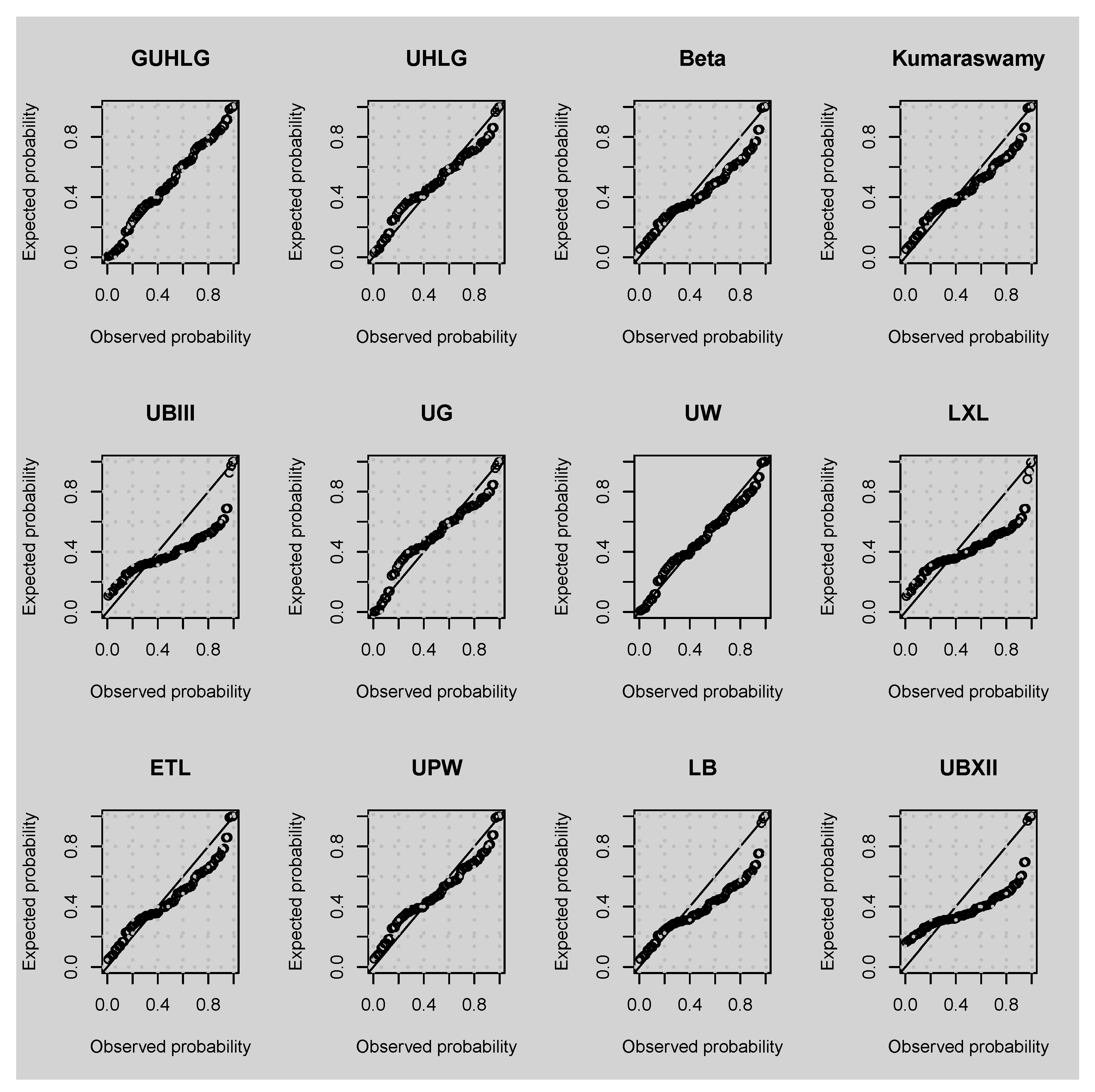
| Distribution | AIC | BIC | KS (p Value) | ||||||
|---|---|---|---|---|---|---|---|---|---|
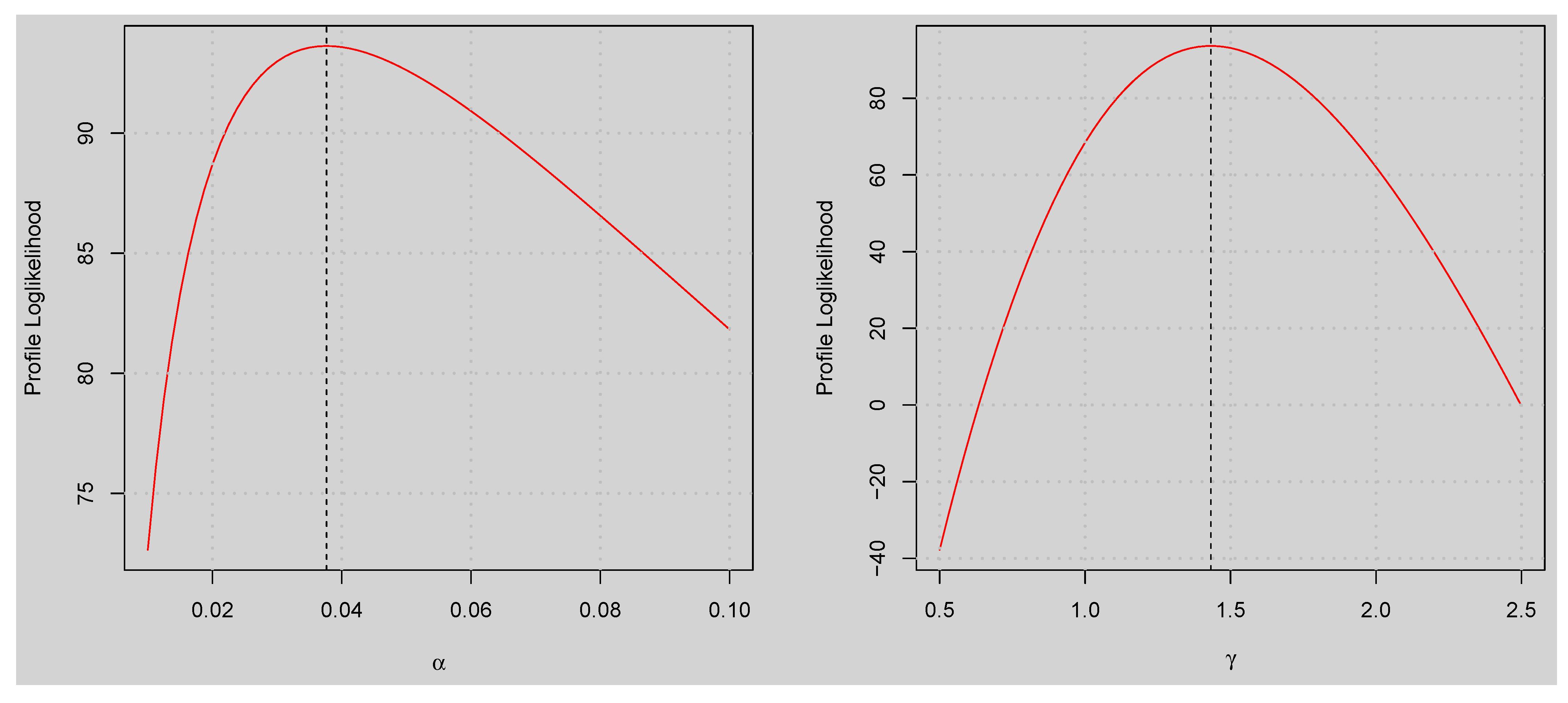
| GUHLG | 0.038 | 1.432 | −187.265 | −183.265 | 0.000 | 0.952 | −178.684 | 0.063 | |
| UHLG | 0.132 | −179.071 | −177.071 | 6.194 | 0.043 | −174.780 | 0.119 | ||
| Beta | 0.613 | 3.798 | −152.235 | −148.235 | 35.030 | <0.001 | −143.654 | 0.181 | |
| Kumaraswamy | 0.665 | 3.441 | −157.308 | −153.308 | 29.957 | <0.001 | −148.727 | 0.154 | |
| UBIII | 0.234 | 1.532 | −123.663 | −119.663 | 63.602 | <0.001 | −115.082 | 0.318 | |
| UG | 0.150 | 0.605 | −174.298 | −170.298 | 12.967 | 0.002 | −165.717 | 0.131 | |
| UW | 0.0655 | 2.353 | −176.201 | −172.201 | 11.064 | 0.004 | −167.620 | 0.093 | |
| ETL | 0.654 | 1.961 | −153.906 | −149.906 | 33.358 | <0.001 | −145.325 | 0.165 | |
| LXL | 0.500 | −129.518 | −127.518 | 55.746 | <0.001 | −125.228 | 0.304 | ||
| LB | 3.164 | −149.953 | −147.953 | 35.312 | <0.001 | −145.662 | 0.264 | ||
| UPW | 500.000 | 0.700 | 0.001 | −165.738 | −159.738 | 23.526 | <0.001 | −152.867 | 0.126 |
| UBXII | 0.348 | 2.841 | −93.013 | −89.013 | 94.252 | <0.001 | −84.432 | 0.338 | |
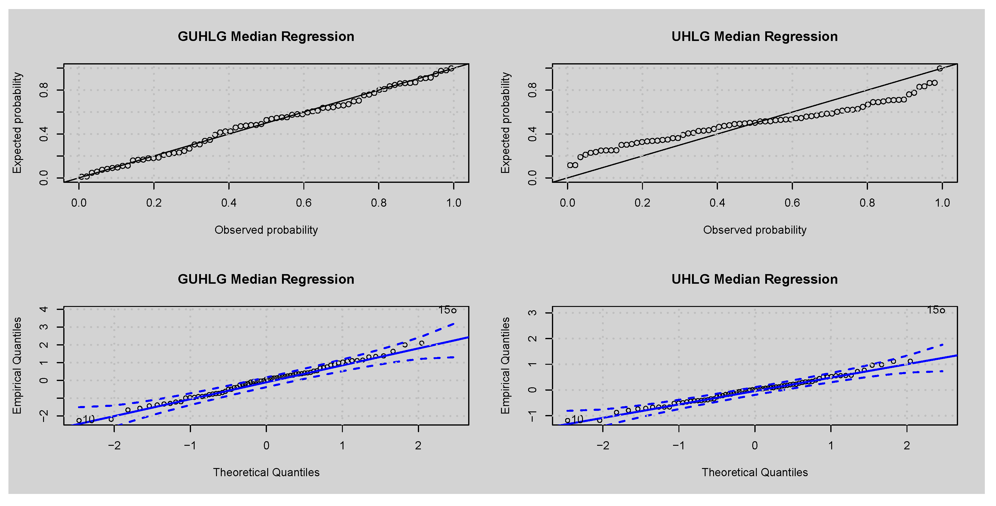
| Parameter | GUHLG Median | UHLG Median | ||||
|---|---|---|---|---|---|---|
| Estimates | Standard Error | p Value | Estimates | Standard Error | p-Value | |
| 3.985 | 1.211 | 0.001 | 4.128 | 2.067 | 0.046 | |
| −0.012 | 0.012 | 0.310 | −0.012 | 0.022 | 0.580 | |
| −0.053 | 0.223 | 0.814 | 0.018 | 0.404 | 0.965 | |
| −0.909 | 0.125 | <0.001 | −0.918 | 0.208 | <0.001 | |
| 2.343 | 0.623 | <0.001 | 2.145 | 0.909 | 0.018 | |
| −0.137 | 0.084 | 0.103 | −0.092 | 0.151 | 0.544 | |
| 0.009 | 0.020 | 0.635 | 0.005 | 0.036 | 0.895 | |
| 2.203 | 0.227 | <0.001 | ||||
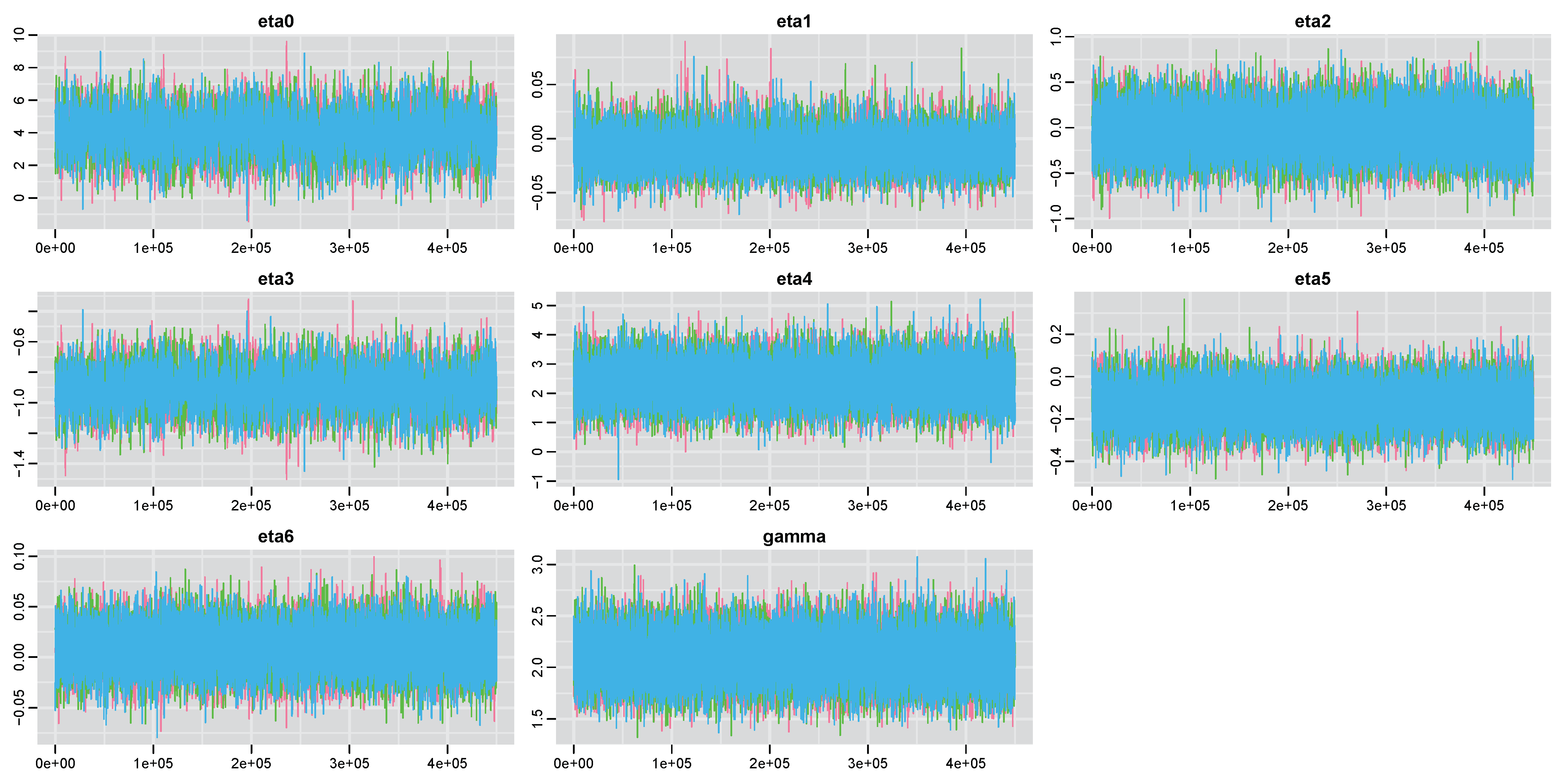
| Parameter | Estimate | SD | Naïve SE | 2.5% | 25% | 50% | 75% | 97.7% | neff | |
|---|---|---|---|---|---|---|---|---|---|---|
| 3.968 | 1.292 | 0.008 | 1.428 | 3.110 | 3.966 | 4.835 | 6.4835 | 1.001 | 15,000 | |
| −0.011 | 0.016 | 0.000 | −0.040 | −0.021 | −0.011 | −0.001 | 0.022 | 1.001 | 27,000 | |
| −0.046 | 0.240 | 0.002 | −0.509 | −0.208 | −0.049 | 0.116 | 0.430 | 1.001 | 27,000 | |
| −0.908 | 0.132 | 0.001 | −1.168 | −0.997 | −0.908 | −0.819 | −0.651 | 1.001 | 27,000 | |
| 2.373 | 0.657 | 0.004 | 1.111 | 1.927 | 2.368 | 2.806 | 3.690 | 1.001 | 27,000 | |
| −0.130 | 0.090 | 0.001 | −0.305 | −0.190 | −0.131 | −0.069 | 0.050 | 1.001 | 7000 | |
| 0.009 | 0.021 | 0.000 | −0.033 | −0.006 | 0.009 | 0.023 | 0.050 | 1.001 | 14,000 | |
| 2.078 | 0.225 | 0.001 | 1.654 | 1.924 | 2.071 | 2.227 | 2.537 | 1.001 | 27,000 |
Disclaimer/Publisher’s Note: The statements, opinions and data contained in all publications are solely those of the individual author(s) and contributor(s) and not of MDPI and/or the editor(s). MDPI and/or the editor(s) disclaim responsibility for any injury to people or property resulting from any ideas, methods, instructions or products referred to in the content. |
© 2023 by the authors. Licensee MDPI, Basel, Switzerland. This article is an open access article distributed under the terms and conditions of the Creative Commons Attribution (CC BY) license (https://creativecommons.org/licenses/by/4.0/).
Share and Cite
Nasiru, S.; Chesneau, C.; Abubakari, A.G.; Angbing, I.D. Generalized Unit Half-Logistic Geometric Distribution: Properties and Regression with Applications to Insurance. Analytics 2023, 2, 438-462. https://doi.org/10.3390/analytics2020025
Nasiru S, Chesneau C, Abubakari AG, Angbing ID. Generalized Unit Half-Logistic Geometric Distribution: Properties and Regression with Applications to Insurance. Analytics. 2023; 2(2):438-462. https://doi.org/10.3390/analytics2020025
Chicago/Turabian StyleNasiru, Suleman, Christophe Chesneau, Abdul Ghaniyyu Abubakari, and Irene Dekomwine Angbing. 2023. "Generalized Unit Half-Logistic Geometric Distribution: Properties and Regression with Applications to Insurance" Analytics 2, no. 2: 438-462. https://doi.org/10.3390/analytics2020025