

Dynamic Skyline Computation with LSD Trees †


M&D Data Science Center, Tokyo Medical and Dental University, Tokyo 113-8510, Japan
†
This article is an extended version of our paper published in the proceedings of the 17th International Database Engineering & Applications Symposium, IDEAS’13, Barcelona, Spain, 9–13 October 2013.
Analytics 2023, 2(1), 146-162; https://doi.org/10.3390/analytics2010009
Submission received: 31 December 2022
/
Revised: 24 January 2023
/
Accepted: 1 February 2023
/
Published: 9 February 2023
(This article belongs to the Special Issue Feature Papers in Analytics)
Abstract
:Given a set of high-dimensional feature vectors , the skyline or Pareto problem is to report the subset of vectors in S that are not dominated by any vector of S. Vectors closer to the origin are preferred: we say a vector x is dominated by another distinct vector y if x is equally or further away from the origin than y with respect to all its dimensions. The dynamic skyline problem allows us to shift the origin, which changes the answer set. This problem is crucial for dynamic recommender systems where users can shift the parameters and thus shift the origin. For each origin shift, a recomputation of the answer set from scratch is time intensive. To tackle this problem, we propose a parallel algorithm for dynamic skyline computation that uses multiple local split decision (LSD) trees concurrently. The geometric nature of the LSD trees allows us to reuse previous results. Experiments show that our proposed algorithm works well if the dimension is small in relation to the number of tuples to process.
1. Introduction
Dynamic skyline queries appear as common query types of recommender systems: walking tourists querying for restaurants with respect to price and distance, route planning systems on dynamic routing networks involving temporal congestions or road closures (e.g., [1]), online shopping portals with dynamically responsive input masks such as sliders for prices, sizes, and so on. All these use cases have in common that often a user does not issue a single query, but a sequence of queries, where successive queries only have slightly different parameters (movement of the tourists, the time passed in temporal routing networks, and the sliders of a webpage input mask). A naïve approach is to start the computation of the skyline set each time from scratch. Dynamic skyline algorithms provide fast results for recurring queries of the same kind by caching [2]. The key to dynamic skyline is a generalized mapping of the input data to the feature vector space. Instead of reconstructing this mapping for each query, it stays the same during recurring queries. Effectively, the vector space is parameterized by a query vector, i.e., it is shifted by an offset.
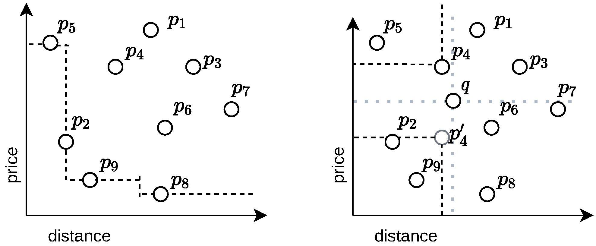
Let us examine a concrete example with the feature vectors . The answer to the classic skyline problem (the query vector is ) is the skyline set , because all points in this set are incomparable (i.e., none of them dominates each other), while the remaining elements such as are dominated by one of the elements of the skyline set (e.g., dominates ). In the classic skyline problem, we regard vectors closer to the origin as better than others that are farther away in all dimensions. A geometric interpretation is to connect the skyline set with line segments such that all points to the upper right of these line segments are dominated. See Figure 1 for a geometric interpretation, which we keep as a running example in this article.
The skyline set changes if we shift the origin as we are allowed to do in the dynamic skyline problem. Let us select as an example. Then the skyline set is , and the answer remains unchanged when shifting q to or . For instance, is dominated by because and , and the absolute value of the difference in both dimensions is smaller for than for . With Table 1, it is easy to verify the calculation.
It is easy to see that a naïve computation of the skyline set involves comparing each vector with all other vectors. Assuming that we can compare two vectors in in time, we can compute the skyline set in time, where m is the input set size. The question we pose in this article is whether we need to compare all elements with each other, and whether a recomputation for a different query point is needed. To this end, we review an algorithm using a geometrical data structure, called the LSD tree, which leverages geometric distributions and is in favor of pruning subsets of the input in certain cases. This tree data structure also gives us means for reasoning about when a recomputation of the dynamic skyline set is necessary.
1.1. Dynamic Skylines
Consider a data set and a scoring function . We call an elements a tuple, and its respective (feature) vector. (Instead of directly working on feature vectors, by mapping the input element to feature vectors, we can support the case that multiple elements can have the same feature vector, i.e., we allow the geometrical representation of tuples by not necessarily distinct feature vectors.) Let us say that we have a query vector and want to compute the dynamic skyline of q [3], i.e., we want to find all vectors of that are not dominated by any other vectors with respect to q. We say a vector dominates another vector if its distance to q has an equal or lower value than the other vector’s distance to q in all respective coordinates, and a strictly lower value in at least one coordinate. According to this definition, the query vector always dominates all other vectors, but q is not part of in general. We call q an offset vector because it moves the best location of the classical skyline problem to its own location (e.g., we translate the vector space by ). Vectors are often illustrated as points of the vector space equipped with the norm, given by for . The latter is useful, as two distinct vectors are incomparable with respect to domination when their norm is equal. For instance, and are feature vectors in with and therefore both are incomparable.
1.2. Structure of the Paper
In what follows, we tackle the problem of answering dynamic skyline queries. Given a data set , we precompute a data structure based on LSD trees, such that for a sequence of query points , we can use this data structure to quickly answer , and reuse this answer for computing if possible.
To this end, we study a modification of the Skyline Breaker algorithm [4] using LSD trees. While the original paper suggests an algorithm for classic skyline computation, we extend its usage to dynamic skyline queries. Therefore, we review the main ideas before addressing our new enhancements. The rest of our paper is organized as follows: Section 2 contains an overview of related work with regards to skyline computation on tree data structures. We introduce basic definitions and helpful lemmata in Section 3 with the sLSD tree structure in Section 4 before focusing on the algorithm itself in Section 5. There, we present the problem and highlight different techniques for optimizations. Finally, Section 6 reflects possible performance speedups and slowdowns.
2. Related Work
Computing the skyline by means of geometric representation of data already produces many results. Kossmann et al. [5] proposed nearest neighbor (NN) search operating on an R*-tree [6] structure. This idea was extended by Papadias et al. [7], featuring the branch-and-bound skyline (BBS) algorithm. They were also the first to propose the dynamic skyline problem [3]. Using the M-tree [8] as a geometrical representation for the data, Chen and Lian [9] reasoned about pruning techniques for fast dynamic skyline computation. In addition to providing a dynamic skyline algorithm, Sacharidis et al. [2] proposed caching methods to speed up computation in subsequent queries. Recent research approaches can compute the dynamic skyline for massive datasets [10], work in parallel [11], or work on distributed systems [12]. Along with new proposals for skyline computation, the focus of recent research projects tends to parallelization of classic skyline algorithms. Selke et al. [13] discussed a variant of block-nested loop (BNL) using the Lazy List [14] data structure. Techniques like optimistic locking are shown as a good trade-off between redundant synchronization steps and race conditions. By doing so, they manage to successfully shrink the sequential fraction of BNL. A parallelized variant of BBS has been proposed by Im et al. [15]. Obviously, dynamic skylines and parallel skyline algorithms are part of an active research area. The combination of both fields is the topic of this paper.
A related problem, but not studied in this paper, is to allow the underlying dataset to be dynamic. Considering dynamic datasets, Essiet et al. [16] studied multi-objective optimization; Hu et al. [17] proposed routing on dynamical environments; and Gulzar et al. [18] gave an algorithm for computing the skyline by pruning and selecting superior local skylines (see also references within the PhD thesis of Alami [19]).
3. Preliminaries
As in common calculus, denotes the projection to the i- th coordinate, i.e.,
We call a function a scoring function. Here is a subset of an arbitrary universe. Further, for a scoring function , we call the feature vector of . So that there is no possibility for confusion, we write to express the cardinality of a set S, i.e., the number of elements of S.
Scoring and Dominance. In what follows, we first consider a fixed offset , which represents our query point. The motivation for the definitions is that f and q induce a strict weak ordering on , called a dynamic scoring of . For two vectors , we call v better than w with respect to q if there exists a such that and for every . We write for short. Analogously, we write for two tuples if and only if holds. We can put this statement the other way around: if there is no such that , then either or y dominates x.
For instance, given two data points and with and , then and . For , we have that , whereas for , because and .
Formal Problem Definition. The dynamic skyline parameterizes the classic skyline by feature vector q as an offset [3]. More concretely, the dynamic skyline set holds the condition
We also call a tuple that is not dominated by any other tuple of , or more briefly, we call x a skyline point (if the context with and q is clear). In the following, when the sense is obvious, we identify a tuple with its value , e.g., we do not explicitly mention any notion of f. So when speaking about coordinates of x, we actually mean the coordinates of .
Lemma 1.
Let be a cover of , i.e., . Then
Proof.
Let , then for all , there either exists a such that . Hence . □
4. The sLSD Tree
The LSD tree is a hybrid tree that has bucket nodes as leaves and directory nodes as internal nodes. Dictionary nodes have always two children, and therefore an LSD tree is a full binary tree. Bucket nodes are the actual nodes that store the data.
In the beginning, the tree consists of a single bucket node. Whenever a bucket node contains more than M elements, this bucket node will be split. In our case, the split point is determined by the median of all elements according to one dimension. After the split, we have a left and a right bucket node: the left bucket contains those elements that have smaller values than the split position in the split dimension. The information about the split is saved in a new directory node that replaces the previous bucket node and adopts both new bucket nodes as children. We can consider a dictionary node as a separation of its two bucket children with a hyperplane. While bucket nodes store the actual data, a directory node only saves the split position and the two bucket nodes split by this hyperplane. Figure 2 gives an example.
Exactly as the kd tree [20], the split dimension can be determined by the tree-depth of the bucket node that was split. In another perspective, the LSD tree partitions data of into disjoint cuboids where each cuboid contains all elements of exactly one bucket. Each bucket can therefore be represented as a cuboid whose coordinates are saved in the ancestor nodes’ split positions. We call this particular cuboid the bounding cuboid of the bucket. Computing the nearest neighbor (NN) of an arbitrary point is done by the following steps: First, traverse the tree in a top-down manner in order to locate the bucket in which q would belong. Next, recursively climb the tree upwards while scanning the sibling node at each depth for near points. If this sibling is an internal node, we additionally scan its subtree recursively. Henrich [21] proposes an algorithm that takes the distances to already found points for a bound to stop the naïve search prematurely. The difference between the LSD tree and our sLSD tree is the lack of external directory nodes as we restrict the problem for in-memory use cases.
4.1. Dealing with Skewed Distributions
The sLSD tree splits an overfull bucket by sorting its elements in a certain dimension and taking the median. For a kd tree, the split dimension of a bucket is usually the split dimension of its parent node, shifted by one, i.e., if the parent node has a split dimension d, then the bucket gets split at dimension . In the worst-case scenario, all elements share the same value in this dimension. A split would therefore create two new buckets: one assigned with the entire content and the other left empty. Henrich [22] avoids this bad behavior by simply iterating over the split dimension until he finds different values of the elements in this dimension. For termination, we just have to check if at least two elements have different feature vectors. Another method would take those dimensions into account as a split dimension, for which only a few objects’ values collide with the median value in this dimension. If there are multiple dimensions with the same number of minimal collisions, then we take the dimension with the highest variance of feature vector values out of this remaining set. This additional filter tries to hinder any bucket from becoming too elongated in specific dimensions.
4.2. Complexity Analysis
As a member of the kd tree family, the sLSD tree shares complexity traits with its ancestor. In fact, the kd tree is a specialization of the sLSD tree with a maximum bucket size of . On the one hand, for negligibly small M, the sLSD tree provides operations like inserting or locating an element in average and worst time. On the other hand, an lets the sLSD tree store the entire data in a single bucket. Hence, the time complexity is based on the data structure used for the buckets. For the other cases with , we have to take care with the more complex insertion step. If we assume contrarily to Section 4.1 that the median value is always unique under all considered objects during a split, then any split of an overfull bucket at the median creates two buckets, each containing at least elements. Moreover, our algorithm will not remove any element of the sLSD tree. After inserting elements, there is at no time any bucket with less than elements. Let us use the random variables with for counting the elements of each bucket of an sLSD tree with k leaves. These variables satisfy the constraint that . In the average case, the occupancy rate is distributed uniformly over all intervals, hence we get , i.e., . Therefore, the sLSD tree has an average depth of . The costs for inserting an element are a combination of
- finding the bucket in which the element shall be inserted; the time is logarithmic in the depth of the tree; and
- splitting this bucket if it is overfull. The split is done by
- (a)
- sorting the elements in one dimension that takes time, and
- (b)
- creating a new bucket that takes time for moving half of the elements to the new bucket.
Overall, a newly created bucket can take new elements on average before it has to be split. Hence, this step takes amortized time.
To sum up, insertion takes amortized time on average. In the worst case, all buckets have minimal occupancy, i.e., . Thus, we have . Let us take an empty sLSD tree. If we insert a sequence of elements that are strictly ordered, we obtain, as for kd trees, a caterpillar tree with the worst-case depth of if we drop the constraint of unique values for determining the split dimension (i.e., all feature vectors must not have the same value in the split dimension). It is easy to see that the distribution of elements will affect not only the number of buckets, but also the time complexity. Fortunately, Henrich [23] provides a heuristic online strategy that tries to redistribute the occupancy. His strategy tries to shift the split position of the parent node of an overflowing bucket in order to prevent the split of the bucket. However, we have to take into account what kind of node the sibling of the brimful bucket is:
- If the sibling is a bucket that has space left, we just shift the parent node’s split position such that the number of elements gets rebalanced.
- If the sibling is a subtree that can adopt a new element without splitting one of its children, we shift again the split position of the bucket’s parent node. This time, however, we also have to recompute the split information of the internal nodes of this subtree.
If none of these conditions can be applied, we declare the bucket’s parent node as overfull and try to shift the split position of its respective parent. Hence, if a local redistribution is not possible, we recursively go up the tree and reconstruct the split information. Regarding aggressive shifting strategies, there is a certain trade-off between overall bucket utilization and the number of directory nodes [23].
4.3. Geometrical Characteristics
In the context of the Skyline Breaker algorithm, we are particularly interested in catching skyline points out of the sLSD tree quickly. Therefore, we need to compute the bounding cuboids for nodes with arbitrary depth. For that, we denote with the depth of any node e of an sLSD tree. The following lemmas will help us to solve this task.
Lemma 2
([4]). Let b be an arbitrary leaf node. To determine the bounding cuboid of b, we need to examine n ancestors of b.
Let us recall that is our query vector.
Lemma 3.
Let be a feature vector. The pairwise disjoint, non-bounded cuboids do not contain any skyline point, where . Furthermore, is connected.
Proof.
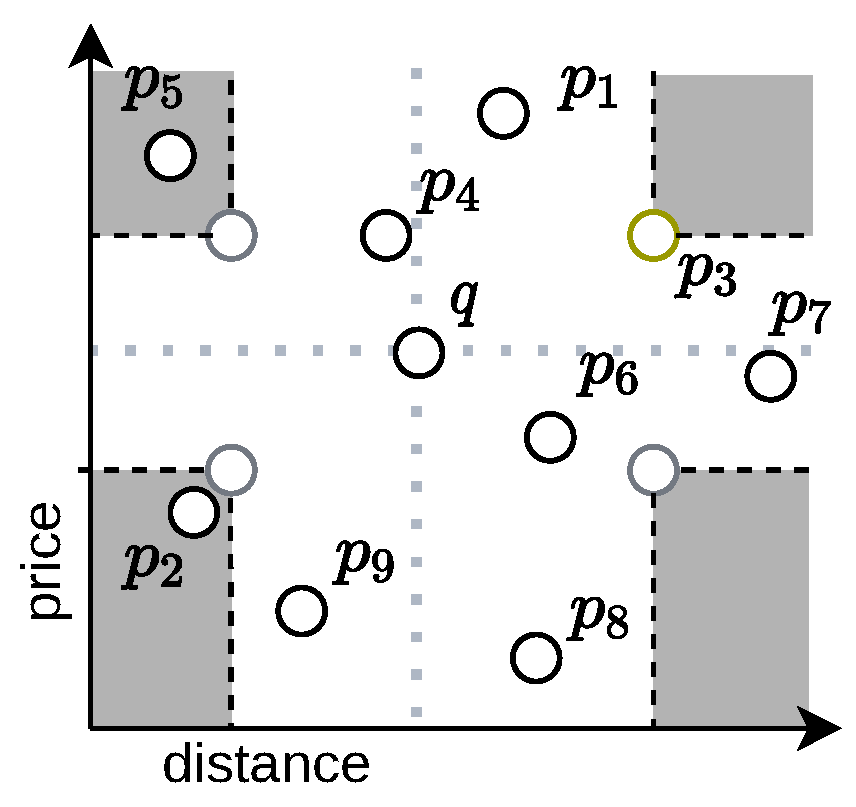
For every feature vector , we have for every , and thus u is dominated by o. See Figure 3 for an illustration. Since all cuboids are pairwise disjoint, and each point v that is not dominated by o is not in , we conclude that is connected. □
Lemma 4.
Both the siblings of and the descendants of ’s ancestors with depth at least can contain skyline points.
Proof.
Without loss of generality, we assume . Let p be the ancestor of with a depth of , and let c be the child that is the ancestor of . The node c has a depth of . The descendant directory nodes of c and c itself cannot have any split position farther away from q than p. Otherwise, the bucket would be at a different location than q. Because of the definition of , no directory node that is both ancestor of and descendant of p has the split-dimension of p. Hence, there is no leaf node of c whose bounding cuboid is contained (entirely) in D (due to Lemma 3 with ). □
5. The Algorithm
While the original algorithm restricts itself to non-negative feature vectors, we had to relinquish this constraint in order to parameterize the skyline computation with an arbitrary offset q. Therefore, we reintroduce basic original concepts while providing our alterations.
5.1. The Dynamic Skyline Breaker Algorithm
We generate an sLSD tree for each thread. Each thread starts with the SBDyn (Algorithm 1) immediately after its tree is filled with the input data. Firstly, we search the nearest neighbor of q with respect to the norm in terms of bucket nodes by Henrich ’s distance-scan algorithm [22]. While locating this node, at most buckets have to be examined. Because we have not yet found any dominator, these buckets might contain skyline points in addition to a. Hence, we collect these buckets for local skyline computation and call them for some I. Let be a NN of q, and let denote the bucket in which q would be added. Now, having Lemma 2 in mind, we start to traverse the tree reversely, counting our steps upwards. We initialize a vector that keeps track of the geometric position. While climbing the tree upwards, we examine the sibling c of the node we came from. If we have not counted upwards to the dimension n, at least one of v’s coordinates is zero (see Lemma 4). Therefore, we cannot discard c. In other words, we need to traverse c and collect all of its buckets. When we have reached the number n with our counting, one of the descendants of c could be discarded. That is because some descendants’ buckets might be contained in the region without skyline points considered in Lemma 3. Therefore, we start a new task that traverses c, done by the tree clipping described in Section 5.3 and Algorithm 2. We have traversed the tree when we have reached the root node while climbing up the tree from . The last step is the allocation of the global skyline. For overview, we present a flow chart of the algorithm in Figure 4.
| Algorithm 1 Dynamic Skyline Breaker: The ternary ? operator has the same semantic as in C/C++, i.e., means if a then b else c. |
| 1: function sbDyn() |
| 2: |
| 3: |
| 4: |
| 5: |
| 6: |
| 7: for do |
| 8: |
| 9: |
| 10: |
| 11: while do |
| 12: |
| 13: |
| 14: if then |
| 15: |
| 16: else |
| 17: |
| 18: |
| 19: |
| 20: clip() |
| 21: return |
| Algorithm 2 Clipping the Tree |
| 1: function clip() |
| 2: |
| 3: |
| 4: |
| 5: if then |
| 6: |
| 7: else |
| 8: |
| 9: |
| 10: |
| 11: if then |
| 12: |
| 13: if then |
| 14: |
| 15: else |
| 16: |
5.2. Skyline in a Bucket
For local skyline calculations, we can modify any skyline algorithm to work with an offset of q. We did this with a simple BNL-based algorithm that works directly on the bucket, while subtracting the offset ahead of comparison.
5.3. The Tree Clip Algorithm
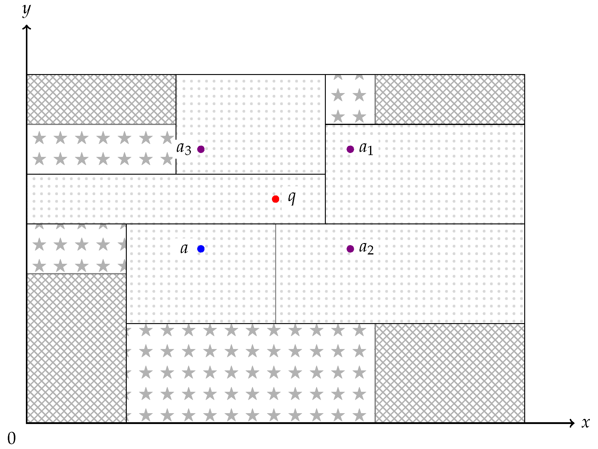
Algorithm 2 works with a divide-and-conquer (DC) strategy. We start with a directory node and the split information of its parent node. It is advisable to hold these data in a variable by setting the coordinate entry of p at the split dimension to the split position, while all other coordinates are kept identical to q’s position for a start. The other child c of our current directory node can be illustrated as a cuboid with the corner point that is closest to q. Therefore, while we traverse the children of our current directory node, we note down the split information in v until we have gained coordinates for all dimensions. With this information represented by the split point , using the condition , we now check whether discarding the child node c is feasible. If the condition holds, we know that all elements contained in the cuboid of c are dominated by a. Thus, we discard the node c, even if it is a directory node. Otherwise, we have to traverse the right node recursively, again denoting its split data. Figure 5 gives a geometric interpretation of an LSD tree, where we have located the bucket of q and a bucket containing a.
Remark 1.
According to Lemma 4, if the depth of the sLSD tree is less than , we cannot make use of the clipping technique.
6. Analysis and Optimization
Let us retrace the versatile steps involved in the algorithm while analyzing the time complexity. At the start, locating takes time on average and time in the worst case, according to Section 4.2. Subsequently, a is found while examining at most that takes time in the worst case. If we take a balanced sLSD tree for granted, the preparation step of Section 5.3, which moves upwards until reaching at least n different dimensions, will also take buckets into consideration. For local skyline computation of any bucket of size , an algorithm like BNL [24] applied in Section 5.2 needs at least time (assuming that it is left to compare all feature vectors by a single remaining dimension at which they differ) and has worst-case time complexity. The time taken by the actual tree clipping algorithm is heavily dependent on the distribution of split information and takes at least the time proportional to the remaining depth of the current node in the sLSD tree after the preparation step. By building our algorithm on the sLSD tree, we obtain a hybrid approach that employs both the DC strategy of Section 5.3 and some nested-loop algorithms of Section 5.2. Both strategies are weighted by the maximum bucket size M. On the one extreme, for , we get a kd tree-like structure with singletons as buckets. According to the complexities of Section 4.2, setting creates a much larger tree structure and exploits entirely the DC strategy. On the other hand, taking any puts the entire content in a single bucket and just evaluates the nested-loop algorithm. For taking advantage of both algorithms, a has to be chosen, dependent of the input data’s distribution. Obviously, there are data sets for which choosing a small or large M results in a speed-up. A best-case scenario for large M is a correlated data set with time complexity for the BNL of any subset . If the sLSD tree is balanced, we have a depth of and thus leaves. Hence, the algorithm will take at most time. On the other hand, extremely anti-correlated data can pose the worst-case running time for the BNL. However, if the clipping condition holds for most of the time, we have for the best case running time for the tree climbing algorithm that collects buckets of a balanced LSD tree in addition. For merging these buckets, we have for a best-case and for a worst-case time. Note that both times are independent of . Hence, we argue that the dimensional factor plays only a minor role for a reasonably large .
Proposition 1.
The Skyline Breaker algorithm accesses the optimal number of nodes for computing the dynamic skyline set of q, i.e., no algorithm will solve the same problem while visiting fewer nodes on the same data structure without knowledge of the contents of any bucket.
Proof.
Let us assume that our algorithm unnecessarily inspects a bucket u that can be safely pruned. The bucket u has a bounding rectangle with corner points . Let be a best corner, i.e., for every . In the contrary, there has to be an element with . Otherwise, without further knowledge, we have to inspect the bucket u. We also know that the NN of q is always part of the skyline set. Hence, every algorithm that computes the dynamic skyline set has to access the bucket that would take a as a new element of the global skyline. Due to the fact that Algorithm 2 traverses the tree from upwards, we will encounter nodes in an ascending, weakly-sorted order with respect to its best corner. In other words, the algorithm will either find a bucket containing v before accessing u or find a bucket that dominates v. In both cases, we will not inspect the bucket u; we clip either a subtree containing u or u itself. □
7. Comparison to Other Geometrical Data Structures
Our usage of the LSD tree is motivated by modern computer hardware architectures featuring large caches. While the well-known kd tree can be seen as a special case of an LSD tree with a bucket of size 1, large bucket sizes leverage cache effects: for the skyline computation within a bucket, we stick to a basic block-nested loop algorithm with a naïve time complexity of . However, this algorithm is practically fast if it operates on data within the cache size of the CPU. Additionally, parallel evaluation is easy since the dominance check for each element can be performed independently. In that sense, large bucket sizes shrink the height of the LSD tree compared to the kd tree while spending only a negligibly additional cost for the computation within the relatively large buckets. Another well-known geometric representation is an r tree [25]. Since the internal node of an r tree stores the complete geometric information about its bounding cuboid, computing this information is cheap compared to our approach with the need to have a node-to-ancestor path of length n to have the split information for all n dimensions. Nevertheless, skewed distributions of the input can cause inefficiencies like empty or mostly empty cuboids. It can also often happen that cuboids intersect such that it is harder to detect whether pruning of nodes can be done.
7.1. Improving the Clipping Condition
The tree clipping (Algorithm 2) could be extended to use a list of known skyline points instead of solely a (a as defined in Section 5.1). A large list of global skyline points reinforces the clipping in Section 5.3 by testing for any instead of only a. Thus, a skyline subset will provide a higher chance of clipping. Actually, we can already enlist some points while finding a; let us recall that the search for the NN of q can take at most buckets into account. Due to the distance-scan algorithm [22], each of these buckets is a neighbor of . A potentially huge number arises from the number of orthants that are spawned by q (see Lemma 3). Because the bounding cuboids form a connected region that contains q, there exists a certain area in which we can be sure that local skyline points belong to the global dynamic skyline . More precisely, we compute the maximal cube (i.e., a cuboid with equal sides) that is contained in the union of all buckets. We denote its side length with s. Then any with is in the global skyline . If there is a , then and hence , a contradiction for o being a local skyline point. By taking any as-yet encountered local skyline point for filtering during the clipping, Proposition 1 is tightened to the statement that the algorithm is optimal with respect to the class of algorithms that may also use knowledge of the buckets’ contents.
7.2. Analysis of Parallelism
At first glance, it seems an easy task to divide the algorithm into independent subtasks: firstly, the input data are partitioned and each part gets processed by a different thread. Particularly for a concurrent input source like data stored in the RAM of a CRCW (Concurrent Read Concurrent Write) machine, there is no sequential bottleneck. In the main step, each thread computes independently the skyline of its fetched input data. Finally, we just merge the local skylines until a single (i.e., the global) skyline remains. Unfortunately, the described algorithm is not embarrassingly parallel; it has several delicate parts that we have to take care of when adding concurrent structures to our code. In particular, this involves the queue that holds the computed, local skylines. For this job, Java 7’s ConcurrentLinkedQueue with wait-free access support [26] seemed fitting for us. Moreover, before climbing up its LSD tree, every thread must have at least one close neighbor of q in order to make use of the clipping technique. This may be either a point of the thread’s own input data set, a global NN of q, or even a list comprising every already found skyline point. Hence, we either use a global synchronization barrier (meaning all threads wait for a global communication process to start) or a concurrent list that is filled with newly found local skyline points and trimmed when an already stored point gets dominated by a recently collected point; this point cannot be dominated by another point from the list, otherwise the trimmed point would have been trimmed in advance. The other parts of the implementation can be written in the MapReduce and Fork/Join model. Both are two different models for parallel execution. They share the common goal of easing parallelization of a given sequential task. Nevertheless, their field of application is orthogonal. While MapReduce targets distributed computing, Fork/Join works merely on a single node. We describe our algorithm as a hybrid approach that employs both models—MapReduce for distributing the work-load to different nodes and Fork/Join for local multi-threaded computation. For the latter, we just translate the ideas of [4] to dynamic skyline computation. In order to describe our idea in the MapReduce framework, let us take a partition of , i.e., with for pairwise different. The three functions for each pairwise different subsets with any , and represent the common work flow of our MapReduce application. In particular, our implementation is a deterministic, multi-threaded program [27] because its schedule is predetermined by a fixed number of tasks that consists of the starting threads and the threads that combine the local skylines. Nevertheless, the code of SubSection 5.3 is non-deterministic with respect to thread spawning. That is caused by the fact that the number of tasks is dependent on the effectiveness of the clipping and the recursive divide-and-conquer technique. The latter tells us that the tree clipping is a fully-strict computation [28]. Because common frameworks like Hadoop do not allow dynamic task creation [29], the clipping cannot be described in terms of the MapReduce model. Fortunately, translating this part of the algorithm to the Fork/Join model seemed the right choice; Blumofe et al. [30] showed that the work-stealing technique is optimal for scheduling fully strict computations.
7.3. Caching Dynamic Skylines
The construction of the sLSD trees in Section 5.1 is done on the fly, i.e., the tree is not getting rebalanced during the initial bulk insertion of the data tuples . For reuse, we can restructure the sLSD trees to prevent worst-case scenarios for the subsequent queries. Therefore, we exchange our median-based split strategy with a distribution-dependent one [31] in order to cope, for instance, with skew-distributed data. An optimal refactoring of the tree results in a balanced tree with depth. Additionally, we save after each query the offset vector q along with its dynamic skyline set for reuse [2]. For effective caching, we have to introduce the notion of orthants of q:
Definition 1.
The offset q splits the space into orthants. If we give each orthant a number, we can write the j-th orthant of q as for every . By Lemma 1, we have .
Now, Proposition 1 and a variation of ([2], Lemma 2) comes in handy:
Lemma 5.
Let be an old offset and b a node of the sLSD tree whose bounding cuboid belongs to the j-th orthant of , but does not contain any points of the j-th orthant skyline set . If q is an offset and belongs to the j-th orthant of q, then b does not intersect with and thus can be clipped.
The cache is used to provide additional conditions for the clipping algorithm. Before employing the cache, we take only these elements into consideration that effectively help clipping:
Corollary 1
([2]). Let and be two old queries for which we have cached their results. If , then elements of the dynamic skyline set of are either part or dominated by elements of . Hence, will not clip additional nodes of the sLSD tree.
7.4. Evaluation
For the following evaluation, we used the implementation of the Skyline Breaker [4] algorithm, called SB in the following, which is freely accessible from https://github.com/koeppl/skylinebreaker (accessed on 30 December 2022). This implementation is written in the Java language. In this evaluation, we used the SBQuick class applying the pruning technique on the LSD trees with parallel threading. To compare our solution with other skyline algorithms, we used the skyline benchmark software of Wiemann [32] (https://github.com/sven-wi/SkylineCompare) (accessed on 30 December 2022). Upon request, we received Java implementations for pskyline and parallelBBS of Im et al. [15] written in this framework. While pskyline applies MapReduce on lists of tuples, parallelBBS is based on the algorithm of Papadias et al. [7] using r trees as the geometric representation of the data (cf. Section 7).
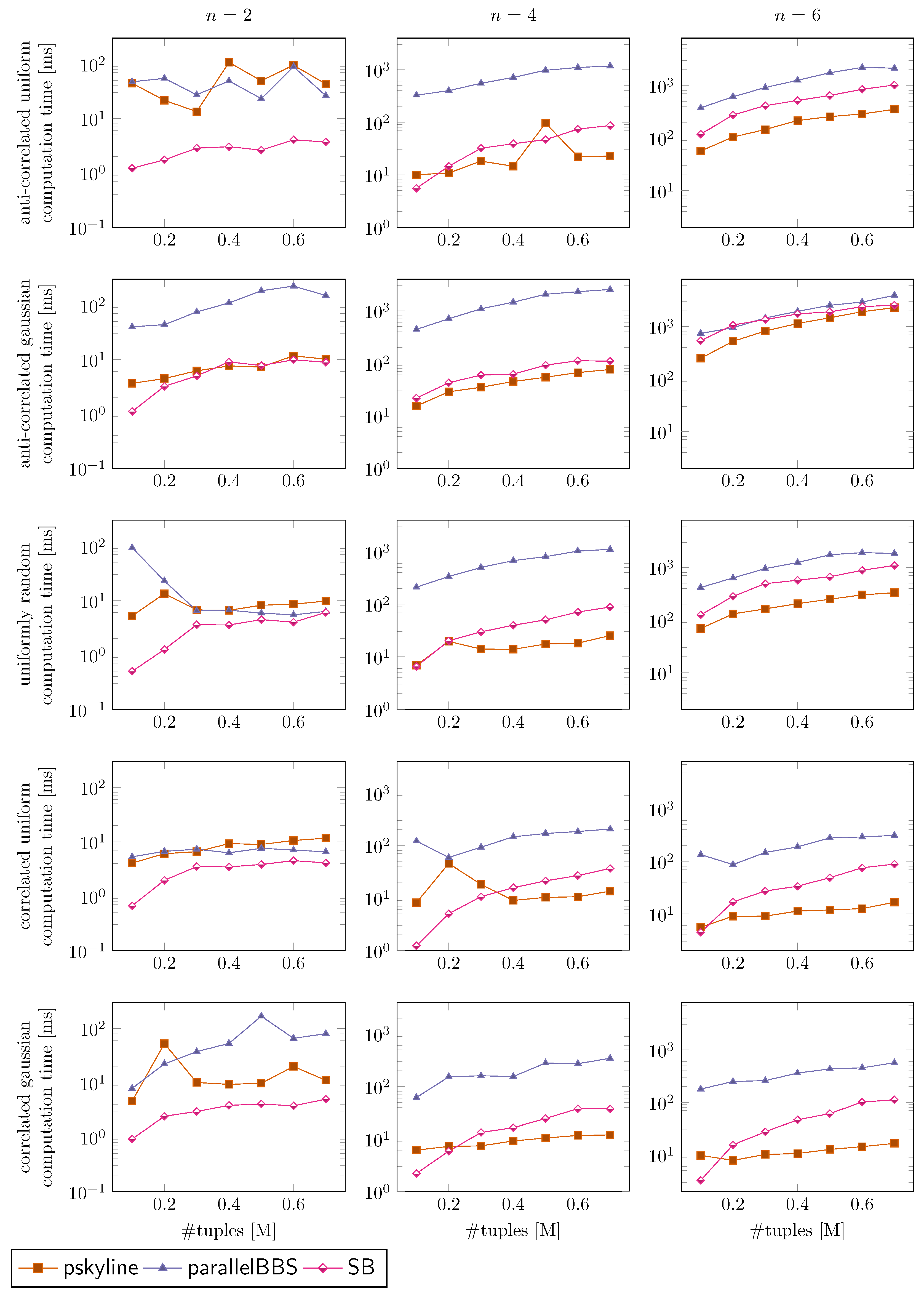
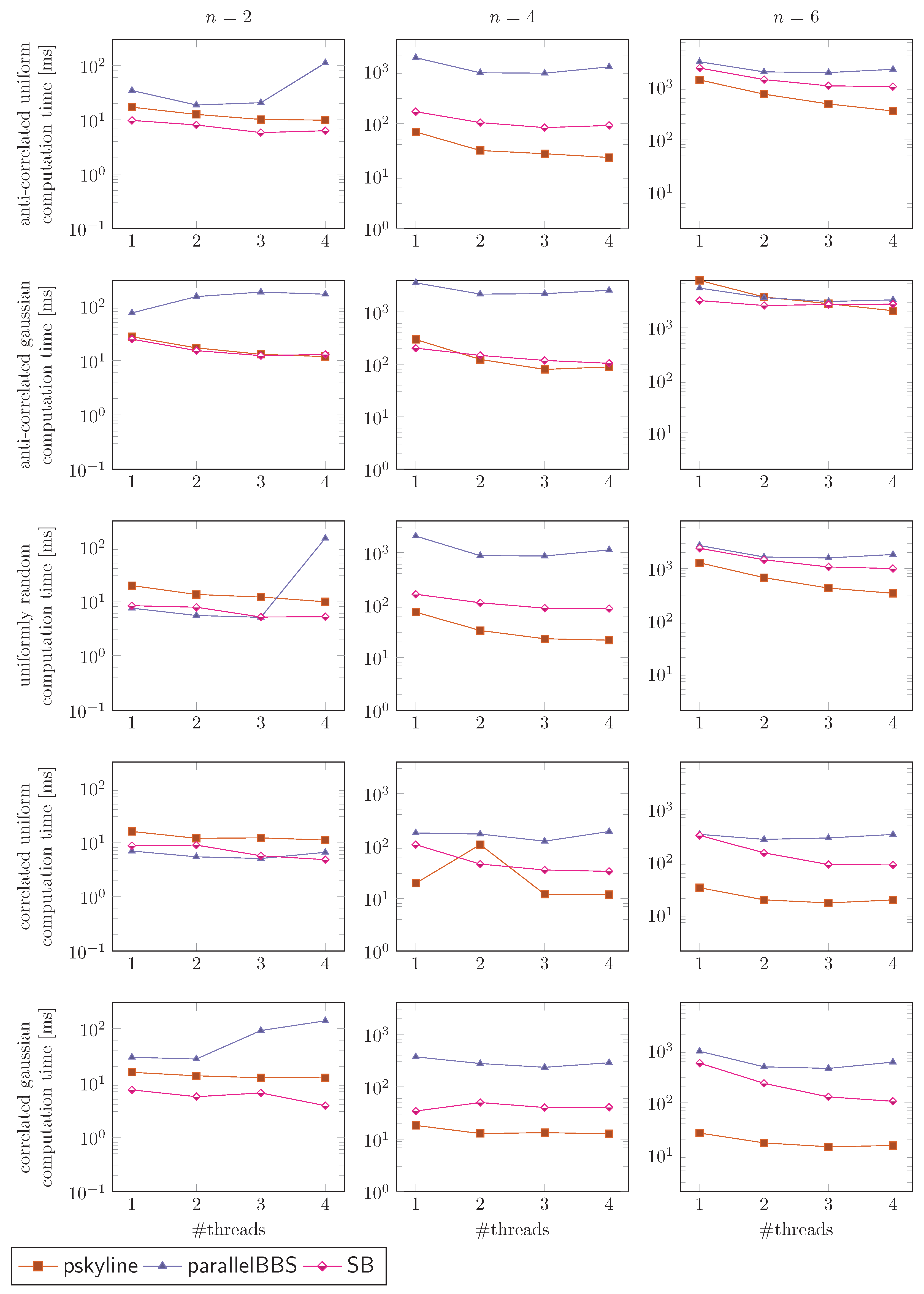
We ran our experiments on a Debian 11 machine with 128 GB of RAM and an Intel Core i3–9100 CPU with four cores. The experiments are split into two parts. In the first part (Figure 6), we scale the number of input tuples while evaluating the parallel algorithms with four threads. In the second part (Figure 7), we scale the number of threads from one up to four. In both parts, we select different correlations of the input data, which are randomly generated by the framework based on the dataset generation of ([24], Figures 10–12).
Overall Evaluation. We observe that SB excels at small dimensions for which we can quickly detect the boundaries of a bucket. For larger dimensions, the times for these checks become longer, and thus the overall performance deteriorates with n more than the performance of the other solutions. Following the curves while scaling the input, we observe that SB is still in the competitive range with the other solutions, yet not the best choice if we want to evaluate pure skyline queries. In all different distributions, we observe a similar progression of SB’s time curve, which supports the claim that the usage of the LSD trees as geometric data structures makes the algorithm robust against different data distributions.
Parallel Evaluation. When scaling the number of threads, we observe that SB becomes faster most of the time or stays roughly at a constant speed level. Other implementations deteriorate at several instances, becoming slower with a higher number of threads. We can conclude that SB is suitable for the computation of the skyline set in parallel.
8. Conclusions
We studied a geometrical interpretation of the dynamic skyline problem by using LSD trees. LSD trees have shown in practice that they can handle high-dimensional feature vectors with low impact on the input data’s distribution. For the skyline computation, we made use of an already existing algorithm, the Skyline Breaker algorithm. Some parts of the parallel algorithm were changed in order to cope with the dynamic version of skyline computation. The theoretical evaluation addresses the combinatorial nature of the algorithm and treats both best- and worst-case scenarios with respect to different maximum bucket sizes. Computing the boundaries of a selected bucket is easy in small dimensions since it involves visiting only some closest ancestor nodes. Unfortunately, the boundary computation has an exponential dependency on the dimension such that the approach can quickly become less appealing if the dimension is relatively high compared to the input size. In that case, we have seen in the experiments that other approaches are more suitable.
Funding
This work is funded by the JSPS KAKENHI Grant Numbers JP21H05847 and JP21K17701.
Institutional Review Board Statement
Not applicable.
Informed Consent Statement
Not applicable.
Data Availability Statement
The generated datasets in the experiments can be regenerated with the skyline benchmark software of Wiemann [32].
Acknowledgments
We thank the participants of IDEAS 2013 for drawing our attention to the dynamic skyline problem.
Conflicts of Interest
The author declares no conflict of interest.
References
- Köppl, D. Inferring Spatial Distance Rankings with Partial Knowledge on Routing Networks. Information 2022, 13, 168. [Google Scholar] [CrossRef]
- Sacharidis, D.; Bouros, P.; Sellis, T. Caching Dynamic Skyline Queries. In Scientific and Statistical Database Management; Springer: Berlin/Heidelberg, Germany, 2008; Volume 5069, pp. 455–472. [Google Scholar] [CrossRef]
- Papadias, D.; Tao, Y.; Fu, G.; Seeger, B. Progressive skyline computation in database systems. ACM Trans. Database Syst. 2005, 30, 41–82. [Google Scholar] [CrossRef]
- Köppl, D. Breaking Skyline Computation down to the Metal—The Skyline Breaker Algorithm. In Proceedings of the 17th International Database Engineering & Applications Symposium, IDEAS’13, Barcelona, Spain, 9–13 October 2013. [Google Scholar] [CrossRef]
- Kossmann, D.; Ramsak, F.; Rost, S. Shooting Stars in the Sky: An Online Algorithm for Skyline Queries. In Proceedings of the 28th International Conference on Very Large Databases, VLDB’02, Hong Kong SAR, China, 20–23 August 2002; Morgan Kaufmann: Burlington, MA, USA, 2002; pp. 275–286. [Google Scholar]
- Beckmann, N.; Kriegel, H.P.; Schneider, R.; Seeger, B. The R*-Tree: An Efficient and Robust Access Method for Points and Rectangles. In Proceedings of the 1990 ACM SIGMOD International Conference on Management of Data, SIGMOD ’90, Atlantic City, NJ, USA, 23–26 May 1990; Garcia-Molina, H., Jagadish, H.V., Eds.; ACM Press: New York, NY, USA, 1990; pp. 322–331. [Google Scholar]
- Papadias, D.; Tao, Y.; Fu, G.; Seeger, B. An Optimal and Progressive Algorithm for Skyline Queries. In Proceedings of the 2003 ACM SIGMOD International Conference on Management of Data, SIGMOD ’03, San Diego, CA, USA, 9–12 June 2003; Halevy, A.Y., Ives, Z.G., Doan, A., Eds.; ACM: New York, NY, USA, 2003; pp. 467–478. [Google Scholar]
- Ciaccia, P.; Patella, M.; Zezula, P. M-tree: An Efficient Access Method for Similarity Search in Metric Spaces. In Proceedings of the 23rd International Conference on Very Large Data Bases, VLDB ’97, Athens, Greece, 25–29 August 1997; Morgan Kaufmann Publishers Inc.: San Francisco, CA, USA, 1997; pp. 426–435. [Google Scholar]
- Chen, L.; Lian, X. Dynamic Skyline Queries in Metric Spaces. In Proceedings of the 11th International Conference on Extending Database Technology: Advances in Database Technology, EDBT ’08, Nantes, France, 25–29 March 2008; ACM: New York, NY, USA, 2008; pp. 333–343. [Google Scholar] [CrossRef]
- Han, X.; Wang, B.; Lai, G. Dynamic skyline computation on massive data. Knowl. Inf. Syst. 2019, 59, 571–599. [Google Scholar] [CrossRef]
- Tai, L.K.; Wang, E.T.; Chen, A.L.P. Finding the most profitable candidate product by dynamic skyline and parallel processing. Distrib. Parallel Databases 2021, 39, 979–1008. [Google Scholar] [CrossRef]
- Li, Y.; Qu, W.; Li, Z.; Xu, Y.; Ji, C.; Wu, J. Parallel Dynamic Skyline Query Using MapReduce. In Proceedings of the International Conference on Cloud Computing and Big Data, CCBD, Wuhan, China, 12–14 November 2014; pp. 95–100. [Google Scholar] [CrossRef]
- Selke, J.; Lofi, C.; Balke, W.T. Highly Scalable Multiprocessing Algorithms for Preference-Based Database Retrieval. In Database Systems for Advanced Applications; Springer: Berlin/Heidelberg, Germany, 2010. [Google Scholar] [CrossRef]
- Heller, S.; Herlihy, M.; Luchangco, V.; Moir, M.; William, S.; Shavit, N. A Lazy Concurrent List-Based Set Algorithm. Parallel Process. Lett. 2007, 17, 411–424. [Google Scholar] [CrossRef]
- Im, H.; Park, J.; Park, S. Parallel skyline computation on multicore architectures. Inf. Syst. 2011, 36, 808–823. [Google Scholar] [CrossRef]
- Essiet, I.O.; Sun, Y.; Wang, Z. A novel algorithm for optimizing the Pareto set in dynamic problem spaces. In Proceedings of the 2018 Conference on Information Communications Technology and Society (ICTAS), Durban, South Africa, 8–9 March 2018; pp. 1–6. [Google Scholar] [CrossRef]
- Hu, X.; Li, H.; Zhou, J.; Zhang, M.; Liao, J. Finding all Pareto Optimal Paths for Dynamical Multi-Objective Path optimization Problems. In Proceedings of the IEEE Symposium Series on Computational Intelligence, SSCI 2018, Bangalore, India, 18–21 November 2018; pp. 965–972. [Google Scholar]
- Gulzar, Y.; Alwan, A.A.; Ibrahim, H.; Turaev, S.; Wani, S.; Soomo, A.B.; Hamid, Y. IDSA: An Efficient Algorithm for Skyline Queries Computation on Dynamic and Incomplete Data With Changing States. IEEE Access 2021, 9, 57291–57310. [Google Scholar] [CrossRef]
- Alami, K. Optimization of Skyline queries in dynamic contexts. Ph.D. Thesis, University of Bordeaux, Bordeaux, France, 2020. [Google Scholar]
- Bentley, J.L. Multidimensional Binary Search Trees Used for Associative Searching. Commun. ACM 1975, 18, 509–517, kd-tree. [Google Scholar] [CrossRef]
- Henrich, A. A Distance Scan Algorithm for Spatial Access Structures. In Proceedings of the 2nd ACM Workshop on Advances in Geographic Information Systems, ACM-GIS, Gaithersburg, MD, USA, December 1994; pp. 136–143. [Google Scholar]
- Henrich, A. The LSDh-Tree: An Access Structure for Feature Vectors. In Proceedings 14th International Conference on Data Engineering, ICDE; Orlando, FL, USA, 23–27 February 1998, Urban, S.D., Bertino, E., Eds.; IEEE Computer Society: Washington, DC, USA, 1998; pp. 362–369. [Google Scholar]
- Henrich, A. Improving the Performance of Multi-Dimensional Access Structures Based on k-d-Trees. In Proceedings of the Twelfth International Conference on Data Engineering, ICDE, New Orleans, LA, USA, 26 February–1 March 1996; Su, S.Y.W., Ed.; IEEE Computer Society: Washington, DC, USA, 1996; pp. 68–75. [Google Scholar]
- Börzsönyi, S.; Kossmann, D.; Stocker, K. The Skyline Operator. In Proceedings of the 17th International Conference on Data Engineering, Heidelberg, Germany, 2–6 April 2001; IEEE Computer Society: Washington, DC, USA, 2001; pp. 421–430. [Google Scholar]
- Guttman, A. R-trees: A Dynamic Index Structure for Spatial Searching. SIGMOD Rec. 1984, 14, 47–57. [Google Scholar] [CrossRef]
- Michael, M.M.; Scott, M.L. Simple, Fast, and Practical Non-blocking and Blocking Concurrent Queue Algorithms. In Proceedings of the Fifteenth Annual ACM Symposium on Principles of Distributed Computing, PODC ’96, Philadelphia PA, USA, 23–26 May 1996; ACM: New York, NY, USA, 1996; pp. 267–275. [Google Scholar] [CrossRef]
- Blumofe, R.D.; Leiserson, C.E. Scheduling Multithreaded Computations by Work Stealing. J. ACM 1999, 46, 720–748. [Google Scholar] [CrossRef]
- Blumofe, R.D. Executing Multithreaded Programs Efficiently; Technical Report; Massachusetts Institute of Technology: Cambridge, MA, USA, 1995. [Google Scholar]
- Cole, M. Bringing skeletons out of the closet: A pragmatic manifesto for skeletal parallel programming. Parallel Comput. 2004, 30, 389–406. [Google Scholar] [CrossRef]
- Blumofe, R.D.; Joerg, C.F.; Kuszmaul, B.C.; Leiserson, C.E.; Randall, K.H.; Zhou, Y. Cilk: An Efficient Multithreaded Runtime System. In Proceedings of the Fifth ACM SIGPLAN Symposium on Principles and Practice of Parallel Programming, PPOPP ’95, Santa Barbara, CA, USA, 19–21 July 1995; ACM: New York, NY, USA, 1995; pp. 207–216. [Google Scholar] [CrossRef]
- Henrich, A.; Six, H.W.; Widmayer, P. The LSD tree: Spatial Access to Multidimensional Point and Nonpoint Objects. In Proceedings of the 5th Very Large Databases Conference, VLDB, Amsterdam, The Netherlands, 22–25 August 1989; Apers, P.M.G., Wiederhold, G., Eds.; Morgan Kaufmann: Burlington, MA, USA, 1989; pp. 45–53. [Google Scholar]
- Wiemann, S. Analyse und Auswertung paralleler Skyline-Algorithmen. Bachelor’s Thesis, Technische Universität Dortmund, Dortmund, Germany, 2016. [Google Scholar]
Figure 1.
Geometric interpretation of the skyline problem and the dynamic skyline problem. (Left): All feature vectors to the upper right of the dashed line segments are dominated by one of the elements of the skyline set. The dashed line segment is also called the Pareto front of the dataset. (Right): For computing the dynamic skyline set with respect to the query point q, we can see that not only dominates , but also and if we mirror along the x-plane crossing q to obtain .

Figure 2.
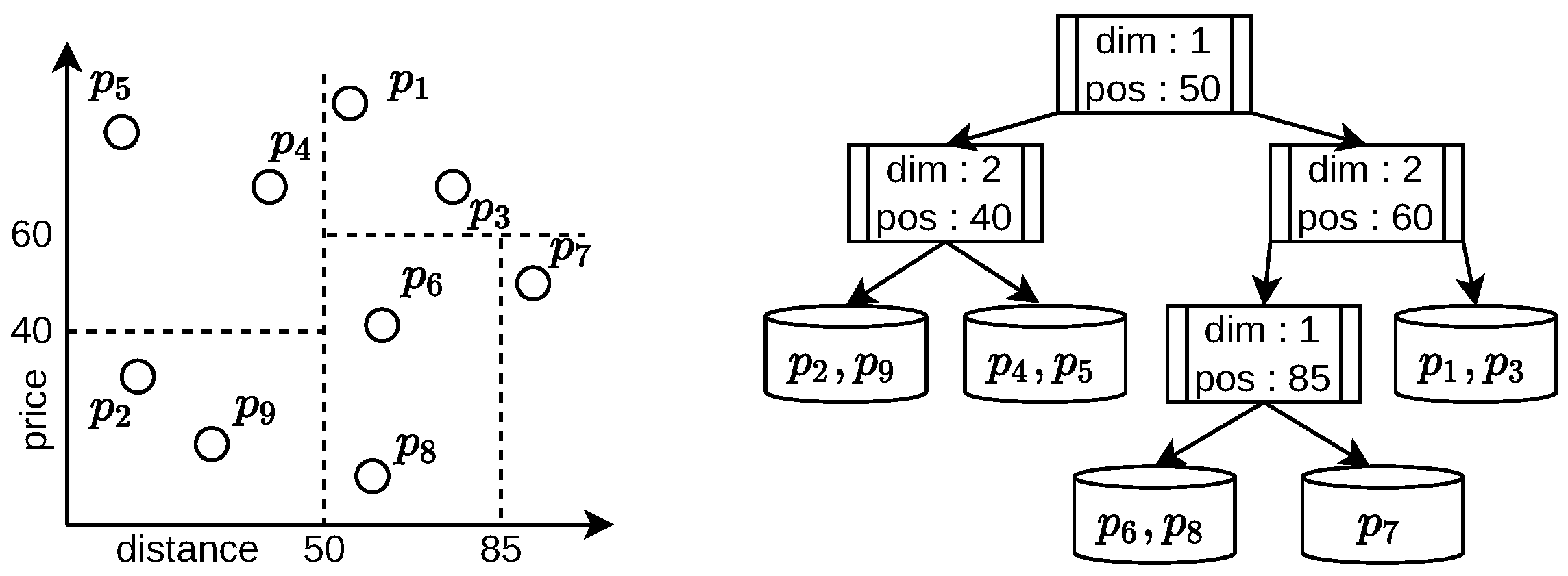
The LSD tree with maximum bucket size and dimension in our running example. Each dashed line represents a dictionary node separating a cuboid into two sub-cuboids. The remaining cuboids represent the bucket nodes. For instance, the root of the LSD tree is a dictionary node that splits the feature vectors at x-position 50 (given we interpret the x and y dimensions as Dimensions 1 and 2), into two sets.
Figure 2.
The LSD tree with maximum bucket size and dimension in our running example. Each dashed line represents a dictionary node separating a cuboid into two sub-cuboids. The remaining cuboids represent the bucket nodes. For instance, the root of the LSD tree is a dictionary node that splits the feature vectors at x-position 50 (given we interpret the x and y dimensions as Dimensions 1 and 2), into two sets.

Figure 3.
Geometric interpretation of Lemma 3 on our running example with . By mirroring across q along the coordinate axis (dotted lines), we obtain the grayish-colored nodes. From each grayish-colored node, we spawn a gray-shaded region in which we know that dominates all points contained in that region. In this example, we obtain that and .

Figure 4.
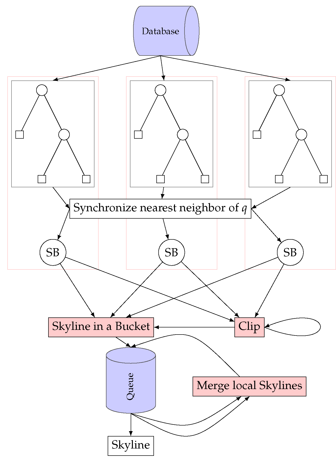
Flow diagram of the parallel Skyline Breaker algorithm ([4], Figure 1). Each thread maintains one LSD tree, which gets populated by the data from a single database source. After reading the data, each thread computes the nearest neighbor of q with respect to the -norm. These neighbors are synchronized across the threads. After that, the Skyline Breaker (SB) algorithm uses these neighbors for clipping the tree. Potential skyline points are put into a queue that is finally merged into the answer set .
Figure 4.
Flow diagram of the parallel Skyline Breaker algorithm ([4], Figure 1). Each thread maintains one LSD tree, which gets populated by the data from a single database source. After reading the data, each thread computes the nearest neighbor of q with respect to the -norm. These neighbors are synchronized across the threads. After that, the Skyline Breaker (SB) algorithm uses these neighbors for clipping the tree. Potential skyline points are put into a queue that is finally merged into the answer set .

Figure 5.
Clipping technique. The rectangles show the buckets of our LSD tree. Given we have a query point q and found a neighbor a of q, we mirror a to all remaining 3 orthants across q, which gives us , , and . We have to scan or have already scanned the light dotted buckets but can omit, thanks to these four points, the cross-hatched buckets. The buckets with stars may still store skyline points, so we have to scan them.

Figure 6.
Experiment varying the size of the input (in millions [M], i.e., ) with four threads. The time (y-axis) is in milliseconds and logarithmic scale. Each row uses a different random distribution of the input values, and each column corresponds to a specific dimension n of the feature vectors. The number of input tuples varies from 100,000 to 700,000 with steps of 100,000 units.

Figure 7.
Experiment varying the number of threads with fixed input size of 700,000 tuples. The time (y-axis) is in milliseconds and logarithmic scale. Each row uses a different random distribution of the input values, and each column corresponds to a specific dimension n of the feature vectors. The number of threads varies from one to four.


Table 1.
Feature vectors of our running example with skyline set (with respect to ) and dynamic skyline set for three different query points , and . The columns show the absolute difference between a query vector and a feature vector in each dimension. We show in the column dom by which vector the vector in the respective row got dominated; here a dash (−) says that this vector is not dominated by any vectors of the input set. Dominated vectors are not part of the skyline set.
| Vector | |||||||
|---|---|---|---|---|---|---|---|
| dom. | dom. | dom. | dom. | ||||
| = | (10, 35) | (15, 35) | (10, 40) | ||||
| = | − | (35, 25) | (30, 25) | (35, 20) | |||
| = | (25, 15) | (30, 15) | (25, 20) | ||||
| = | (5, 15) | − | (0, 15) | − | (5, 20) | − | |
| = | − | (40, 25) | (35, 25) | (40, 30) | |||
| = | (10, 10) | − | (15, 10) | − | (10, 5) | − | |
| = | (45, 5) | − | (50, 5) | − | (45, 0) | − | |
| = | − | (7, 45) | (12, 45) | (7, 40) | |||
| = | − | (20, 35) | (15, 35) | (20, 30) | |||
Disclaimer/Publisher’s Note: The statements, opinions and data contained in all publications are solely those of the individual author(s) and contributor(s) and not of MDPI and/or the editor(s). MDPI and/or the editor(s) disclaim responsibility for any injury to people or property resulting from any ideas, methods, instructions or products referred to in the content. |
© 2023 by the author. Licensee MDPI, Basel, Switzerland. This article is an open access article distributed under the terms and conditions of the Creative Commons Attribution (CC BY) license (https://creativecommons.org/licenses/by/4.0/).
Share and Cite
MDPI and ACS Style
Köppl, D. Dynamic Skyline Computation with LSD Trees. Analytics 2023, 2, 146-162. https://doi.org/10.3390/analytics2010009
AMA Style
Köppl D. Dynamic Skyline Computation with LSD Trees. Analytics. 2023; 2(1):146-162. https://doi.org/10.3390/analytics2010009
Chicago/Turabian StyleKöppl, Dominik. 2023. "Dynamic Skyline Computation with LSD Trees" Analytics 2, no. 1: 146-162. https://doi.org/10.3390/analytics2010009