Proceeding Paper

Further Remarks on Irrational Systems and Their Applications †

by
Adrián-Josué Guel-Cortez
1,*,
César-Fernando Méndez-Barrios
2,
Diego Torres-García
2 and
Liliana Félix
2
1
Centre for Fluid and Complex Systems, Coventry University, Coventry CV1 5FB, UK
2
Faculty of Engineering, Autonomous University of San Luis Potosi, San Luis Potosi 78210, Mexico
*
Author to whom correspondence should be addressed.
Presented at the 5th Mexican Workshop on Fractional Calculus (MWFC), Monterrey, Mexico, 5–7 October 2022.
Comput. Sci. Math. Forum 2022, 4(1), 5; https://doi.org/10.3390/cmsf2022004005
Published: 22 December 2022
(This article belongs to the Proceedings of The 5th Mexican Workshop on Fractional Calculus)

Abstract

:
Irrational Systems (ISs) are transfer functions that include terms with irrational exponents. Since such systems are ubiquitous and can be seen when solving partial differential equations, fractional-order differential equations, or non-linear differential equations; their nature seems to be strongly linked with a low-order description of distributed parameter systems. This makes ISs an appealing option for model-reduction applications and controls. In this work, we review some of the fundamental concepts behind a set of ISs that are of core importance in their stability analysis and control design. Specifically, we introduce the notion of multivalued functions, branch points, time response, and stability regions, as well as some practical applications where these systems can be encountered. The theory is accompanied by some numerical examples or simulations.

1. Introduction

Irrational Systems (ISs) can be found when solving partial differential equations, fractional-order differential equations, or non-linear differential equations [1]. ISs have also been called implicit operators since they often come from solving a second-order polynomial whose solution describes the total impedance of infinite linear lumped-element networks (for further details, see [2]). In addition, fractional behavior or non-exponential decay can also be associated with ISs due to their time-response, often related to special functions such as Bessel or error functions [3]. Hence, ISs’ nature is strongly linked to a low-order description of distributed parameter systems, making ISs an appealing option for control and model-reduction applications.
In the literature, ISs have been applied as mathematical models in different scenarios. For instance, ref. [4] uses fractances in a lumped model of the cardiovascular system, leading to the description of different types of heart anomalous behaviors. In [3,5,6], ISs are introduced to describe robotic formations in the form of tree-like networks and ladder-like networks. Ref. [7] models pipeline-infinite networks that converge to an IS. Similarly, ref. [8] shows an application of ISs to model electrical line transmissions.
When talking about control applications, in our previous work [9], we discuss the stability and control for a type of IS driven by fractional-order controls. Then, in [10], we formalize our analysis and apply the fractional-order controls of the type proportional-integral (PI) and proportional-derivative (PD), including their fragility analysis.
As the conceptualisation and application of ISs to engineering are still under development, in this work, we summarize the fundamental concepts, assumptions, and limits of ISs. The summary aims to briefly explain IS stability analysis and control based on our previous and undergoing investigations. The work is organized as follows: Section 2 defines the fundamental concepts and details the origins of ISs. It also discusses the intrinsic connection between fractional calculus and ISs. Furthermore, it states the fundamental hypothesis when applying ISs in system modeling. Section 3 describes the conditions of stability for ISs. Section 4 briefly explains how to design low-order controllers of the type PD- μ (i.e., fractional-order proportional-derivative controls) for the kind of ISs that the paper focuses on. Section 5 gives some examples of ISs’ control. Finally, Section 6 provides concluding remarks and outlines future work.

2. Preliminaries

Before formally describing the set of ISs that this work will discuss, we need to introduce the following concepts:
Definition 1
(Multivalued function [11,12]). A multivalued function is any complex function F : C C satisfying
F [ z ( r , θ + 2 π ) ] F [ z ( r , θ ) ] ,
where r and θ are the magnitude and argument of the complex variable z C .
Definition 2
(Branch points and branch cuts [13]). The Branch point (BP) or point of accumulation is defined as the point with the smallest magnitude for which a function is multivalued. Another definition would be: a branch point is a point such that the function is discontinuous when going around an arbitrarily small circuit around this point.
It is now easier to understand the following definition of an IS:
Definition 3
(Irrational system). An irrational system is a multi-valued transfer function G ( s ) with one or more terms raised to the power α Q .
In this work, we consider ISs described by
G ( s ) = N ( s ) + P ( s ) D ( s ) + Q ( s ) ,
where N ( s ) = k = 0 m b k s k , D ( s ) = k = 0 n a k s k , a i , b i , a n 0 are arbitrary real numbers, and n m . Moreover, P ( s ) and Q ( s ) are second-order polynomials with positive real coefficients defined as P ( s ) = k = 0 N β k s N and Q ( s ) = k = 0 N γ k s N , respectively.
Clearly, according to Definition 3, the open-loop system (2) and IS with α = 1 2 , and branch points are located at the roots of P ( s ) and Q ( s ) .

Origins and Connection with Fractional Calculus

Irrational transfer functions such as (2) are proven to appear when modeling infinite networks of lumped elements (for a complete description, see [1,7]). The proof of such a statement, omitted here for brevity, requires the following assumptions:
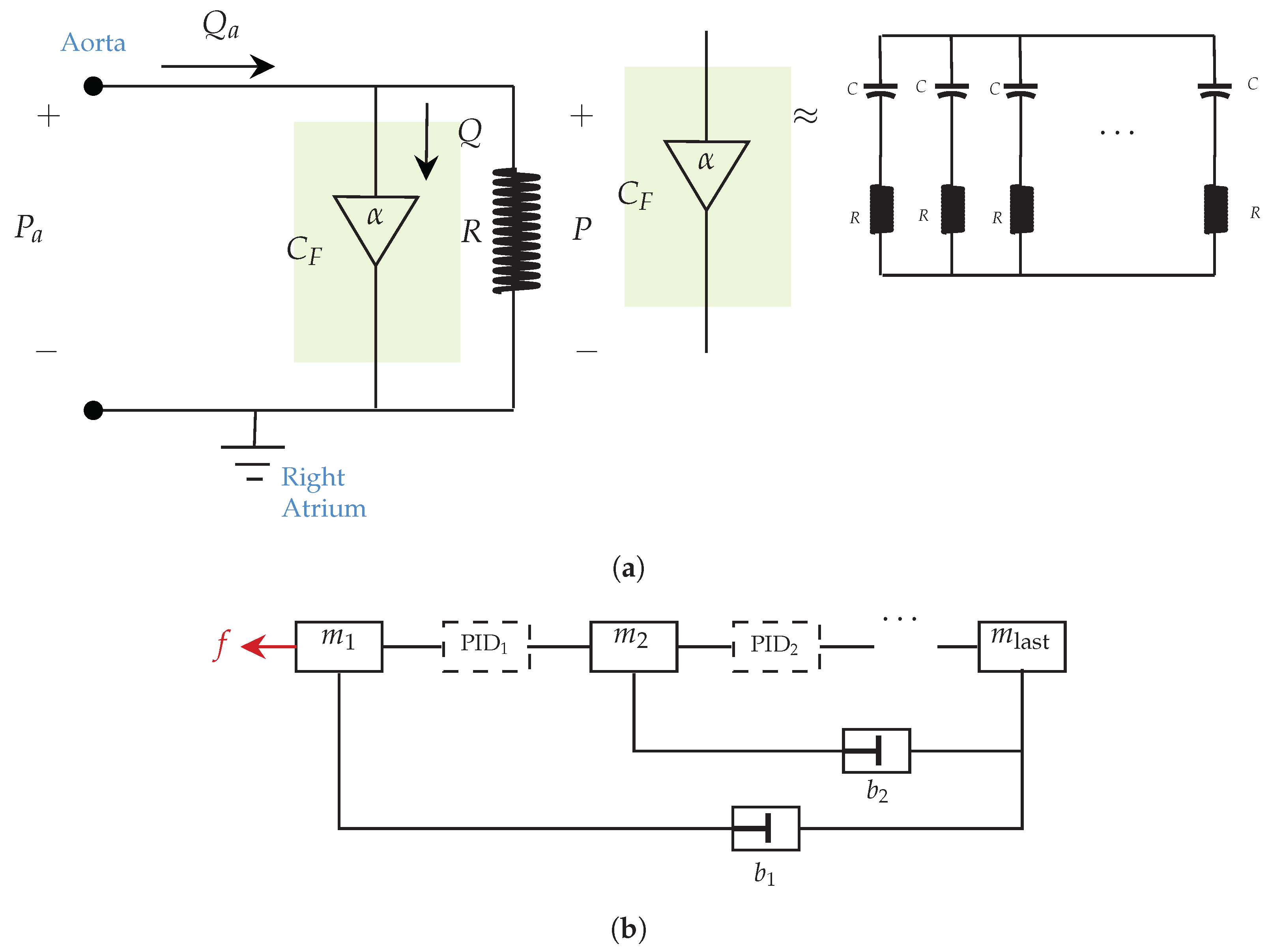
  • The network should contain only linear lumped elements. For instance, viscous dampers, springs, capacitors, or inductors.
  • All initial conditions should be equal to zero.
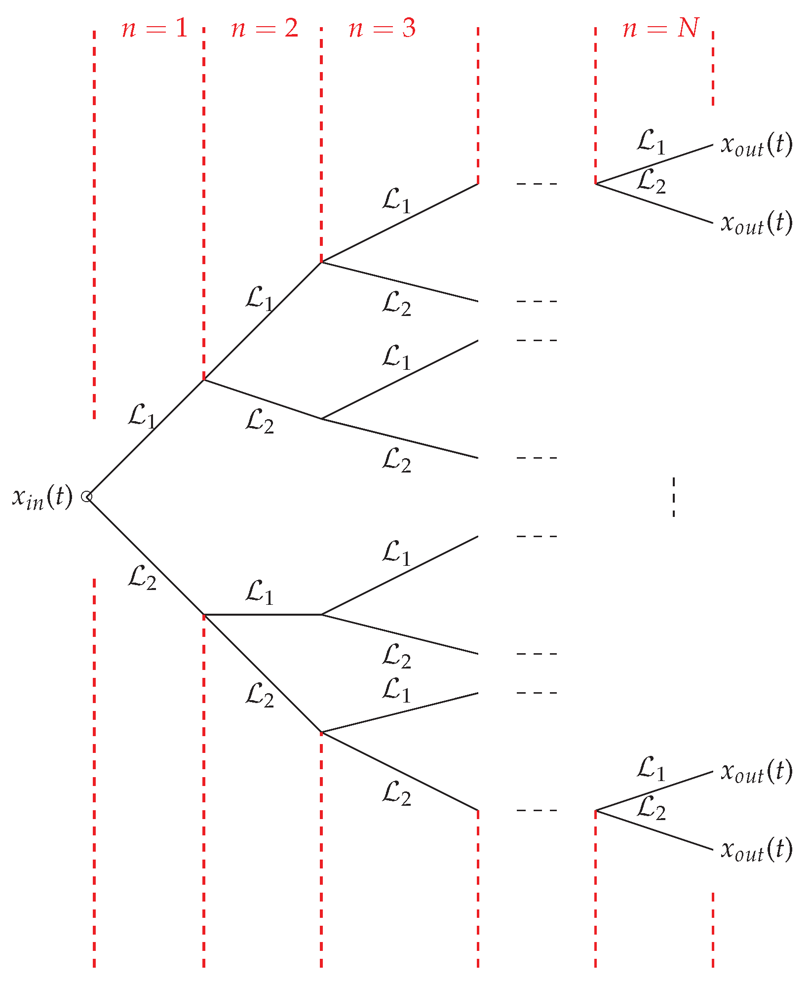
  • Elements in the network should have equal impedance value. For example, the tree-like network shown in Figure 1 contains only two linear operators L 1 and L 2 , which have the same value throughout all the layers of the network.
  • The network is one-dimensional and infinite.
In spite of such necessary conditions, ISs can still be applied in many scenarios, epecially when the following hypotheses are considered:
Hypothesis 1.
The accuracy of 0-dimensional models of complex dynamical systems can increase by adding “networks” as lumped elements in the model.
Hypothesis 2.
ISs can be used as model reductions for large-scale dynamical systems.
The validity of Hypothesis 1 has been proved in scenarios such as the cardiovascular system [4,14] or muscle/joint modeling [15].
On the other hand, Hypothesis 2 has been explored in robot formations and transmission lines (for further details, see [6,16,17,18]). Furthermore, in some cases the ISs description leads to basic fractional-order transfer functions (for instance, see [18]).
For a better understanding of Hypotheses 1 and 2, consider the circuit-like description of the cardiovascular system shown in Figure 2a and the graphical description of a formation of mobile robots in one dimension in Figure 2b. In the case of Figure 2a, we can assume that one of the elements is itself an infinite network of linear elements with an impedance equal to 1 C F α s α (i.e., of fractional-order); then, its mathematical model is given by
0 D t α P a = Q a C F α P a R C F α .
Furthermore, by using the Caputo definition of the fractional derivative operator 0 D t α of order 0 < α < 1 , the time response of system (3) is given by
P a ( t ) = P a ( 0 ) t α 1 E α , α ( 1 R C F α t α ) + 1 C F α 0 t Q a ( t τ ) τ α 1 E α , α ( 1 R C F α τ α ) d τ ,
where E α , α ( z ) is the Mittag–Leffler function of the complex value z [19]. Equation (4) describes the arterial pressure as a power law equation with a diffusive term. Even though this kind of representation implies some physical challenges that have been recently discussed through various works (for instance, see [20,21] and the references therein), it is clear that we can substitute any IS’s impedance instead of a simple lumped element to expand the capabilities of 0-dimensional models, as discussed in Hypothesis 1.
Regarding Hypothesis 2, Figure 2b shows a PID-driven robotic formation in one-dimension (for example, see [22]) where all robots are described as simple mechanical elements. If we regard the network as infinite, the transfer function relating the leader’s position and the last robot in the formation would be an IS [6]. Is this representation a good approximation of the actual transfer function when the number of robots in the network is finite? The answer is still not conclusive and requires further investigation (a preliminary analysis is given in [3]).

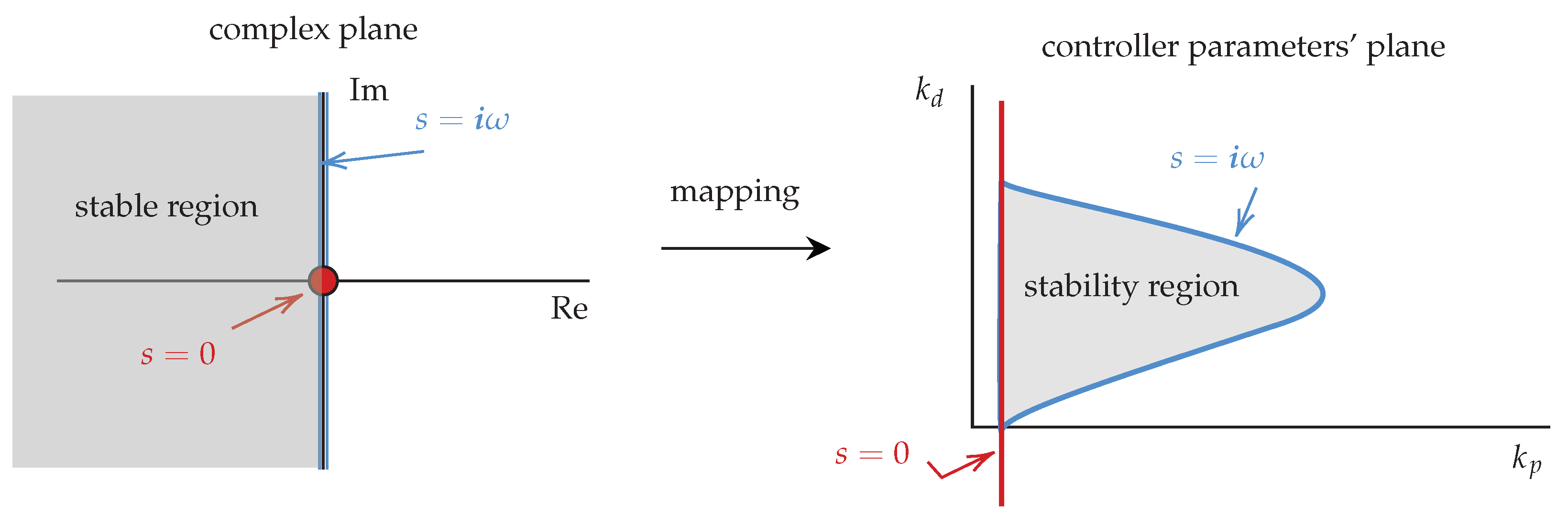
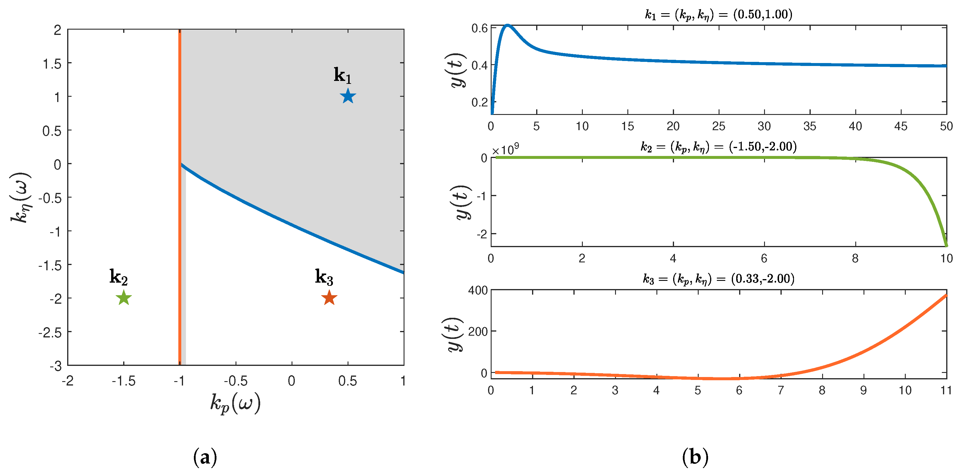
3. Stability Analysis
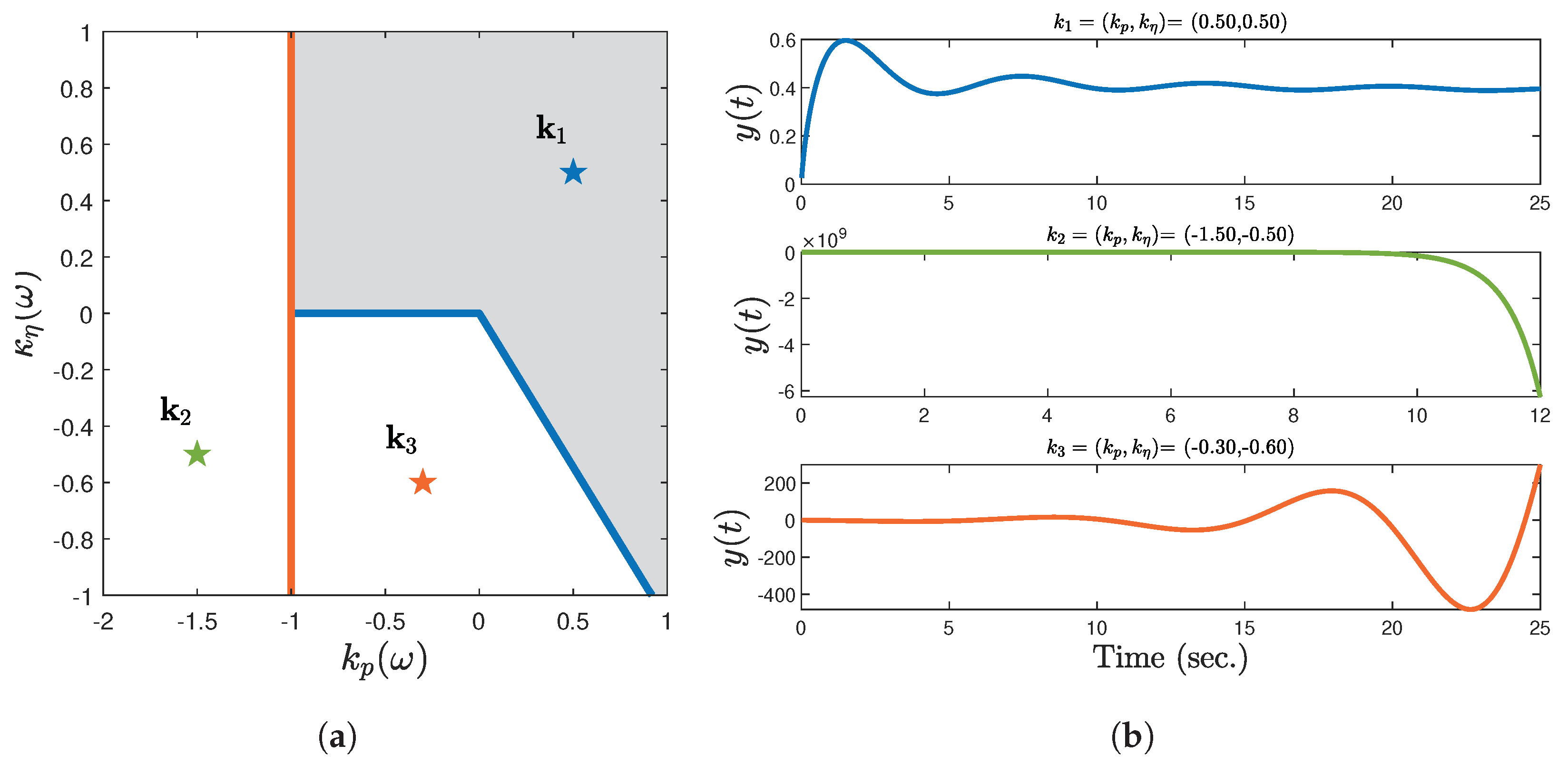
One of the great advantages of ISs mathematical models is that we can easily study their stability if the following Theorem is considered:
Theorem 1
([8]). A given multivalued transfer function is stable if and only if it has no pole in C + and no branch points in C . Here, C + and C stand for the closed right half plane (RHP) and the open RHP of the first Riemann sheet in the complex plane, respectively.
Briefly, Theorem 1 states that the BPs should not be located in the right-hand side of the complex plane to achieve the IS’s stability. To grasp this conclusion, let us consider the following simple examples:
Example 1.
Consider the multivalued transfer function
G ( s ) = 1 s + k ,
where k R . The impulse response of (5) is given by (proof given in Appendix A)
y ( t ) = L 1 1 s + k = e k t π t k > 0 e k t π t k < 0 1 π t k = 0 .
In Example 1, the IS (5) is stable iff k > 0 . Note that as mentioned earlier, the BP is located at the root of the radicand s + k .
Example 2.
Consider the multivalued transfer function
G ( s ) = 1 s 2 + k ,
where k R . The impulse response of (7) is given by (see Appendix B)
y ( t ) = L 1 1 s 2 + k = J 0 ( k t ) k > 0 J 0 ( i k t ) k < 0 1 k = 0 .
Equation (7) is an example where the open-loop IS is stable as the BPs are located in the imaginary-axis and not in the right-hand side of the complex plane.

4. Control Design

PD μ Control

Once the stability conditions for ISs are established, it is possible to design stabilising low-order controllers by following the D-composition method [23]. The following summarizes the procedure, but a complete guide can be found at references [10,24,25].
First, consider a low-order controller, for instance, the fractional-order PD control whose transfer function is well-known to be [9]
C ( s ) = k p + k d s μ .
Then, compute the characteristic polynomial of (2). In this case defined as
Δ ( s ) : = D ( s ) + Q ( s ) + N ( s ) + P ( s ) k p + k d s μ .
Now, substitute the stability boundary of the complex plane s = i ω in the characteristic polynomial and solve for the control gains.
Remark 1.
Note that the substitution of s = i ω requires one to consider the cases ω = 0 , ω and ω 0 separately [25]. In this manner, we create various sets of stability boundaries in the controller’s parameter plane that permit us to enclose a stability region (See Figure 3).

5. Applications

5.1. Control of IS

We now apply the D-composition method to some specific ISs. Note that, in all examples, the time response of the ISs closed-loop is obtained numerically using the inverse numerical Laplace transform proposed in [26]. Furthermore, fixed parameters have been selected randomly as the example’s purpose is to prove the results’ validity.

5.2. Bessel

Consider the Laplace transform of the Bessel function of order zero described as
1 s 2 + 1 .
Therefore, the characteristic function is given by
Δ ( s ) = s 2 + 1 + k p + k d s μ .
Setting μ = 0.3 and solving (12) for k p and k d , we obtain two stability boundaries shown in red and blue in Figure 4a. The red curve corresponds to the case where ω = 0 before solving Δ ( i ω ) = 0 , while the blue corresponds to the case where ω 0 . Figure 4b shows the closed-loop response of a set of controller gains inside and outside of what is found to be the IS’s stability region.

5.3. First Order IS

Another example of an IS that can be controlled by a fractional-order PD control is
3 s + 1 s + 2 s + 1 .
In this case, the characteristic equation is
Δ ( s ) = s + 2 s + 1 + 3 s + 1 .
Likewise, in the previous application we set μ = 0.4 and solved (14) for k p and k d to obtain the stability boundaries shown in Figure 5a. Again, the red curve corresponds to the case where ω = 0 before solving Δ ( i ω ) = 0 , while the blue corresponds to the case where ω 0 . Figure 5b shows the closed-loop response of a set of controller gains inside and outside of what is found to be the IS’s stability region.

6. Conclusions

In this work, we have briefly described the concepts, hypotheses, and assumptions behind the use of ISs. In addition, in our applications, we present the stability analysis and control of ISs. As can be seen by the reader, future work may take various paths, including the design of different low-order controls for ISs, the application of ISs to model other complex phenomena, or the creation of irrational controls that could stabilize ISs whose BPs are in the right-hand side of the complex plane.

Author Contributions

Conceptualization, A.-J.G.-C. and C.-F.M.-B.; methodology, A.-J.G.-C.; software, A.-J.G.-C. and D.T.-G.; validation, A.-J.G.-C., C.-F.M.-B., and D.T.-G.; formal analysis, A.-J.G.-C. and C.-F.M.-B.; investigation, A.-J.G.-C.; resources, A.-J.G.-C. and L.F.; data curation, A.-J.G.-C., D.T.-G., and L.F.; writing—original draft preparation, A.-J.G.-C. and D.T.-G.; writing—review and editing, C.-F.M.-B. and L.F.; visualization, A.-J.G.-C.; supervision, A.-J.G.-C. and C.-F.M.-B.; project administration, A.-J.G.-C. and C.-F.M.-B.; and funding acquisition, L.F. All authors have read and agreed to the published version of the manuscript.

Funding

This research was funded by Faculty of Engineering, Autonomous University of San Luis Potosi grant number POA-AME-IMT2022.

Institutional Review Board Statement

Not applicable.

Informed Consent Statement

Not applicable.

Data Availability Statement

Not applicable.

Conflicts of Interest

The authors declare no conflict of interest.

Abbreviations

The following abbreviations are used in this manuscript:
ISIrrational system
PDProportional derivative
PIProportional integral
BPBranch point
PIDProportional integral derivative

Appendix A. Example 1

To compute the time-response of the multivalued transfer function in (5), we consider the following definition of the inverse Laplace transform:
y ( t ) = L 1 1 s + k = 1 2 i π c c + G ( s ) e s t d s .
To solve (A1), let the contour C be defined as the sum of C i , i [ 1 , 6 ] , as shown in Figure A1. Note that the election of the integration path should be one which avoids branch points, namely, point k in this scenario.
Figure A1. Integration path of Example 1.
Csmf 04 00005 g0a1
According to the residue theorem
C G ( s ) e s t d s = 0 .
Then, we can express (A1) as
B r G ( s ) e s t d s = i = 1 5 C i G ( s ) e s t d s .
Observe that, for R
C 1 = C 5 = 0 ,
and, on the other hand, for ρ 0 we have
C 3 = 0 .
Thus, it suffices to compute the integration along C 2 and C 4 to obtain y ( t ) . In order to perform such an operation, consider the parameterisation s + k = r , which in polar form can be rewritten as r e ± i π , where the positive sign corresponds to C 2 and the negative sign corresponds to C 4 . This permits us describe the path r ( k + ρ , ) , with δ , ρ 0 , i.e.,
C 2 + C 4 = ρ e ( r + k ) t e i π r e i π / 2 d r + ρ e ( r + k ) t e i π r e i π / 2 d r ,
since ρ 0
C 2 + C 4 = ( e i π + e i π ) 0 e ( r + k ) t r d r = 2 i sin ( π / 2 ) e k t 0 e r t r d r = 2 i sin ( π / 2 ) e k t t 1 / 2 Γ ( 1 / 2 ) .
Now, as we know that
Γ ( x ) Γ ( 1 x ) = π sin ( π x ) ,
with x = 1 / 2 , from (A1) we have,
L 1 1 s + k = e k t t π .
This finishes the proof of statement (6).

Appendix B. Example 2

Following the ideas used to find the inverse Laplace Transform of 1 s + k shown in Appendix A, we now perform the time-response of (7) (given in Equation (8)) by computing
y ( t ) = L 1 1 s 2 + k = 1 2 i π c c + G ( s ) e s t d s .
Observe that for k > 0 , we have a complex conjugate branch point, while for k < 0 we have two real points. Under these observations, we consider two different integration paths, shown in Figure A2, where Figure A2a and Figure A2b correspond to the case of k negative and positive, respectively.
Figure A2. Integration path of Example 2. (a) k < 0 . (b) k > 0 .
Csmf 04 00005 g0a2
We first consider the case k < 0 ; thus, we shall consider the path shown in Figure A2a and create a path such that
C G ( s ) e s t d s = 0 .
Under the assumption that ρ 0 ,
C 1 + C 2 = 0 .
Now, C 3 and C 4 s vary from k ρ to k + ρ , and then we have
C 2 + C 3 e s t s 2 k = i k + ρ k ρ e s t k s 2 + i k ρ k + ρ e s t k s 2 = 2 i k + ρ k ρ e s t k s 2 .
Since ρ 0 ,
y ( t ) = 1 2 π i B r G ( s ) e s t d s = 1 π k k e s t k s 2 .
Then, making s = a cos ( u ) , the integral becomes
1 π 0 π e k t cos ( u ) d u = I 0 ( k t ) .
We can express the modified first Bessel function in terms of the first Bessel function if π < arg ( k t ) π 2 :
J α ( i k t ) = e α π 2 I α ( k t )
with α = 0 :
J 0 ( i k t ) = I 0 ( k t ) .
Now, we consider the case where k > 0 . The inverse Laplace transform of G ( s ) can be written in two different forms (see for instance [27]):
y ( t ) = 2 π k sin ( s t ) 1 s 2 k d s ,
y ( t ) = 2 π 0 k cos ( s t ) 1 k s 2 d s .
The first Bessel function is given as
J 0 ( x ) = 1 π 0 π cos ( x sin ( τ ) ) d τ .
Thus, by taking s = k sin ( θ ) in (), with θ ( 0 , π 2 ) we have
y ( t ) = 2 π 0 π 2 cos ( k t sin ( θ ) ) d θ = 2 π π 2 J 0 ( k t ) .

References

  1. Guel-Cortez, A.J. Modeling and Control of Fractional-Order Systems. The Linear Systems Case. Ph.D. Thesis, CIEP-UASLP, San Luis, Mexico, 2018. [Google Scholar]
  2. Sen, M.; Hollkamp, J.P.; Semperlotti, F.; Goodwine, B. Implicit and fractional-derivative operators in infinite networks of integer-order components. Chaos Solitons Fractals 2018, 114, 186–192. [Google Scholar] [CrossRef]
  3. Guel-Cortez, A.J.; Sen, M.; Goodwine, B. Closed form time response of an infinite tree of mechanical components described by an irrational transfer function. In Proceedings of the 2019 American Control Conference (ACC), Philadelphia, PA, USA, 10–12 July 2019; pp. 5828–5833. [Google Scholar]
  4. Guel-Cortez, A.J.; Kim, E. A Fractional-Order Model of the Cardiac Function. In Proceedings of the 13th Chaotic Modeling and Simulation International Conference, Florence, Italy, 9–12 June 2020; Springer: Berlin/Heidelberg, Germany, 2020; pp. 273–285. [Google Scholar]
  5. Leyden, K.; Sen, M.; Goodwine, B. Large and infinite mass–spring–damper networks. J. Dyn. Syst. Meas. Control 2019, 141, 061005. [Google Scholar] [CrossRef]
  6. Ni, X.; Goodwine, B. Frequency Response and Transfer Functions of Large Self-similar Networks. arXiv 2020, arXiv:2010.11015. [Google Scholar] [CrossRef]
  7. Mayes, J.; Sen, M. Approximation of potential-driven flow dynamics in large-scale self-similar tree networks. Proc. R. Soc. A Math. Phys. Eng. Sci. 2011, 467, 2810–2824. [Google Scholar] [CrossRef] [Green Version]
  8. Merrikh-Bayat, F.; Karimi-Ghartemani, M. On the essential instabilities caused by fractional-order transfer functions. Math. Probl. Eng. 2008, 2008, 419046. [Google Scholar] [CrossRef]
  9. Guel-Cortez, A.J.; Sen, M.; Goodwine, B. Fractional- PDμ Controllers for Irrational Systems. In Proceedings of the 2019 International Conference on Control, Decision and Information Technologies, Paris, France, 23–26 April 2019. [Google Scholar]
  10. Guel-Cortez, A.J.; Méndez-Barrios, C.F.; Kim, E.j.; Sen, M. Fractional-order controllers for irrational systems. IET Control Theory Appl. 2021, 15, 965–977. [Google Scholar] [CrossRef]
  11. Cohen, H. Complex Analysis with Applications in Science and Engineering; Springer Science & Business Media: Berlin/Heidelberg, Germany, 2007. [Google Scholar]
  12. Harvey, C. Conformal mapping on Riemann Surfaces; Dover Publications, Inc.: New York, NY, USA, 1980. [Google Scholar]
  13. Needham, T. Complex Visual Analysis; Oxford University Press, Inc.: New York, NY, USA, 1997. [Google Scholar]
  14. Capoccia, M. Development and characterization of the arterial W indkessel and its role during left ventricular assist device assistance. Artif. Organs 2015, 39, E138–E153. [Google Scholar] [CrossRef] [PubMed] [Green Version]
  15. Piovesan, D.; Pierobon, A.; DiZio, P.; Lackner, J.R. Measuring multi-joint stiffness during single movements: Numerical validation of a novel time-frequency approach. PLoS ONE 2012, 7, e33086. [Google Scholar] [CrossRef] [Green Version]
  16. Ni, X.; Goodwine, B. Frequency Response of Transmission Lines with Unevenly Distributed Properties with Application to Railway Safety Monitoring. arXiv 2020, arXiv:2012.09247. [Google Scholar]
  17. Leyden, K.; Goodwine, B. Using fractional-order differential equations for health monitoring of a system of cooperating robots. In Proceedings of the 2016 IEEE International Conference on Robotics and Automation (ICRA), Stockholm, Sweden, 16–21 May 2016; pp. 366–371. [Google Scholar]
  18. Leyden, K.; Sen, M.; Goodwine, B. Models from an implicit operator describing a large mass-spring-damper network. IFAC-PapersOnLine 2018, 51, 831–836. [Google Scholar] [CrossRef]
  19. Shukla, A.; Prajapati, J. On a generalization of Mittag-Leffler function and its properties. J. Math. Anal. Appl. 2007, 336, 797–811. [Google Scholar] [CrossRef]
  20. Sabatier, J.; Farges, C.; Tartaglione, V. Some alternative solutions to fractional models for modelling power law type long memory behaviors. Mathematics 2020, 8, 196. [Google Scholar] [CrossRef] [Green Version]
  21. Sabatier, J. Some Proposals for a Renewal in the Field of Fractional behavior Analysis and Modelling. In Proceedings of the International Conference on Fractional Differentiation and its Applications (ICFDA’21); Springer: Berlin/Heidelberg, Germany, 2022; pp. 1–25. [Google Scholar]
  22. Ramos-Avila, D.; Rodrıguez, C.; Hernández-Carrillo, J.; Guel-Cortez, A.; Sen, M.; Méndez-Barrios, C.; González-Galván, E.; Goodwine, B. Experiments with PD-controlled robots in ring formation. In Proceedings of the XXI Congreso Mexicano de Robótica–COMRob, Ciudad de Manzanillo, Colima, Mexico, 13–15 November 2019. [Google Scholar]
  23. Gryazina, E.N. The D-decomposition theory. Autom. Remote Control 2004, 65, 1872–1884. [Google Scholar] [CrossRef]
  24. Hernández-Díez, J.E.; Méndez-Barrios, C.F.; Mondié, S.; Niculescu, S.I.; González-Galván, E.J. Proportional-delayed controllers design for LTI-systems: A geometric approach. Int. J. Control 2018, 91, 907–925. [Google Scholar] [CrossRef]
  25. Barrios, C.F.M. Low-Order Controllers for Time-Delay Systems: An Analytical Approach. Ph.D. Thesis, Université Paris Sud-Paris XI, Bures-sur-Yvette, France, 2011. [Google Scholar]
  26. Abate, J.; Whitt, W. A unified framework for numerically inverting Laplace transforms. INFORMS J. Comput. 2006, 18, 408–421. [Google Scholar] [CrossRef]
  27. Moslehi, L.; Ansari, A. Some remarks on inverse Laplace transforms involving conjugate branch points with applications. UPB Sci. Bull. Ser. A-Appl. Math. Phys. 2016, 78, 107–118. [Google Scholar]
Figure 1. Tree-like network of N layers that can be described by an ISs transfer function. In the network, it is necessary to have L 1 and L 2 to be linear operators. Note that all end-points x o u t are in the same position. The movement is in one-dimension.
Csmf 04 00005 g001
Figure 2. Examples of the application of Hypothesis 1 and 2 in realistic scenarios. (a) Model reduction of the cardiovascular system by an electrical system using a fractance. (b) Ladder network description of mobile robots described by mechanical elements and driven by PID controls [6].
Csmf 04 00005 g002
Figure 3. Example of the D-composition method. The method maps the complex plane stability region to the controller parameters’ plane. In this case, the plane has not stability boundary at s .
Csmf 04 00005 g003
Figure 4. Stability analysis of system (11). (a) Stability region (gray) of the closed-loop system with μ = 0.3 . (b) Time response for control gains inside different regions on the parameter’s plane.
Csmf 04 00005 g004
Figure 5. Stability analysis of system (13). (a) Stability region (gray) of the closed-loop system with μ = 0.4 . (b) Time response for control gains inside different regions on the parameter’s plane.
Csmf 04 00005 g005
Disclaimer/Publisher’s Note: The statements, opinions and data contained in all publications are solely those of the individual author(s) and contributor(s) and not of MDPI and/or the editor(s). MDPI and/or the editor(s) disclaim responsibility for any injury to people or property resulting from any ideas, methods, instructions or products referred to in the content.

