
Fractional Approach to the Study of Damped Traveling Disturbances in a Vibrating Medium †

Tecnológico de Monterrey, School of Engineering and Sciences, Atizapán de Zaragoza 52926, Mexico
†
Presented at the 5th Mexican Workshop on Fractional Calculus (MWFC), Monterrey, Mexico, 5–7 October 2022.
†
Presented at the 5th Mexican Workshop on Fractional Calculus (MWFC), Monterrey, Mexico, 5–7 October 2022.
Comput. Sci. Math. Forum 2022, 4(1), 1; https://doi.org/10.3390/cmsf2022004001
Published: 22 November 2022
(This article belongs to the Proceedings of The 5th Mexican Workshop on Fractional Calculus)
Abstract
:The Cauchy problem of a time–space fractional partial differential equation which has as a particular case the damped wave equation is solved for the Dirac delta initial condition. The solution is obtained in terms of H-Fox functions and models the travel of a disturbance in a vibrating medium.
1. Introduction
In previous works [1,2,3], the fractional space–time partial linear differential equation has been solved. In such an expression, indicates the time fractional derivative in the sense that Caputo (see Ref. [4]), represents the space fractional operator in the sense of Riesz (see Ref. [5]) and is a constant such that , where and stand for the units of length and time, respectively. This equation includes as particular cases the heat equation [6] for , for which , where k stands for the thermometric conductivity, and the wave equation [7,8,9,10], for , for which , where v represents the velocity of propagation of the wave. The Cauchy problem of such an equation with the Dirac delta initial condition is solved by means of Laplace and Fourier methods in Refs. [1,2,3]. In Ref. [1], the equation was solved in terms of generalized Wright functions [11]. The solution has different representations depending on which of the three cases , or is fulfilled. In Ref. [2], a unified representation of the solution was obtained for all possible combinations of and by solving the problem in terms of H-Fox functions. Furthermore, in Ref. [2], a Gaussian initial condition was also considered, leading to a series of H-Fox functions as a solution, where, in the appropriate limit, the solution for the Dirac delta initial condition is recovered. In Ref. [3], attention is paid to the particular case . The solution is obtained in terms of the well-known sine and cosine trigonometric functions. In the first two cases (Refs. [1,2]), the solution depends on the parameters and . Its solution enables on to recover the heat and wave equation solutions for and , respectively. In the last case, (Ref. [3]), the main results depend on and enable one to recover the wave equation solution for . In addition, the integro-differential equations of integer order arise as particular cases of the mentioned equation: the first is obtained for (see Refs. [1,2]) and the second for (see Ref. [2]). The last is introduced in Ref. [2] as a complementary equation, a broader analysis of an such equation is made in Ref. [12].
In a recent work [13], the Cauchy problem of the more general fractional differential expression () that includes as a particular case the Klein–Gordon equation [14] (for its classical applications see, e.g., [15]), is solved in terms of a series of H-Fox functions. The solution is reduced to that of the equation in the limit .
Numerical techniques to solve space–time fractional differential equations were proposed in Refs. [16,17,18,19]. In [16], they aimed to solve the equations of the wave type and in Ref. [17], they aimed to solve the equations of the telegraph form, in both cases with constant coefficients. In Ref. [18], they aimed to solve equations of the Klein–Gordon-type and in Ref. [19], of a more general form, in these two last cases with variable coefficients.
Motivated by those previous works, we consider now the study of a fractional differential equation that includes as a limit case the damped wave equation. Such an equation has the form with . This work is addressed to solve the Cauchy problem of such a fractional differential equation for Dirac delta initial condition.
2. Problem Formulation
Let us consider the one-dimensional damped wave equation
In Equation (1), represents the damping parameter and the constant v the velocity of the damped wave. By replacing the time derivative operators and in Equation (1) with the Caputo fractional derivative operators and , respectively, (see its definition in Appendix A). We obtain the equation
In Equation (2), and the constant fulfills .
A more general expression of Equation (2) can be obtained by replacing the space-derivative operator in Equation (2) with the Riesz fractional operator (see its definition in Appendix A). We arrive at the expression
In Equation (3), and the constant fulfills . Additionally, and .
Let us consider a fractional -order differential equation with , derivatives defined in the sense of Caputo and solution . The Caputo fractional derivative is reduced to the first and second derivative operators for and , respectively; this permits the equation to transit from a first-order differential equation for to a second-order one for . For , this equation requires two initial conditions to have a completely determined solution. For , the equation requires one initial condition for such purposes. To obtain a solution that permits to transit between the solution to the fractional differential equation for to that of through the parameter , we may impose the initial condition for . Taking into account the last considerations, we may impose the following initial conditions into Equation (3)
3. Solution of the Problem
The Laplace transform of Equation (3) is
In the above equation, . The Fourier transform of Equation (5) is
where and . The algebraic expression (6) is solved by
To obtain the solution , we first recover by taking the inverse Fourier transform of . From the definition of inverse Fourier transform, we have
Setting the initial condition into Equation (8) gives
In Ref. [20], the integral in Equation (9) was calculated (as can also be seen in Ref. [2]), and the result leads to the following expression for
where is the H-Fox function [21,22] (as can also be seen in Appendix A). The inverse Laplace transform of is calculated in the Appendix B and gives the solution as follows
where
4. Discussion of Results
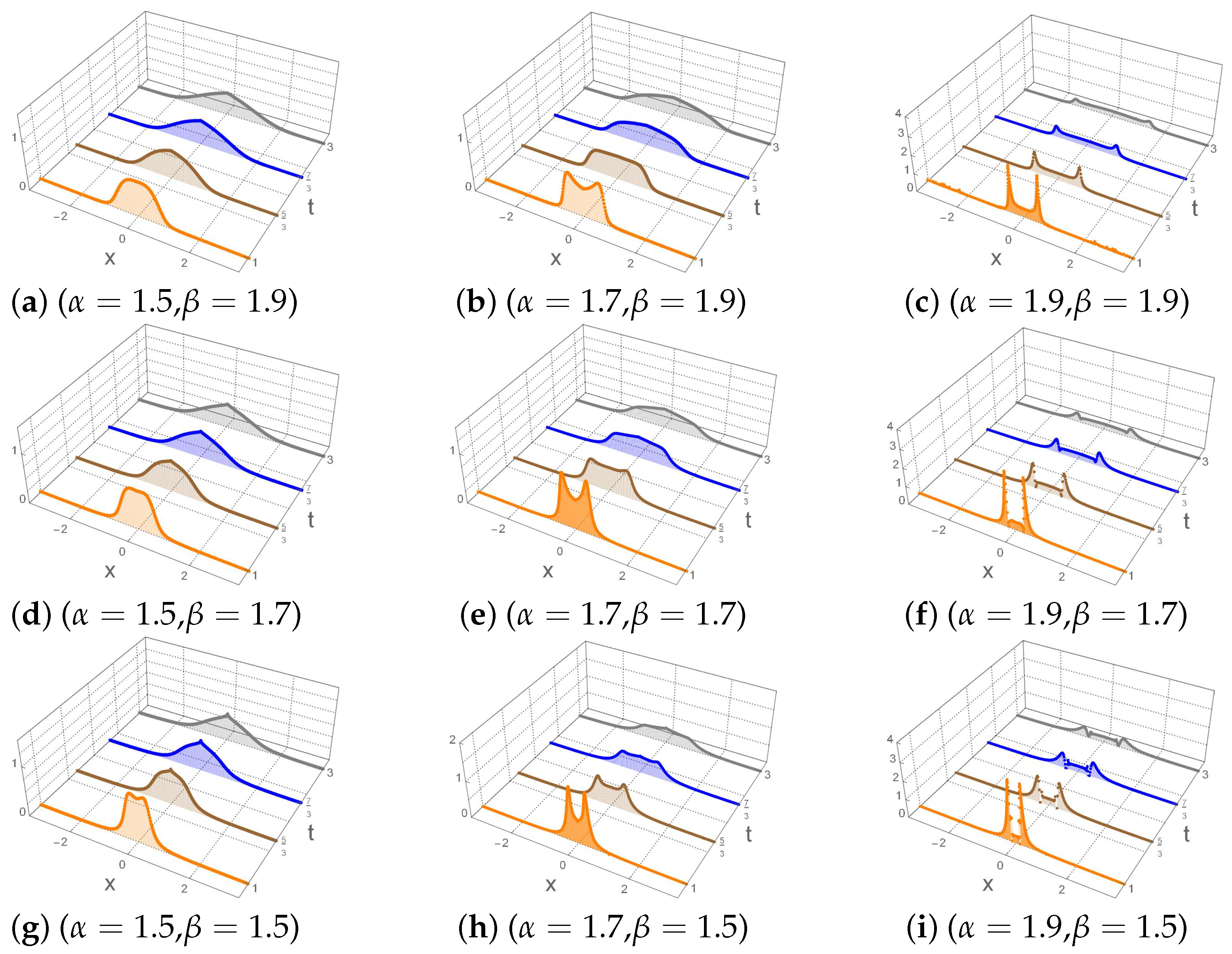
In Figure 1, the graphic representation of the solution is depicted in Equations (11) and (12) for some combinations of . According to the graphics contained in the panel, the solution to Equation (3) can be studied in terms of a disturbance propagating in a vibrating medium. In all the cases presented herein, a mixture of diffusive and wave-like behavior can be observed in the traveling disturbances. As becomes smaller, the diffusive behavior becomes more predominant. As approaches 2, the wave-like behavior is predominant over the diffusive one and the effects of the reduction in the parameter become notorious, as can be observed in the third column with the change in the shape in the center of the traveling disturbances, in contrast to the first and second columns where such changes are not evident. Such a phenomenon may be associated with the presence of jump processes (as can be seen in [23,24,25]) into the traveling disturbance; as is reduced, its effects become more significant.
5. Conclusions
The Cauchy problem for a fractional differential equation with the damped wave equation as a particular case was solved with the Dirac delta initial condition, and its solution was obtained in terms of series of H-Fox functions. According to the graphic representation of the solution, the fractional differential equation models traveling disturbances, where a mixture of wave-like and diffusive behavior is observed. Future work is addressed to the study of a fractional differential equation with the telegrapher equation as a particular case. Such an equation also contains the fractional expressions and as limit cases, which are the second object of study in this work. Work in this direction is in progress and will be reported elsewhere.
Funding
This research has been funded by Consejo Nacional de Ciencia y Tecnología (CONACYT), Mexico, Grant Number A1-S-24569.
Institutional Review Board Statement
Not applicable.
Informed Consent Statement
Not applicable.
Data Availability Statement
Not applicable.
Acknowledgments
The author is grateful to O. Rosas-Ortiz and L.M. Nieto for useful comments.
Conflicts of Interest
The author declares no conflict of interest.
Appendix A. Some Useful Definitions
Let , and . The -order Caputo’s fractional derivative with respect to t of a function f is defined as
Let . The -order Riesz fractional derivative with respect to x of a function f is defined as
where is the Fourier transform of the function f.
The Mellin-Barnes integral of a function f is defined as follows
Let such that and , and (). The H-Fox function is defined via the next Mellin–Barnes integral
The path of integration L separates the poles of to the left and the poles of to the right of L.
Appendix B. Derivation of Expressions (11) and (12)
According to the definition of the H-Fox function provided in (A4), one can express the Equation (10) in its Mellin–Barnes representation as follows
where
The inverse Laplace transform operator acts on the complex variable s, then can be expressed as follows
The series expansion
together with the inverse Laplace transform formula
leads to
From the definition of the H-function, one may write the expression (A12) as follows
References
- Gorenflo, R.; Iskenderov, A.; Luchko, Y. Mapping between solutions of fractional diffusion wave equations. Fract. Calc. Appl. Anal. 2000, 3, 75. [Google Scholar]
- Olivar-Romero, F.; Rosas-Ortiz, O. Transition from the Wave Equation to Either the Heat or the Transport Equations through Fractional Differential Expressions. Symmetry 2018, 10, 524. [Google Scholar] [CrossRef] [Green Version]
- Luchko, Y.J. Fractional wave equation and damped waves. Math. Phys. 2013, 54, 031505. [Google Scholar] [CrossRef] [Green Version]
- Podlubny, I. Fractional Differential Equations; Academic Press: London, UK, 1999. [Google Scholar]
- Umarov, S. Introduction to Fractional and Pseudo-Differential Equations with Singular Symbols; Springer: Basel, Switzerland, 2015. [Google Scholar]
- Widder, D.V. The Heat Equation; Academic Press: New York, NY, USA, 1975. [Google Scholar]
- Tikhonov, A.N.; Samarskii, A.A. Equations of Mathematical Physics; Pergamon Press: New York, NY, USA, 1963. [Google Scholar]
- Gustafson, K.E. Introduction to Partial Differential Equations and Hilbert Space Methods; Dover: New York, NY, USA, 1999. [Google Scholar]
- Duffy, D.G. Green’s Functions with Applications; CRC Press: Boca Raton, FL, USA, 2015. [Google Scholar]
- Borthwick, D. Introduction to Partial Differential Equations; Springer: Basel, Switzerland, 2018. [Google Scholar]
- Luchko, Y. The Wright function and its applications. In Handbook of Fractional Calculus with Applications. Volume 1: Basic Theory; De Gruyte: Berlin, Germany; Boston, MA, USA, 2019; Chapter 10; pp. 241–268. [Google Scholar]
- Olivar-Romero, F.; Rosas-Ortiz, O. An integro-differential Equation of the Fractional Form: Cauchy Problem and Solution. In Integrability, Supersymmetry and Coherent States; A Volume in Honour of Professor Véronique Hussin, CRM Series in Mathematical Physics; Kuru, S., Negro, J., Nieto, L.M., Eds.; Springer: Berlin, Germany, 2019; Chapter 18; pp. 387–393. [Google Scholar]
- Olivar-Romero, F. Fractional Approach to the Study of Some Partial Differential and Integro-Differential Equations. J. Phys. Conf. Ser. 2022. accepted. [Google Scholar]
- Srednicki, M. Quantum Field Theory; Cambridge University Press: Cambridge, UK, 2007. [Google Scholar]
- Gravel, P.; Gauthier, C. Classical applications of the Klein-Gordon equation. Am. J. Phys. 2011, 79, 447. [Google Scholar] [CrossRef]
- Bansu, H.; Kumar, S. Meshless method for the numerical solution of space and time fractional wave equation. In Proceedings of the International Workshop Numerical Solution of Fractional Differential Equations and Applications, Sozopol, Bulgaria, 8–13 June 2020; pp. 11–14. [Google Scholar]
- Bansu, H.; Kumar, S. Numerical Solution of Space and Time Fractional Telegraph Equation: A Meshless Approach. Int. J. Nonlinear Sci. Num. Simul. 2019, 20, 325. [Google Scholar] [CrossRef]
- Bansu, H.; Kumar, S. Numerical Solution of Space-Time Fractional Klein-Gordon Equation by Radial Basis Functions and Chebyshev Polynomials. Int. J. Appl. Comput. Math. 2021, 7, 201. [Google Scholar] [CrossRef]
- Kumar, S.; Piret, C. Numerical solution of space-time fractional PDEs using RBF-QR and Chebyshev polynomials. Appl. Numer. Math. 2019, 143, 300. [Google Scholar] [CrossRef]
- Capelas de Oliveira, E.; Costa, F.; Vaz, J. The fractional Schrödinger equation for delta potentials. J. Math. Phys. 2010, 51, 123517. [Google Scholar] [CrossRef] [Green Version]
- Kilbas, A.A. H-Transforms: Theory and Applications; CRC Press: New York, NY, USA, 2004. [Google Scholar]
- Mathai, A.M.; Saxena, R.K.; Haubold, H.J. The H-Function; Springer: New York, NY, USA, 2010. [Google Scholar]
- Saichev, A.; Zazlavsk, G. Fractional kinetic equations: Solutions and applications. Chaos 1997, 7, 753. [Google Scholar] [CrossRef] [PubMed] [Green Version]
- Gorenflo, E.; Mainardi, F. Random walk models for space-fractional diffusion processes. Fract. Calc. Appl. Anal. 1998, 1, 167. [Google Scholar]
- Gorenflo, R.; Mainardi, F. Approximation to Lévy-Feller diffusion by random walk. Z. Anal. Anwend. 1999, 18, 231. [Google Scholar] [CrossRef]

Publisher’s Note: MDPI stays neutral with regard to jurisdictional claims in published maps and institutional affiliations. |
© 2022 by the author. Licensee MDPI, Basel, Switzerland. This article is an open access article distributed under the terms and conditions of the Creative Commons Attribution (CC BY) license (https://creativecommons.org/licenses/by/4.0/).
Share and Cite
MDPI and ACS Style
Olivar-Romero, F. Fractional Approach to the Study of Damped Traveling Disturbances in a Vibrating Medium. Comput. Sci. Math. Forum 2022, 4, 1. https://doi.org/10.3390/cmsf2022004001
AMA Style
Olivar-Romero F. Fractional Approach to the Study of Damped Traveling Disturbances in a Vibrating Medium. Computer Sciences & Mathematics Forum. 2022; 4(1):1. https://doi.org/10.3390/cmsf2022004001
Chicago/Turabian StyleOlivar-Romero, Fernando. 2022. "Fractional Approach to the Study of Damped Traveling Disturbances in a Vibrating Medium" Computer Sciences & Mathematics Forum 4, no. 1: 1. https://doi.org/10.3390/cmsf2022004001