DAP-SDD: Distribution-Aware Pseudo Labeling for Small Defect Detection ^†

Abstract

Detecting defects, especially when they are small in the early manufacturing stages, is critical to achieving a high yield in industrial applications. While numerous modern deep learning models can improve detection performance, they become less effective in detecting small defects in practical applications due to the scarcity of labeled data and significant class imbalance in multiple dimensions. In this work, we propose a distribution-aware pseudo labeling method (DAP-SDD) to detect small defects accurately while using limited labeled data effectively. Specifically, we apply bootstrapping on limited labeled data and then utilize the approximated label distribution to guide pseudo label propagation. Moreover, we propose to use the t-distribution confidence interval for threshold setting to generate more pseudo labels with high confidence. DAP-SDD also incorporates data augmentation to enhance the model’s performance and robustness. We conduct extensive experiments on various datasets to validate the proposed method. Our evaluation results show that, overall, our proposed method requires less than 10% of labeled data to achieve comparable results of using a fully-labeled (100%) dataset and outperforms the state-of-the-art methods. For a dataset of wafer images, our proposed model can achieve above 0.93 of AP (average precision) with only four labeled images (i.e., 2% of labeled data).

1. Introduction

In the semiconductor industry, detecting small defects at the early stages of manufacturing is crucial for improving yield and saving costs. For example, as wafers are processed in batches or lots, malfunctioning tools or suboptimal operations may result in whole batches of wafers suffering mass yield loss or even being discarded [1,2]. If we can detect anomalies early, tool issues or operation problems can be fixed quickly before more batches of wafers travel through malfunctioning tools or undergo unnecessary value-adding manufacturing processes. Small defects on wafer images usually indicate early-phase tool malfunctions or improper operations. However, due to the high variance of working conditions (e.g., position, orientation, illumination) and complex calibration procedures [2], traditional inspection tools lack the flexibility to detect various defects and suffer from poor detection performance, especially for small and dim defects.

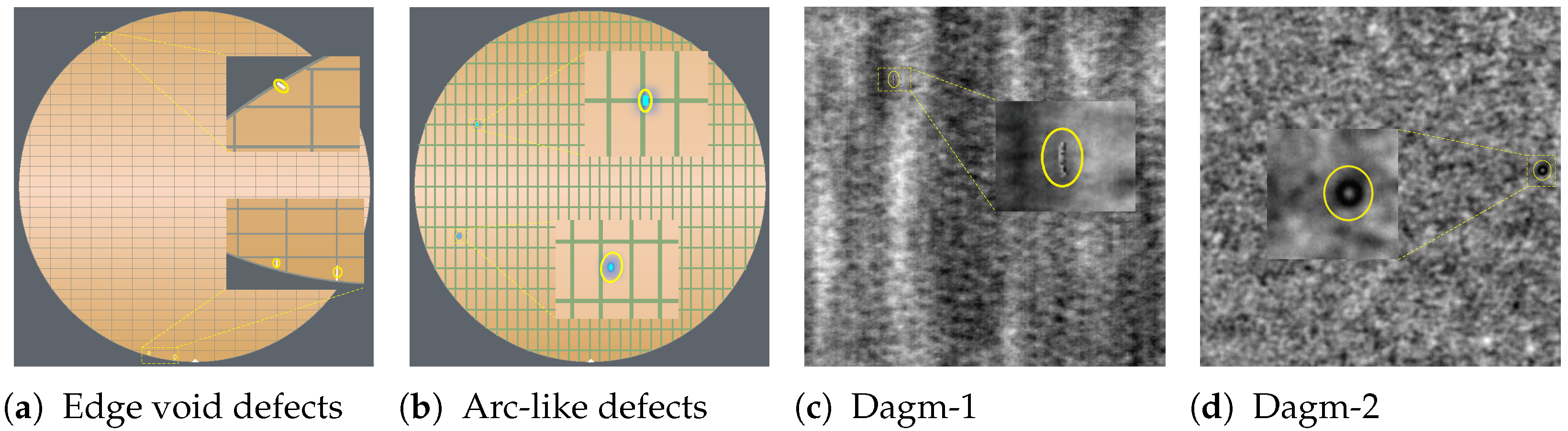
In recent years, numerous deep learning models for object detection have been proposed, such as object detection models [3,4,5,6] and segmentation models [7,8,9] and have demonstrated impressive improvements in detecting objects. However, they suffer from a performance bottleneck on detecting small objects [10,11] due to several factors. First, small objects have a limited number of pixels to represent information. Additionally, small objects are scarce in the training dataset [10,12]. Furthermore, key features that can be used to distinguish small objects from a background or other categories are vulnerable or even lost while going through deep layers of networks, such as convolution or pooling layers [13]. Figure 1 presents examples of small defects we explore in this work, which have these previously mentioned challenges. In these industrial inspection datasets, the sizes of defects range from 3 × 3 to 31 × 31 pixels and smaller than 16 × 16 on average. Moreover, there are usually fewer than four small defects in each image.

Several studies proposed techniques such as multi-scale feature learning [15,16], scale normalization [17,18], or introducing super-resolution networks [19,20] to address the challenges of small object detection. However, these deep learning models require a large number of labeled data for training, while only a limited number of labeled data is available in practical applications. Meanwhile, manual labeling is inherently expensive, time-consuming, and especially challenging and error-prone for small defects. To ease the effort of acquiring a large number of labels, semi-supervised learning (SSL) is a natural fit as SSL offers a promising paradigm that leverages unlabeled data to improve model performance [21]. However, much of recent progress in SSL has focused on image classification tasks, such as [21,22,23,24]. In our case, it is vital to obtain accurate, pixel-level labels to understand the number of dies impacted by the defect. Thus, we formalize the task of detecting small defects as a segmentation problem.

There have been several approaches proposed for semi-supervised semantic segmentation [25,26,27,28]. However, they are mostly consistency-regularization-based methods, which enforce the network output to be invariant to the input perturbations [25,26,27]. Though these methods have reported encouraging results, they become less effective for small defects as the information contained in the few pixels of a small defect can be lost due to perturbations of the input.

Pseudo labeling [29] is another SSL strategy to utilize the limited labeled data to predict labels for unlabeled data, where the model is encouraged to produce high-confidence predictions. While it is a simple heuristic and does not require augmentations, some prior works suggest that pseudo labeling alone is not competitive as other SSL methods [30]. The reason is due to poor network calibration, or threshold setting used in the conventional pseudo labeling methods usually resulting in many incorrect pseudo labels, which in turn leads to a poor generalization of a model [24]. In this work, we use incorrect pseudo labels and noisy pseudo labels or noisy predictions in pseudo labeling interchangeably. Several works propose to combine pseudo labeling with consistency training, such as [28,31]. However, these proposed methods are primarily for medium or large objects and are often unsuitable for small defects. For example, PseudoSeg [28] uses multiple predictions obtained from class activation map (CAM) [32] to calibrate pseudo labels. However, CAM is ineffective in locating the target regions of small defects due to too few pixels contained in small defects. In other words, CAM cannot provide multiple reliable predictions for pseudo labels calibration, thus making PseudoSeg [28] less effective in detecting small defects.

To address these challenges and limitations, we propose a distribution-aware pseudo labeling method (DAP-SDD) to detect small defects precisely while effectively using limited labeled data. To the best of our knowledge, there is no existing method based on distribution-aware pseudo labeling for a semantic segmentation model. Our key contributions are summarized as follows:

• We propose a distribution-aware pseudo labeling method for small defect detection (DAP-SDD) that maximizes the use of the limited number of labels available. Bootstrapping is applied on the limited available labels to obtain an approximate distribution of the complete labels, effectively guiding the pseudo labeling propagation.
• We utilize the approximate distribution in conjunction with t-distribution confidence interval and adaptive training strategies in our proposed threshold setting method, thereby dynamically generating more pseudo labels with high confidence while reducing confirmation bias.
• We conduct extensive experiments on various datasets to validate the proposed method. The evaluation results demonstrate the effectiveness of our proposed approach that outperforms the state-of-the-art techniques.

2. Related Work

Small Object Detection. In recent years, numerous deep learning models such as [3,4,5,6] have been proposed and demonstrated impressive progress on detection performance. However, these models focus on tuning for detecting general objects, mostly of medium or large size, thus suffering from a performance bottleneck for small object detection. There are several approaches proposed to address the challenges of detecting small objects. For example, Kisantal et al. [12] applied data augmentation techniques to increase the number of small objects to improve the detection performance of the model. The authors of [15,16,33] used a multi-scale feature pyramid and deconvolution layers to improve detection performance on small and large objects. SNIP [17] proposed scale normalization and [34] used a dilated convolution network to improve the performance of detecting small objects. These approaches aimed to mitigate the imbalanced distribution of small objects from conventional object sizes. However, they still require a substantial amount of labeled data for training, which is not viable when limited labeled data are available.

Semi-supervised Semantic Segmentation. There are two common strategies used in SSL: consistency regularization and entropy minimization. In consistency regularization-based methods, the prediction is enforced to be consistent when using data augmentation for input images [25], perturbation for embedding features [26], or different networks [35]. While these methods reported impressive detection performance, they become less effective for small defects because of a limited number of pixels in small objects, which could be ignored or even lost when the input or embedding features are perturbed in consistency regularization-based methods. In this way, the model fails to learn key features to distinguish small defects from the background or other categories. On the other hand, entropy minimization encourages a model to predict low-entropy outputs for unlabeled data. Pseudo labeling [29] is one of the implicit entropy minimization methods [36]. Pseudo labeling is usually used with a high confidence threshold setting to reduce the introduction of noisy predictions. With more high confidence information incorporated, the model would learn to minimize output entropy better. However, due to suboptimal threshold setting mechanisms in the conventional pseudo labeling methods [24], some prior works suggest pseudo labeling on its own is not competitive as other SSL methods [30]. Ref. [28] combines consistency regularization with pseudo labeling to improve model performance. However, it still requires consistency regularization, which is ineffectual for small defects. Our design of pseudo labels is inspired by recent SSL-based image classification works [21,22,23], which incorporated distribution alignment to generate high confidence pseudo labels for unlabeled data. While these approaches require data augmentation to generate multiple class distributions for distribution alignment or comparison, our method does not require data augmentation during pseudo labeling. In addition to these two main categories of SSL methods, several GAN-based models are proposed. For example, Souly et al. [37] generates additional training data via GAN to alleviate the lack of labeled data. Hung et al. [38], on the other hand, uses an adversarial network to learn a discriminator between the ground truth and the prediction to generate a confidence map. Unlike GAN-based models, which require adversarial networks to generate additional data, our method directly generates labels via proper threshold setting without introducing extra data.

3. Methodology

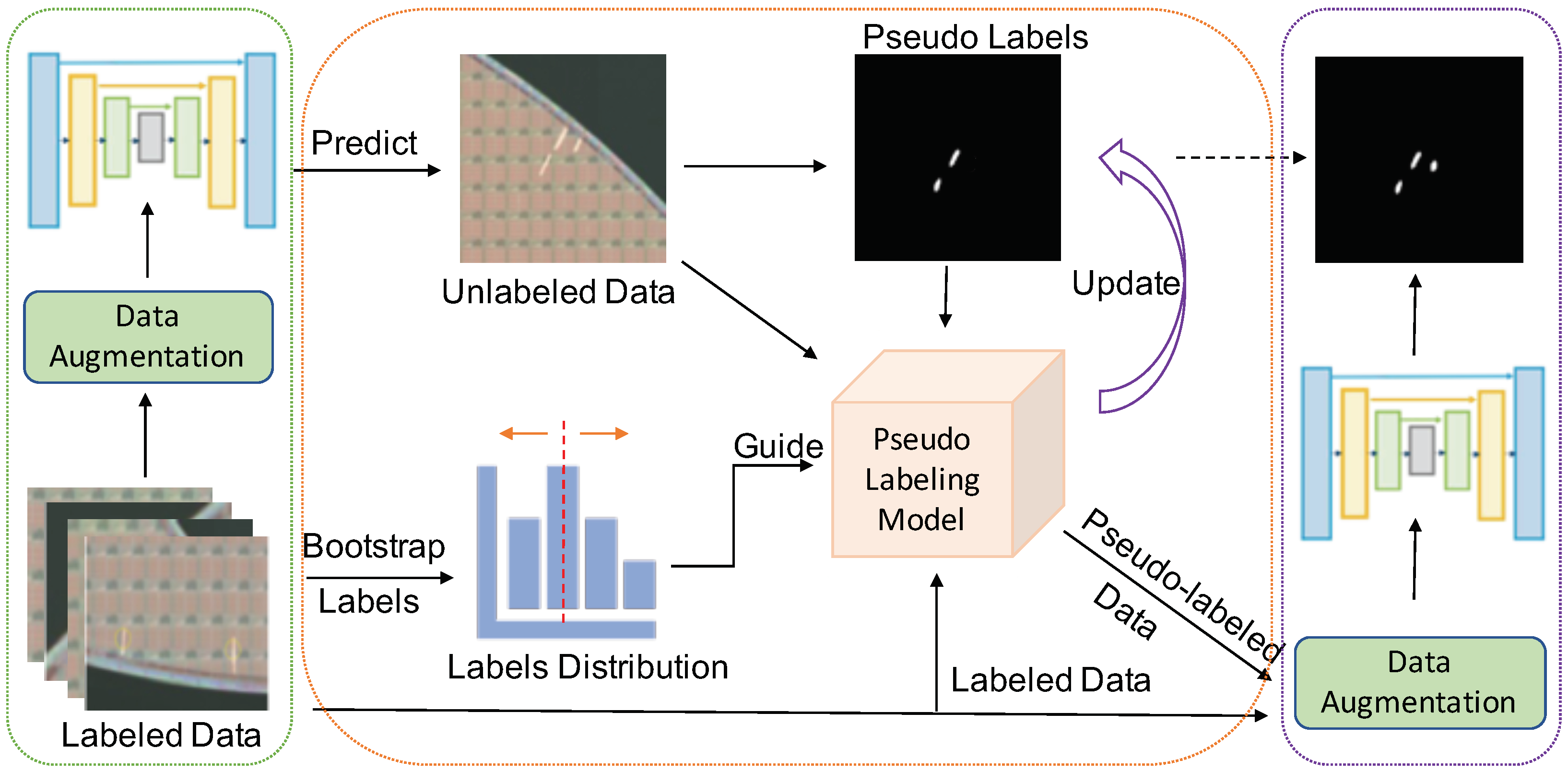
Figure 2 depicts an overview of our proposed method: distribution-aware pseudo labeling for small defect detection (DAP-SDD).

3.1. Leverage Labeled Data

Data augmentation can usually help improve detection performance, and there are several commonly used augmentation techniques we could employ, such as random crop, rotation, horizontal flip, color jittering, mixup, etc. [28,40]. However, these commonly-used techniques become incompetent in improving model performance when limited labels are available, e.g., less than 5% of the fully-labeled dataset. Inspired by augmentation techniques proposed in [12,41], we rotate images by 0, 90, 180, 270 degrees to quadruple labeled data. Unlike augmenting images by directly copy-pasting multiple times as in [12], our variants of original data not only enrich the labeled data but also can help prevent the model from becoming biased when the amount of pseudo labeled data increases during pseudo label propagation.

3.2. Distribution-Aware Pseudo Labeling

In pseudo labeling methods, one common way is to convert model predictions to hard pseudo labels directly. To illustrate this, let $D_l=\{x_l^{\left(i\right)},y_l^{\left(i\right)}\}$ be a labeled dataset and $D_u=\left\{x_u^{\left(i\right)}\right\}$ be a unlabeled dataset. We first train a model $f_{\theta }$ on $D_l$ and use the trained model to infer on $D_u$. Let us further denote $p\left(x_u^{\left(i\right)}\right)$ as the prediction of unlabeled sample $x_u^{\left(i\right)}$, then the pseudo label for $x_u^{\left(i\right)}$ can be denoted as:

$${\tilde{y}}_u^{\left(i\right)}=\mathfrak{1}[p\left(x_u^{\left(i\right)}\right)>\gamma ],$$

(1)

where $\gamma \in (0,1)$ is a threshold to generate pseudo labels. Note that, for a semantic segmentation model such as ours, $p\left(x_u^{\left(i\right)}\right)$ is a probability map and ${\tilde{y}}_u^{\left(i\right)}$ is a binary mask with pseudo labels. As Equation (1) shows, threshold setting is critical to generate reliable pseudo labels. However, determining an optimal threshold is difficult, and a sub-optimal threshold value can introduce many incorrect pseudo labels, which degrades model performance. Therefore, we propose a novel threshold setting method, which can generate more pseudo labels with high confidence without bringing many noisy predictions.

3.2.1. Bootstrap Labels

Assuming the distribution of limited labeled data approximates that of fully labeled data, we first apply bootstrapping, a resampling technique that estimates summary statistics (e.g., mean and standard deviation) on a population by randomly sampling a dataset with replacement. The metric we employed in bootstrapping is $label\_pixel\_ratio$, which is denoted as:

$$label\_pixel\_ratio=\frac{label\_pixels}{image\_pixels},$$

(2)

where $label\_pixels$ is the number of pixels of one label, and the $image\_pixels$ is the number of pixels of the image in which the label locates. For example, if the number of pixels of one label is 256, and the image size is $2048\times 2048$, then the $label\_pixel\_ratio$ for this label is $256/(2048\times 2048)=0.00006104$.

3.2.2. Distribution-Aware Pseudo Label Threshold Setting

Once we obtain the mean of $label\_pixel\_ratio$ ($\mu$) in the previous step, we calculate the number (k) of pixels of predictions on $D_l$ ($p\left(D_l\right)$), and the top k of sorted $p\left(D_l\right)$ are pixels for labels. In other words, the threshold for $D_l$ is the k-th value in $p\left(D_l\right)$, which we use to set the threshold for unlabeled data $D_u$ as well. This mechanism works as both labeled and unlabeled data are supposed to be sampled from the same distribution of fully labeled data and share the same mean of label distribution. We also use the same trained model to infer on them. The k at a specific iteration n with the predictions of $p_n\left(D_l\right)$ is given by:

$$k_{n,base}=\lfloor \mathcal{N}\left(p_n\left(D_l\right)\right)*\mu \rceil ,$$

(3)

where $\mathcal{N}\left(p_n\left(D_l\right)\right)$ is used to obtain the total number of pixels in $p_n\left(D_l\right)$. The raw outcome from this equation is a real number, so we round it to the nearest integer to obtain $k_{n,base}$. Then, the corresponding $k_{n,base}$-th value in $p_n\left(D_l\right)$ can be used for threshold setting.

Using Equation (3), we can set a quite reasonable initial threshold as the calculation utilizes the mean of estimated label distribution. However, as the pseudo labeling model is encouraged to produce more high-confidence (i.e., low-entropy) predictions as training continues, this method alone may suffer from an insufficient number of proposed pseudo labels. To incorporate more pseudo labels with high-confidence predictions while reducing the possibility of introducing noisy predictions, we use a confidence interval and gradually increase it. An increasing confidence interval allows incorporating a higher number of confident predictions as high-confidence pseudo labels. Specifically, we use the t-distribution to find a given $100(1-\alpha )\%$ confidence interval ($CI$), which can be obtained via:

$$CI=\mu \pm t_{\alpha /2,m-1}\frac{s}{\sqrt{m}},$$

(4)

where $\mu$ and s are the estimated mean and sample standard deviation of $label\_pixel\_ratio$, respectively. m represents the number of labels and t is a critical value in t-distribution table to obtain $P(T\le t)=1-\alpha /2$ at the degrees freedom of $m-1$. The lower bound of the confidence interval ($C{I}_{lower}$) is $\mu -t_{\alpha /2,m-1}\frac{s}{\sqrt{m}}$, whereas the upper bound ($C{I}_{upper}$) is $\mu +t_{\alpha /2,m-1}\frac{s}{\sqrt{m}}$. We use the t-distribution in our proposed method because of the lack of labeled samples available. In such a case, the estimated standard deviation tends to be farther from the real standard deviation, and t-distribution fits better than the normal distribution. We also present the comparison results of them in the later section of ablation studies. Once we obtain the confidence interval, we can map them to find the lower and upper bound of k via Equation (3) by replacing the $\mu$ with $C{I}_{lower}$ or $C{I}_{upper}$. Then, we can use the $k_{n,ci}$-th value of $p_n\left(D_l\right)$, with a given $100(1-{\alpha }_n)\%$ confidence level to obtain the threshold ${\gamma }_n$ at a specific iteration n:

$${\gamma }_n=\mathcal{K}(p_n\left(D_l\right),\lfloor \mathcal{N}\left(p_n\left(D_l\right)\right)*t_{{\alpha }_n/2,m-1}\frac{2s}{\sqrt{m}}*{\nu }_n\rceil ),$$

(5)

where $\mathcal{K}(p_n,k)$ is a function to find k-th value in $p_n$ and ${\nu }_n$ is an adjustment factor used to slow down or speed up propagation during training.

In addition to using the t-distribution to calculate the confidence interval for setting thresholds, we also employ another intuitive method for selecting high confidence pseudo labels. Specifically, we find the threshold that produces the best performance on labeled data. We then use that threshold to generate initial pseudo labels for unlabeled data. To illustrate this, let $P_{l,0}$ denote the precision obtained from the labeled data, which can be considered as a confidence level for pseudo labels since the precision indicates how many predictions out of all predictions are true small defects. We can increase the confidence level with a moving step $\tau$ as the training goes on. Along with the $k_{n,base}$ via Equation (3), we can obtain the threshold ${\gamma }_n$ at a specific iteration n by using:

$${\gamma }_n=\mathcal{K}(p_n\left(D_l\right),\lfloor \mathcal{N}\left(p_n\left(D_l\right)\right)*\mu *(P_{l,0}+{\nu }_n*\tau )\rceil ).$$

(6)

Overall, the method utilizing t-distribution confidence interval Equation (5) performs better than the intuitive method Equation (6), and their comparison results are presented in the later section of ablation studies.

3.2.3. Training Strategies

During training, we adjust the moving step of pseudo labeling propagation to set threshold adaptively. To accomplish this, we keep monitoring training and use the model evaluation results (e.g., Precision, Recall, F1 score) on labeled data. For example, if the monitored results show a decrease in both F1 score and recall but an increase in precision (close to 1.0), it indicates the threshold is set too high to incorporate more confident pseudo labels. In other words, the model can speed up the propagation and set the adjustment factor $\nu$ to a bigger value so that the threshold will be set to a lower value, thereby incorporating more high-confidence pseudo labels and vice versa. Another strategy we adopt during training is a weighted moving average of thresholds. Due to the random combination of training data batch, a model may temporarily suffer a significant performance decrease in a certain iteration. A weighted moving average of thresholds can prevent such an outlier threshold from resetting the threshold value that the model has learned to ensure more stable pseudo labeling propagation.

Algorithm 1 presents the training procedure of our proposed distribution-aware pseudo labeling. First, we use the labeled data to train a model $f_{\theta ,0}$, and then use the trained model to generate initial pseudo labels and obtain the initial precision $P_{l,0}$. During the iterative pseudo labeling with the maximum number of iterations N, we calculate thresholds ${\gamma }_n$ for each iteration via Equations (5) or (6). Then, we evaluate the obtained thresholds ${\gamma }_n$ and the moving average threshold ${\gamma }_{n-1,ma}$ on labeled data. The threshold that yields better evaluation results (i.e., F1 Score) is selected. Meanwhile, by comparing the evaluation results (Precision, Recall, F1 Score denoted as $P_n,R_n,F{1}_n$, respectively) of the current iteration with that of the previous iteration, we can obtain the adjustment factor ${\nu }_n$ to speed up or slow down pseudo label propagation. Moreover, we update the moving average threshold for the next iteration. Next, we use the selected threshold ${\gamma }_n$ to generate pseudo labels for unlabeled data $D_u$. We then combine the pseudo labeled data $D_p$ with labeled data $D_l$ to retrain the model. We repeat these steps to update pseudo labels iteratively to achieve better detection performance of the model. Once the detection performance from the model reaches a certain threshold (e.g., F1 ≥ 0.85) but remains or decreases beyond that, the warm restart and mixup augmentation will be applied on both labeled data and pseudo labeled data to improve detection performance further.

Algorithm 1 Distribution-Aware Pseudo Labeling.

1: Train a model $f_{\theta ,0}$ using labeled data $D_l$.

2: for $n=1,2,\dots ,N$ do

3:     Obtain threshold ${\gamma }_n$

4:     $P_n,R_n,F{1}_n,{\nu }_n,{\gamma }_n\leftarrow E(D_l,{\gamma }_n,{\gamma }_{n-1,ma})$

5:     ${\gamma }_{n,ma}\leftarrow M({\gamma }_n,{\gamma }_{n-1},{\gamma }_{n-2},\alpha ,\beta )$

6:     $D_{p,n}\leftarrow$ Pseudo label $D_u$ using ${\gamma }_n$

7:     $\tilde{D}\leftarrow D_l\cup D_{p,n}$

8:     Train $f_{\theta ,n}$ using $\tilde{D}$.

9:     $f_{\theta },D_p\leftarrow f_{\theta ,n},D_{p,n}$

10: end for

11: return $f_{\theta },D_p$

3.2.4. Loss Function

During pseudo labeling propagation, the loss function ${\mathcal{L}}_p$ incorporates labeled and pseudo labeled data, which can be denoted as:

$${\mathcal{L}}_p=-\left(\sum _{D_l}\mathcal{L}(y_l,{\widehat{y}}_l)+\eta \sum _{D_u}\mathcal{L}(y_p,{\widehat{y}}_p)\right),$$

(7)

where $y_l$ is the ground truth labels, and $y_p$ represents pseudo labels. ${\widehat{y}}_l$ and ${\widehat{y}}_p$ denote the predictions of labeled data and unlabeled data, respectively. $\mathcal{L}$ represents the cross-entropy loss function. As the pseudo labeling progresses, the amount of pseudo labeled data will increase accordingly. To avoid the model increasingly favoring pseudo labeled data over the original labeled data, we add a weight $\eta \in (0,1)$ to adjust the impact from pseudo labels. In practice, we can achieve this by repeatedly sampling or using the similar augmentation techniques described in Section 3.1.

During the training process using mixup augmentation, we define a mixup loss function ${\mathcal{L}}_m$, which is given by:

$${\mathcal{L}}_m=-\sum _{i=1}^N\left(\lambda \mathcal{L}(y_a^{\left(i\right)},{\widehat{y}}_a^{\left(i\right)})+(1-\lambda )\mathcal{L}(y_b^{\left(i\right)},{\widehat{y}}_b^{\left(i\right)})\right),$$

(8)

$y_a$ and $y_b$ are the original labels of the input images, and ${\widehat{y}}_a$ and ${\widehat{y}}_b$ are corresponding predictions. N is the number of samples used for training. In the first step of leveraging labeled data, N only includes the number of labeled data, while in the last step, both the labeled and pseudo labeled data will be included. $\lambda \in [0,1]$ is used in mixup augmentation for constructing virtual inputs and outputs [40]. Specifically, the mixup uses the following rules to create virtual training examples:

$$\tilde{x}=\lambda \times x_a+(1-\lambda )\times x_b$$

$$\tilde{y}=\lambda \times y_a+(1-\lambda )\times y_b,$$

where $(x_a,y_a)$ and $(x_b,y_b)$ are two original inputs drawn at random from training batch, $\lambda \in [0,1]$ and the $\tilde{x}$ and $\tilde{y}$ are constructed input and corresponding output.

4. Results and Discussion

4.1. Datasets

We use an in-house dataset from the wafer inspection system (WIS) in our evaluation. This dataset contains two types of small defects on wafer images: edge void and arc-like defects. Each of them has 213 images: 173 for training and 40 for test. There are 618 labels for edge void and 406 labels for arc-like, weak labels from the current system tool and verified predictions from a trained model. The image size is 2048 × 2048, and we crop it into 512 × 512 patches to fit into GPU memory.

We also evaluate our method on two public datasets: industrial optical inspection dataset of DAGM 2007 [14] and tiny defect detection dataset for PCB [42]. We use Class 8 and Class 9 of DAGM as they fit into a small defect category (denoted as Dagm-1 and Dagm-2). We split each class into two sets of 150 defective images in gray-scale for training and testing. The image size is 512 × 512 in DAGM. The defects are labeled as ellipses, and each image has one labeled defect.

On the other hand, the PCB dataset includes six types of tiny defects (missing hole, mouse bite, open circuit, short, spur, and spurious copper), and each image may have multiple defects. PCB contains 693 images with defects: 522 and 101 images for training and test, respectively. The total number of defects is 2953. There are different sizes of PCB images, and the average pixel size of an image is 2777 × 2138. We also crop it into 512 × 512 patches for training.

4.2. Evaluation Metrics

Intersection over Prediction (IoP). In this work, instead of using IoU (intersection over union), we adopt IoP (intersection over prediction) [43] to overcome the issue shown in Figure 1, where one weak label may contain multiple small defects or cover more area than the true defect area. IoP is defined as the intersection area between ground truth and prediction divided by the area of prediction. If the IoP of a prediction for a small defect is greater than a given threshold (0.5 in this work), we count it as a true positive; otherwise, we count it as a false positive. If one weak label contains multiple true positive predictions, we only count it as one true positive.

Average Precision (AP), F1 Score. We use AP (average precision) and F1 Score to evaluate the performance of small defect detection.

4.3. Experimental Settings and Parameters

In this work, we adopt a commonly-used segmentation model U-Net [8] in our proposed method, which has been proven to be effective in medical image segmentation tasks, such as detecting microcalcifications in mammograms [43,44]. Moreover, U-Net has a relatively small size of model parameters, which is favorable in practical use. U-Net consists of three downsampling blocks and three upsampling blocks with skip connections. Each block has two convolution layers, and each of them is followed by batch normalization and ReLU. As our proposed pseudo labeling strategy is not confined to a specific deep learning model, it can be easily implemented in other deep neural networks. We will extend our proposed techniques to other segmentation models in future work.

We use the Adam optimizer in the model training. The initial learning rate is set to 1 × 10${}^{-3}$ and gradually decreases during training. The adjustment factor ${\nu }_n$ is set to 1.1 to speed up pseudo label propagation or set to 0.9 to slow down the propagation. The moving average weights $[\alpha ,\beta ,(1-\alpha -\beta \left)\right]$ are set to $[0.5,0.3,0.2]$ for the current iteration threshold ${\gamma }_n$ and thresholds of previous two iterations ${\gamma }_{n-1},{\gamma }_{n-2}$, respectively. The t-distribution confidence interval ranges from 0.5 to 0.995 with a moving step of 0.005.

4.4. Experiment Results

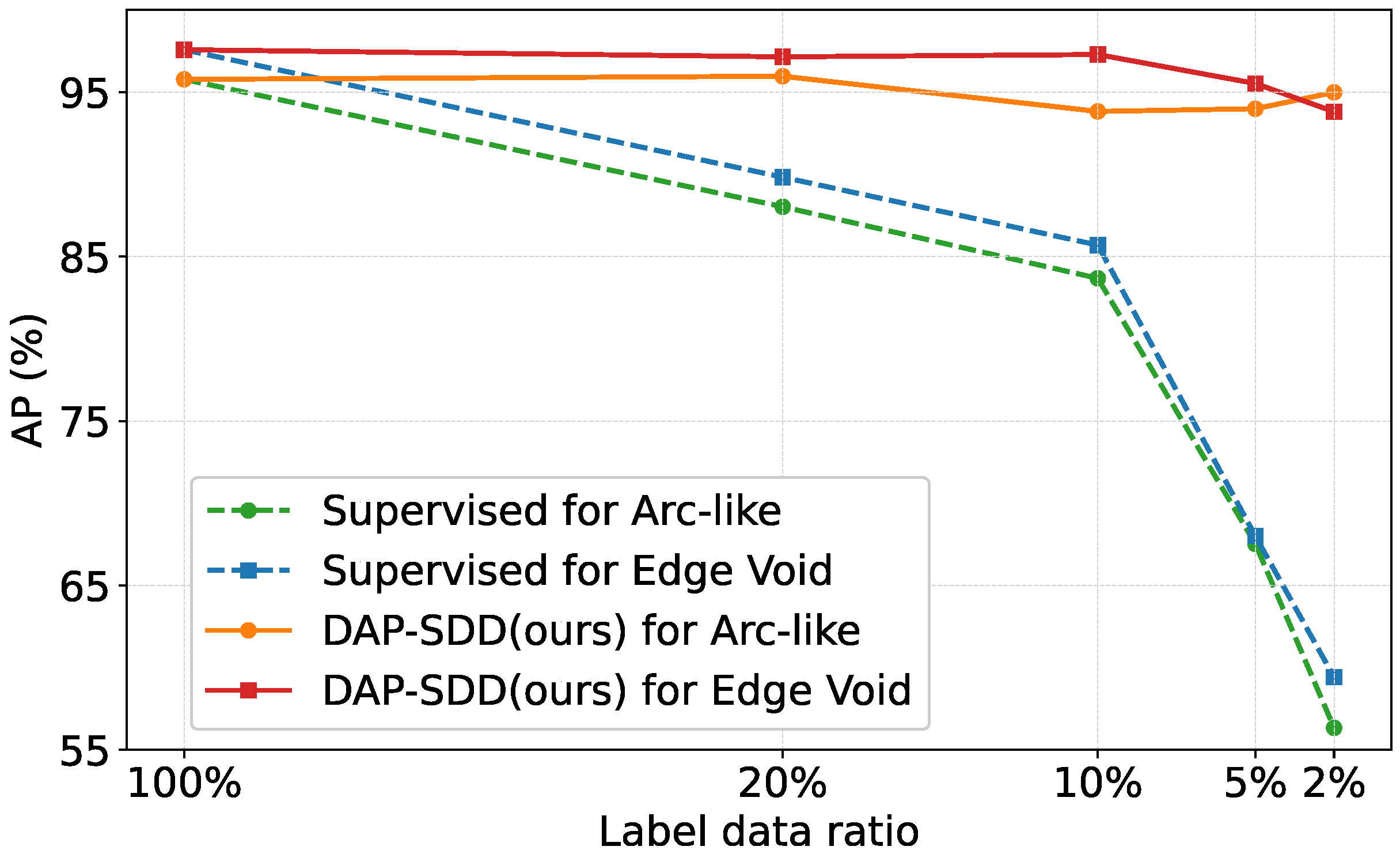
We first evaluate our proposed method on two different types of small defects on wafer images (the WIS dataset). Figure 3 demonstrates the improvements brought by our method over the supervised baseline. Overall, our proposed method can achieve above 0.93 of AP for a different amount of labeled data available and obtain comparable results as a fully-labeled (100%) dataset even when the labeled data ratio is 2% (four labeled images). However, the detection performance of the supervised method decreases dramatically when the labeled data size is limited. For instance, the AP reduces to below 0.6 when 2% of labeled data is available.

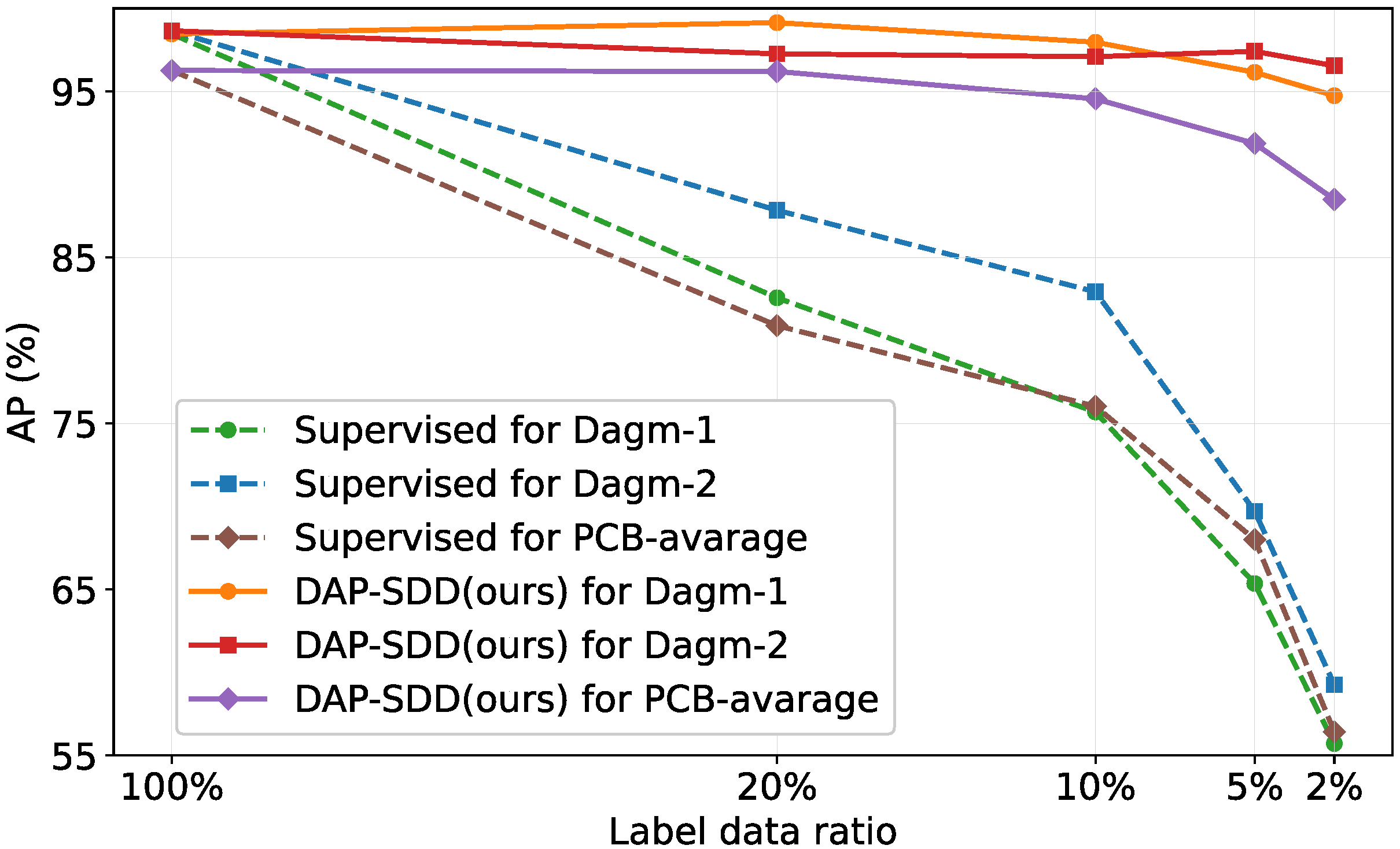
Figure 4 demonstrates the improvements by our method (solid lines) over the supervised baseline (dash lines) on the DAGM and PCB datasets. Similar to the results of the WIS dataset, our proposed method can achieve comparative results of fully-labeled (100%) when the labeled data ratio is 10% on different small defects in DAGM and PCB datasets. The average precision (AP) by our method remains above 0.9 when only 5% of labeled data are available while the AP by the supervised model degrades dramatically. Note that in Figure 4, the values of PCB-average represent the average AP of six different types of defects in the PCB datasets.

We then compare our method with state-of-the-art semi-supervised semantic segmentation methods.

Table 1. Comparison with state-of-the-art methods on the WIS dataset with 10% of labeled data.

Method	Edge Void		Arc-Like
	AP (%)	F1 (%)	AP (%)	F1 (%)
CCT (Ouali et al.)	-	-	-	-
CCT+Pseudo (Ouali et al.)	70.75	69.80	71.09	72.13
AdvSemSeg (Hung et al.)	76.61	76.42	76.98	79.51
Self-training (Zoph et al.)	89.29	88.14	85.34	86.89
DAP-SDD (Ours)	97.29	96.64	94.99	91.38

shows the comparison results on the Edge Void defect dataset with 10% of labeled data. CCT [26] is a consistency regularization-based method. As shown in Table 1, the CCT alone fails to recognize and locate small defects. CCT also provides a way of training with offline pseudo labels. So, we use the pseudo labels generated from the first step of our method. As we can see, CCT+Pseudo improves the detection performance as more pseudo labeled data are incorporated. However, the initial pseudo labels might contain incorrect labels, which are not updated iteratively in CCT. Therefore, CCT+Pseudo still presents relatively low detection performance. AdvSemSeg [38], however, uses an adversarial network for semi-supervised semantic segmentation. The experiment results show that AdvSemSeg performs better than CCT, which indicates adversarial network can be a potential direction for improving small defect detection. However, due to limited ground truth labels, AdvSemSeg does not perform well as reported in [38]. In self-training, we exclude the labeled data and only use the initial pseudo labels as the supervisory signals for unlabeled data. During self-training, instead of setting pseudo labels based on pixel confidence score higher than 0.5 as in [45], we adopt the same threshold setting strategies as our method to generate pseudo labels for self-taught training effectively. As shown in Table 1, self-training shows significantly better AP and F1 scores than CCT and AdvSegSeg. Overall, DAP-SDD achieves the highest AP and F1 scores. We attribute this to the fact that ours also incorporates labeled data that contain useful prior knowledge.

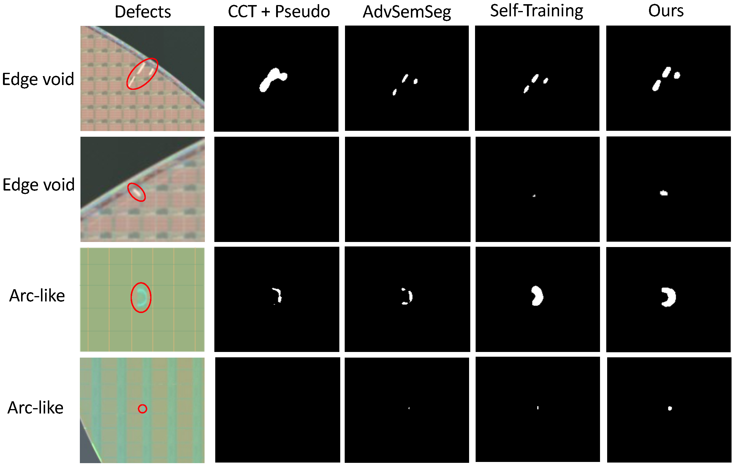
In Figure 5, we present examples of predicted labels for small defects generated by different methods. We can observe that all the evaluated models can generate labels for relatively large defects, as shown in the first row of edge void defects and the third row of arc-like defects. Compared to CCT+Pseudo or AdvSemSeg, which generate incomplete labels or overfull labels, self-training and our proposed method obtain more accurate labels. However, for the significantly tiny or dim defects, such as ones shown in the second row and fourth row, most of these models suffer from missing detection while our method can still detect them. Overall, our proposed method performs best regardless of the different sizes of small defects.

The prediction results and comparison results with state-of-the-art methods on the DAGM and PCB datasets are shown in

Table 2. Evaluation results (AP, %) on public datasets (DAGM, PCB) when different amounts of labeled data are available. Total data amount (100%): DAGM (552), DAGM (150).

Data Amount	DAGM		PCB
	Dagm-1	Dagm-2	Missing Hole	Mouse Bite	Open Circuit	Short	Spur	Spurious Copper	Average
100%	98.46	98.65	98.75	96.03	95.34	98.57	96.38	92.46	96.26
20%	99.14	97.26	98.54	94.71	96.45	94.03	97.19	96.27	96.20
10%	97.96	97.09	97.35	93.98	91.75	92.77	95.28	96.19	94.55
5%	96.15	97.41	97.13	89.10	86.07	89.92	91.95	96.98	91.86
2%	94.74	96.54	95.67	87.71	83.07	85.79	88.32	90.38	88.49

and

Table 3. Comparison with state-of-the-art methods on public datasets (DAGM, PCB), evaluation metric: AP (%).

Data Amount	DAGM		PCB
	Dagm-1	Dagm-2	Missing Hole	Mouse Bite	Open Circuit	Short	Spur	Spurious Copper	Average
CCT [26]	69.55	66.07	63.81	57.84	55.72	56.39	63.61	63.67	62.08
CCT+Pseudo [26]	83.15	82.79	79.37	73.32	70.18	72.46	79.40	76.99	75.29
AdvSemSeg [38]	84.62	85.68	84.28	80.71	80.44	82.10	83.45	83.75	82.46
Self-training [45]	92.59	91.18	88.15	85.84	86.83	85.67	87.92	87.41	86.97
DAP-SDD (Ours)	97.96	97.09	97.35	93.98	91.75	92.77	95.28	96.19	94.55

.

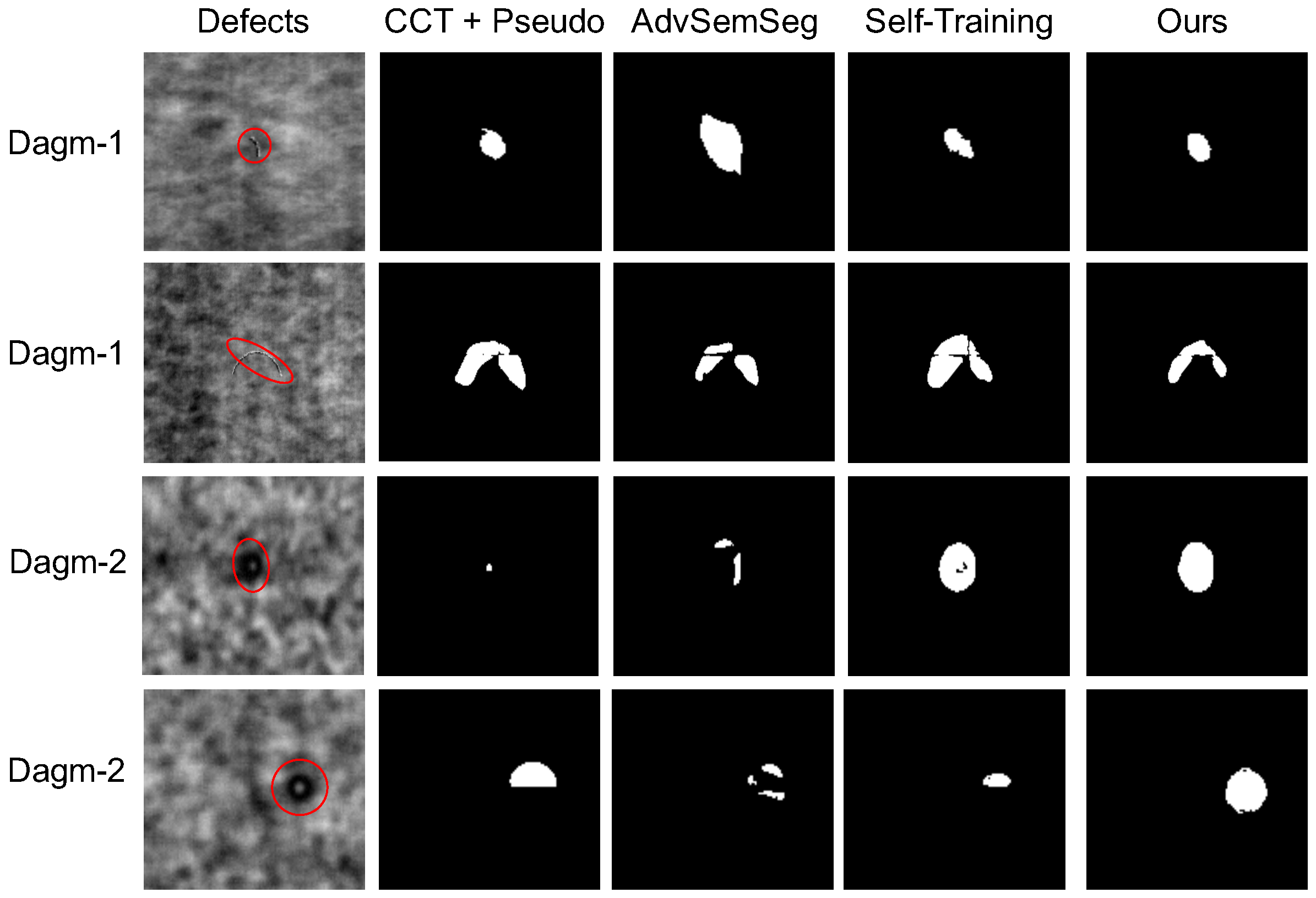
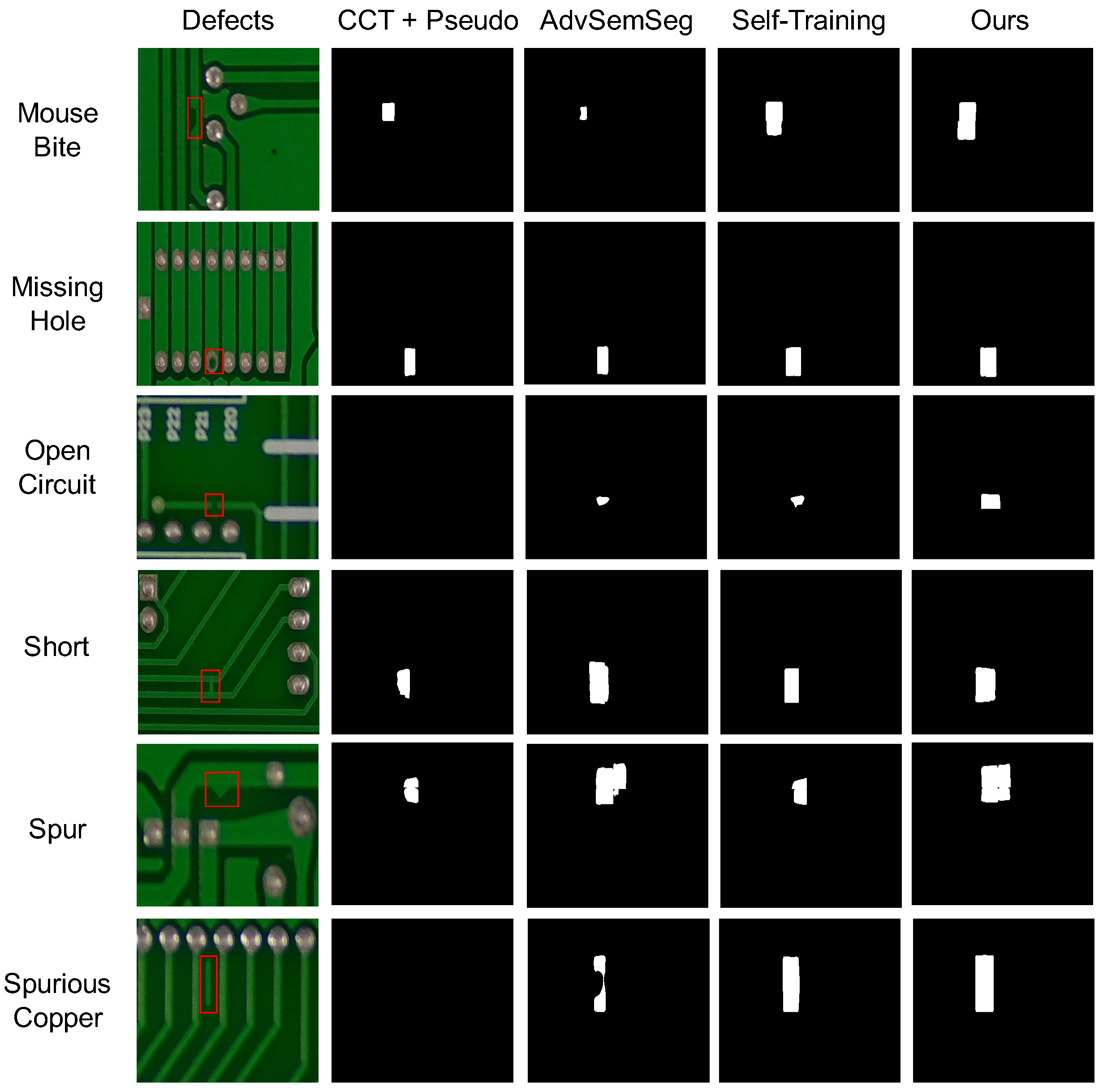
Moreover, we present examples of predicted labels for small defects in the DAGM (Figure 6) and PCB datasets (Figure 7) generated by different methods. As the results have shown, our proposed method consistently outperforms the state-of-the-art semi-supervised segmentation models on various datasets with various types of defects.

4.5. Ablation Studies

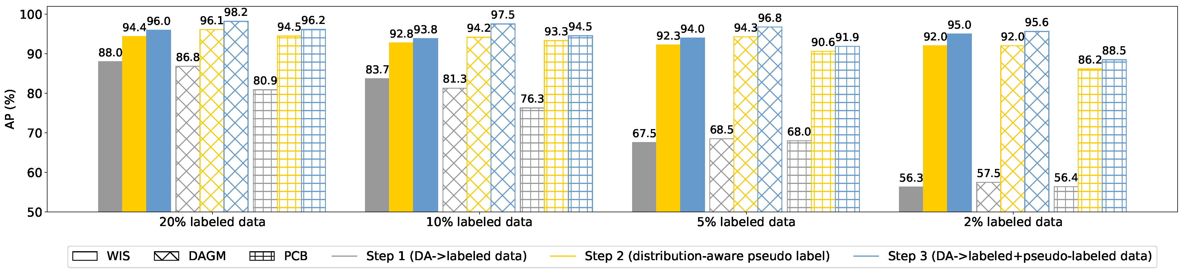
Contribution of components for performance improvement.Figure 8 demonstrates how different components in our proposed method contribute to detection performance on both in-house and public datasets. For a fair comparison, we use the same data augmentations in the supervised baseline and ours. Therefore, the results of the first step using only labeled data are also supervised baseline. As shown in Figure 8, for the WIS dataset (solid bars), the model using 20% of labeled data can achieve around 88% of AP, which is still lower than our target (our real-world applications typically require AP of 90% or higher). When we have 2% of labeled data available, the AP value decreases to 56%. In Step 2, utilizing the proposed distribution-aware pseudo labeling method significantly improved the detection performance for all cases, and cases with fewer labeled data benefit more. For example, AP is improved from 56% to 92% when using 2% of labeled data. The results demonstrate that our proposed method can effectively leverage the information from massive unlabeled data to improve detection performance. In the final step, warm restart and mixup are employed to improve performance further. We obtain similar results on public datasets shown in Figure 8 (bars with patterns). Overall, the proposed distribution-aware pseudo labeling contributes most significantly to the detection performance and the data augmentations we adopted in DAP-SDD are effective in enhancing the model’s performance and robustness.

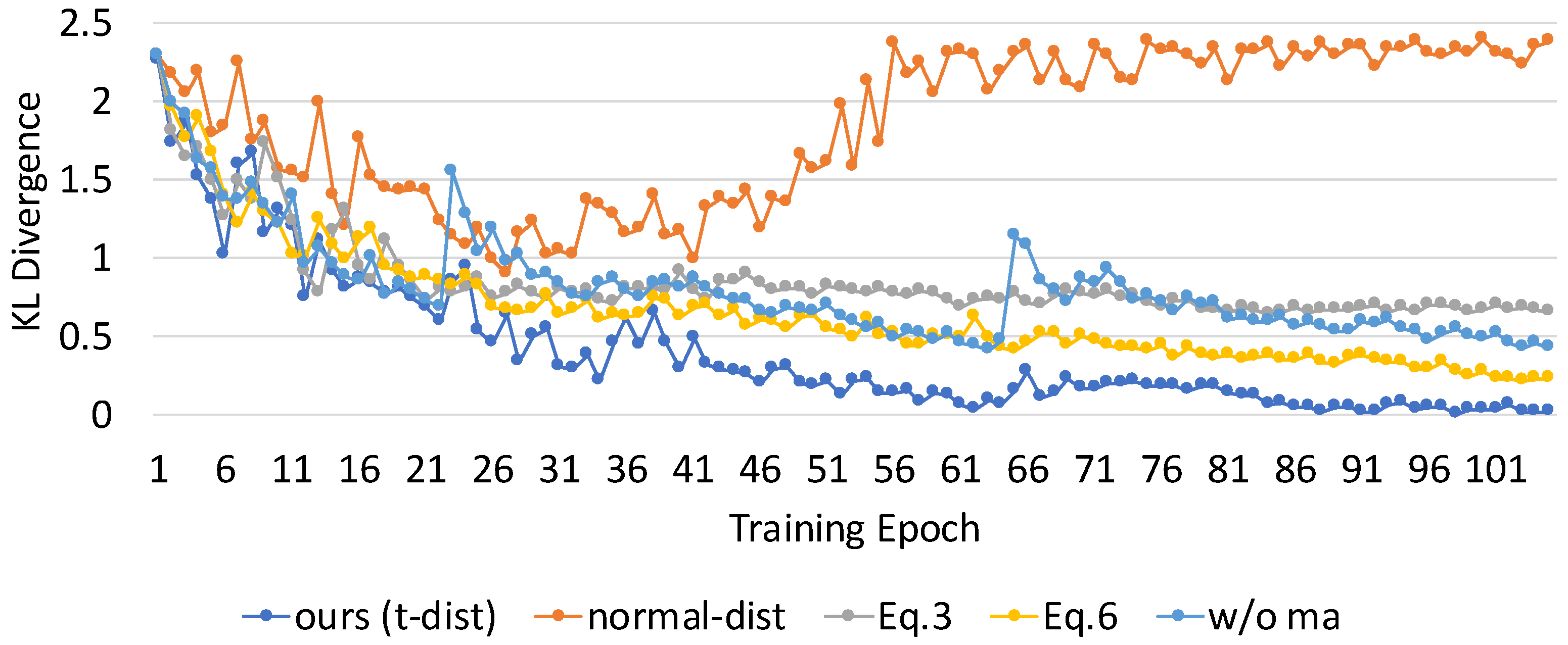
Compare with more baselines. In our proposed DAP-SDD, we assume the distribution of proposed labels approximates the distribution of ground truth labels as training proceeds. We use the Kullback–Leibler (KL) divergence to evaluate the differences in the distribution of proposed labels compared with ground truth labels during training, which is shown in Figure 9. The KL divergence is a commonly-used measurement for evaluating how one probability distribution differs from the other reference distribution. We can observe that: (a) t-dist vs. normal-dist: t-distribution (t-dist) performs better than a normal distribution (normal-dist) because t-dist has heavier tails. Thus it is more suitable for estimating the confidence interval (CI) when the sample size is limited as in our cases. For a given CI range, normal-dist tends to incorporate more predictions than t-dist, which in turn brings ‘too many’ noisy predictions for pseudo labels. As a result, the accumulated noisy impact overwhelms that of original limited labels as training proceeds. (b) Adaptive vs. fixed threshold: adaptive thresholding that combines Equation (3) and Equation (5) can keep the model learning more useful information during training and outperforms the fixed threshold obtained via Equation (3). (c) Equation (5) vs. Equation (6): Equation (6) is more conservative in incorporating confident predictions than Equation (5) when using the same moving step (0.005), and it requires more training epochs to reach the equivalent results as Equation (5). (d) with vs. without ma: compared with the baseline without moving average (ma) threshold, our method incorporates ma, which helps prevent outlier thresholds (e.g., epochs 23 and 65) from resetting what the model has learned. In addition, the corresponding detection performance and KL divergence at the same training epoch (100th) of these baselines are shown in

Table 4. Comparison of detection performance (AP, %) and KL divergence (same training epochs 100) on various baselines.

Baseline Method	AP (%)	KL Divergence
Normal distribution	66.52	2.3772
Fixed threshold Equation (3)	81.63	0.6528
DAP-SDD via Equation (6)	94.34	0.2288
DAP-SDD w/o ma	86.98	0.4181
DAP-SDD (t-dist, Equation (5), ma)	97.29	0.0127

. As we can observe, DAP-SDD using the t-distribution confidence interval and with moving average achieves the best detection performance while having the smallest KL divergence.

5. Conclusions

In this work, we propose a distribution-aware pseudo labeling for small defect detection (DAP-SDD) when limited labeled data are available. We first applied bootstrapping for the available labeled data to approximate the distribution of the whole labeled dataset. Then, we used it to guide pseudo label propagation. Our proposed method incorporates t-distribution confidence interval and adaptive training strategies, and thus can effectively generate more pseudo labels with high confidence while reducing confirmation bias. The extensive experimental evaluation on various datasets with various types of defects has demonstrated that our proposed DAP-SDD consistently outperforms the state-of-the-art techniques with above 0.9 of average precision and up to 0.99. Our in-depth analysis of the ablation studies clearly shows how each component employed in our approach effectively utilizes the limited labeled data.

References

- Shankar, N.; Zhong, Z. Defect detection on semiconductor wafer surfaces. Microelectron. Eng. 2005, 77, 337–346. [Google Scholar] [CrossRef]
- Huang, S.H.; Pan, Y.C. Automated visual inspection in the semiconductor industry: A survey. Comput. Ind. 2015, 66, 1–10. [Google Scholar] [CrossRef]
- Ren, S.; He, K.; Girshick, R.; Sun, J. Faster R-CNN: Towards Real-Time Object Detection with Region Proposal Networks. Adv. Neural Inf. Process. Syst. 2015, 28, 91–99. [Google Scholar] [CrossRef] [PubMed] [Green Version]
- Redmon, J.; Farhadi, A. YOLOv3: An Incremental Improvement. arXiv 2018, arXiv:1804.02767. [Google Scholar]
- He, K.; Gkioxari, G.; Dollár, P.; Girshick, R. Mask R-CNN. In Proceedings of the 2017 IEEE International Conference on Computer Vision (ICCV), Venice, Italy, 22–29 October 2017; pp. 2980–2988. [Google Scholar] [CrossRef]
- Lin, T.; Goyal, P.; Girshick, R.; He, K.; Dollár, P. Focal Loss for Dense Object Detection. In Proceedings of the 2017 IEEE International Conference on Computer Vision (ICCV), Venice, Italy, 22–29 October 2017; pp. 2999–3007. [Google Scholar] [CrossRef] [Green Version]
- Long, J.; Shelhamer, E.; Darrell, T. Fully convolutional networks for semantic segmentation. In Proceedings of the 2015 IEEE Conference on Computer Vision and Pattern Recognition (CVPR), Boston, MA, USA, 7–12 June 2015; pp. 3431–3440. [Google Scholar] [CrossRef] [Green Version]
- Ronneberger, O.; Fischer, P.; Brox, T. U-Net: Convolutional Networks for Biomedical Image Segmentation. In International Conference on Medical Image Computing and Computer-Assisted Intervention; Springer: Cham, Switzerland, 2015. [Google Scholar]
- Chen, L.C.; Zhu, Y.; Papandreou, G.; Schroff, F.; Adam, H. Encoder-Decoder with Atrous Separable Convolution for Semantic Image Segmentation. In Proceedings of the European Conference on Computer Vision (ECCV), Munich, Germany, 8–14 September 2018. [Google Scholar]
- Tong, K.; Wu, Y.; Zhou, F. Recent advances in small object detection based on deep learning: A review. Image Vis. Comput. 2020, 97, 103910. [Google Scholar] [CrossRef]
- Fu, K.; Li, J.; Ma, L.; Mu, K.; Tian, Y. Intrinsic Relationship Reasoning for Small Object Detection. arXiv 2020, arXiv:2009.00833. [Google Scholar]
- Kisantal, M.; Wojna, Z.; Murawski, J.; Naruniec, J.; Cho, K. Augmentation for small object detection. arXiv 2019, arXiv:1902.07296. [Google Scholar]
- Nguyen, N.D.; Do, T.; Ngo, T.D.; Le, D.D. An Evaluation of Deep Learning Methods for Small Object Detection. J. Electr. Comput. Eng. 2020, 2020, 3189691. [Google Scholar] [CrossRef]
- Heidelberg Collaboratory for Image Processing (HCI). DAGM 2007 Competition Dataset: Industrial Optical Inspection Dataset. Heidelberg Collaboratory for Image Processing, Heidelberg University: Heidelberg, Germany. Available online: https://hci.iwr.uni-heidelberg.de/content/weakly-supervised-learning-industrial-optical-inspection (accessed on 7 April 2022).
- Fu, C.Y.; Liu, W.; Ranga, A.; Tyagi, A.; Berg, A.C. DSSD: Deconvolutional Single Shot Detector. arXiv 2017, arXiv:1701.06659. [Google Scholar]
- Cao, G.; Xie, X.; Yang, W.; Liao, Q.; Shi, G.; Wu, J. Feature-fused SSD: Fast detection for small objects. In Proceedings of the Ninth International Conference on Graphic and Image Processing (ICGIP 2017), Qingdao, China, 14–16 October 2017; Volume 10615, p. 106151E. [Google Scholar]
- Singh, B.; Davis, L.S. An Analysis of Scale Invariance in Object Detection-SNIP. In Proceedings of the 2018 IEEE/CVF Conference on Computer Vision and Pattern Recognition (CVPR), Salt Lake City, UT, USA, 18–23 June 2018. [Google Scholar] [CrossRef] [Green Version]
- Singh, B.; Najibi, M.; Davis, L.S. SNIPER: Efficient Multi-Scale Training. In Proceedings of the 32nd Conference on Neural Information Processing Systems (NeurIPS 2018), Montréal, QC, Canada, 3–8 December 2018; pp. 9333–9343. [Google Scholar]
- Bai, Y.; Zhang, Y.; Ding, M.; Ghanem, B. Finding Tiny Faces in the Wild with Generative Adversarial Network. In Proceedings of the 2018 IEEE/CVF Conference on Computer Vision and Pattern Recognition (CVPR), Salt Lake City, UT, USA, 18–23 June 2018; pp. 21–30. [Google Scholar] [CrossRef]
- Bai, Y.; Zhang, Y.; Ding, M.; Ghanem, B. SOD-MTGAN: Small Object Detection via Multi-Task Generative Adversarial Network. In Computer Vision–ECCV 2018; Ferrari, V., Hebert, M., Sminchisescu, C., Weiss, Y., Eds.; Springer: Cham, Switzerland, 2018; pp. 210–226. [Google Scholar]
- Berthelot, D.; Carlini, N.; Goodfellow, I.; Papernot, N.; Oliver, A.; Raffel, C.A. MixMatch: A Holistic Approach to Semi-Supervised Learning. Adv. Neural Inf. Process. Syst. 2019, 32, 5049–5059. [Google Scholar]
- Berthelot, D.; Carlini, N.; Cubuk, E.D.; Kurakin, A.; Sohn, K.; Zhang, H.; Raffel, C. ReMixMatch: Semi-Supervised Learning with Distribution Matching and Augmentation Anchoring. arXiv 2020, arXiv:1911.09785. [Google Scholar]
- Kurakin, A.; Li, C.L.; Raffel, C.; Berthelot, D.; Cubuk, E.D.; Zhang, H.; Sohn, K.; Carlini, N.; Zhang, Z. FixMatch: Simplifying Semi-Supervised Learning with Consistency and Confidence. Adv. Neural Inf. Process. Syst. 2020, 33, 596–608. [Google Scholar]
- Rizve, M.N.; Duarte, K.; Rawat, Y.S.; Shah, M. In Defense of Pseudo-Labeling: An Uncertainty-Aware Pseudo-label Selection Framework for Semi-Supervised Learning. arXiv 2021, arXiv:2101.06329. [Google Scholar]
- French, G.; Laine, S.; Aila, T.; Mackiewicz, M.; Finlayson, G.D. Semi-supervised semantic segmentation needs strong, varied perturbations. In Proceedings of the 31st British Machine Vision Conference 2020, BMVC 2020, Virtual Event, UK, 7–10 September 2020. [Google Scholar]
- Ouali, Y.; Hudelot, C.; Tami, M. Semi-Supervised Semantic Segmentation With Cross-Consistency Training. In Proceedings of the 2020 IEEE/CVF Conference on Computer Vision and Pattern Recognition (CVPR), Seattle, WA, USA, 13–19 June 2020; pp. 12671–12681. [Google Scholar]
- Verma, V.; Lamb, A.; Kannala, J.; Bengio, Y.; Lopez-Paz, D. Interpolation Consistency Training for Semi-supervised Learning. In Proceedings of the Twenty-Eighth International Joint Conference on Artificial Intelligence (IJCAI 2019), Macao, China, 10–16 August 2019; pp. 3635–3641. [Google Scholar] [CrossRef] [Green Version]
- Zou, Y.; Zhang, Z.; Zhang, H.; Li, C.L.; Bian, X.; Huang, J.B.; Pfister, T. PseudoSeg: Designing Pseudo Labels for Semantic Segmentation. arXiv 2021, arXiv:2010.09713. [Google Scholar]
- Lee, D. Pseudo-Label: The Simple and Efficient Semi-Supervised Learning Method for Deep Neural Networks. In Proceedings of the 30th International Conference on Machine Learning (ICML) Workshop, Atlanta, GA, USA, 16–21 June 2013. [Google Scholar]
- Oliver, A.; Odena, A.; Raffel, C.A.; Cubuk, E.D.; Goodfellow, I. Realistic Evaluation of Deep Semi-Supervised Learning Algorithms. In Proceedings of the 32nd Conference on Neural Information Processing Systems (NeurIPS 2018), Montréal, QC, Canada, 3–8 December 2018; pp. 3239–3250. [Google Scholar]
- Chen, Z.; Zhang, R.; Zhang, G.; Ma, Z.; Lei, T. Digging Into Pseudo Label: A Low-Budget Approach for Semi-Supervised Semantic Segmentation. IEEE Access 2020, 8, 41830–41837. [Google Scholar] [CrossRef]
- Zhou, B.; Khosla, A.; Lapedriza, A.; Oliva, A.; Torralba, A. Learning Deep Features for Discriminative Localization. In Proceedings of the 2016 IEEE Conference on Computer Vision and Pattern Recognition (CVPR), Las Vegas, NV, USA, 27–30 June 2016. [Google Scholar]
- Liu, W.; Anguelov, D.; Erhan, D.; Szegedy, C.; Reed, S.; Fu, C.Y.; Berg, A.C. SSD: Single Shot MultiBox Detector. arXiv 2015, arXiv:1512.02325. [Google Scholar]
- Li, Y.; Chen, Y.; Wang, N.; Zhang, Z. Scale-Aware Trident Networks for Object Detection. In Proceedings of the 2019 IEEE/CVF International Conference on Computer Vision (ICCV), Seoul, Korea, 27 October–2 November 2019; pp. 6053–6062. [Google Scholar] [CrossRef] [Green Version]
- Ke, Z.; Qiu, D.; Li, K.; Yan, Q.; Lau, R.W. Guided Collaborative Training for Pixel-wise Semi-Supervised Learning. In European Conference on Computer Vision; Springer: Cham, Switzerland, 2020. [Google Scholar]
- Grandvalet, Y.; Bengio, Y. Semi-supervised Learning by Entropy Minimization. Adv. Neural Inf. Process. Syst. 2005, 17, 529–536. [Google Scholar]
- Souly, N.; Spampinato, C.; Shah, M. Semi Supervised Semantic Segmentation Using Generative Adversarial Network. In Proceedings of the 2017 IEEE International Conference on Computer Vision (ICCV), Venice, Italy, 22–29 October 2017; pp. 5689–5697. [Google Scholar] [CrossRef]
- Hung, W.C.; Tsai, Y.H.; Liou, Y.T.; Lin, Y.Y.; Yang, M.H. Adversarial Learning for Semi-supervised Semantic Segmentation. arXiv 2018, arXiv:1802.07934. [Google Scholar]
- Arazo, E.; Ortego, D.; Albert, P.; O’Connor, N.E.; McGuinness, K. Pseudo-Labeling and Confirmation Bias in Deep Semi-Supervised Learning. In Proceedings of the 2020 International Joint Conference on Neural Networks (IJCNN), Glasgow, UK, 19–24 July 2020; pp. 1–8. [Google Scholar] [CrossRef]
- Zhang, H.; Cisse, M.; Dauphin, Y.N.; Lopez-Paz, D. mixup: Beyond Empirical Risk Minimization. arXiv 2017, arXiv:1710.09412. [Google Scholar]
- Gidaris, S.; Singh, P.; Komodakis, N. Unsupervised Representation Learning by Predicting Image Rotations. arXiv 2018, arXiv:1803.07728. [Google Scholar]
- Printed Circuit Board (PCB) Tiny Defects Dataset, Open Lab on Human Robot Interaction of Peking University, Beijing, China. Available online: http://robotics.pkusz.edu.cn/resources/dataset/ (accessed on 7 April 2022).
- Cao, Z.; Yang, Z.; Zhuo, X.; Lin, R.; Wu, S.; Huang, L.; Han, M.; Zhang, Y.; Ma, J. DeepLIMa: Deep Learning Based Lesion Identification in Mammograms. In Proceedings of the 2019 IEEE/CVF International Conference on Computer Vision Workshop (ICCVW), Seoul, Korea, 27–28 October 2019; pp. 362–370. [Google Scholar] [CrossRef]
- Zhang, F.; Luo, L.; Sun, X.; Zhou, Z.; Li, X.; Yu, Y.; Wang, Y. Cascaded Generative and Discriminative Learning for Microcalcification Detection in Breast Mammograms. In Proceedings of the 2019 IEEE/CVF Conference on Computer Vision and Pattern Recognition (CVPR), Long Beach, CA, USA, 15–20 June 2019; pp. 12570–12578. [Google Scholar] [CrossRef]
- Zoph, B.; Ghiasi, G.; Lin, T.Y.; Cui, Y.; Liu, H.; Cubuk, E.D.; Le, Q.V. Rethinking Pre-training and Self-training. arXiv 2020, arXiv:2006.06882. [Google Scholar]
Figure 1.
Examples of small defects that we explored in this work. (a,b) are examples of in-house wafer image datasets; (c,d) are examples of industrial optical inspection [14]. Due to confidentiality reasons, the wafer images are artificially-created ones that approximate the real-world data for demonstration purposes; we use the real-world dataset for model training and evaluation in this work.
Figure 2.
An overview of our proposed distribution-aware pseudo labeling for small defect detection (DAP-SDD). We first use data augmentation techniques to leverage the limited labeled data for training in Step 1 (green dash box). Then, we use the trained model to generate initial pseudo labels for unlabeled data. We also apply bootstrapping for the limited labels to obtain approximate distribution with statistics such as that of the whole labeled dataset. Then, we use it to guide the threshold setting during pseudo labeling propagation in Step 2 (orange dash box). To achieve better detection performance from our model, we update pseudo labels for unlabeled data iteratively. Once the detection performance remains or starts to degrade, we apply the warm restart and mixup augmentation for both labeled data and pseudo labeled data in Step 3 (purple dash box). This step is to overcome confirmation bias [39] and overfitting, thereby improving model performance further.
Figure 3.
Improvement over the supervised baseline on two small defects in the WIS dataset.
Figure 4.
Improvements over the supervised baseline on small defects in the DAGM and PCB datasets.
Figure 5.
Examples of predicted labels using different methods for edge void and arc-like defects (marked in red) in the WIS dataset. From left to right, columns are defects, segmentation results using CCT+Pseudo, AdvSemSeg, self-training, and DAP-SDD (ours), respectively.
Figure 6.
Examples of predicted labels using different methods on the DAGM dataset. The top two rows show results for Dagm-1, while the bottom two rows show results for Dagm-2. The first column shows defect images with original weak labels (marked in red color), and the remaining columns are segmentation results using CCT+Pseudo, AdvSemSeg, self-training, and DAP-SDD (ours), respectively.
Figure 7.
Examples of predicted labels using different methods on the PCB dataset. From top to bottom, each row represents six types of defects in the PCB dataset: mouse bite, missing hole, open circuit, short, spur, and spurious copper. The first column shows defect images with original weak labels (marked in red color), and the remaining columns are segmentation results using CCT+Pseudo, AdvSemSeg, self-training, and DAP-SDD (ours), respectively.
Figure 8.
Ablation studies on different factors that contribute to performance improvement.
Figure 9.
KL divergence curves of various baselines.