
Long-Tail Zero and Few-Shot Learning via Contrastive Pretraining on and for Small Data †


1
German Research Center for AI, SLT-Lab, Alt-Moabit 91c, 10559 Berlin, Germany
2
Department of Computer Science, Copenhagen University, Universitetsparken 1, 2100 Copenhagen, Denmark
*
Author to whom correspondence should be addressed.
†
Presented at the AAAI Workshop on Artificial Intelligence with Biased or Scarce Data (AIBSD), Online, 28 February 2022.
Comput. Sci. Math. Forum 2022, 3(1), 10; https://doi.org/10.3390/cmsf2022003010
Published: 20 May 2022
(This article belongs to the Proceedings of AAAI Workshop on Artificial Intelligence with Biased or Scarce Data (AIBSD))
Abstract
:Preserving long-tail, minority information during model compression has been linked to algorithmic fairness considerations. However, this assumes that large models capture long-tail information and smaller ones do not, which raises two questions. One, how well do large pretrained language models encode long-tail information? Two, how can small language models be made to better capture long-tail information, without requiring a compression step? First, we study the performance of pretrained Transformers on a challenging new long-tail, web text classification task. Second, to train small long-tail capture models we propose a contrastive training objective that unifies self-supervised pretraining, and supervised long-tail fine-tuning, which markedly increases tail data-efficiency and tail prediction performance. Third, we analyze the resulting long-tail learning capabilities under zero-shot, few-shot and full supervision conditions, and study the performance impact of model size and self-supervision signal amount. We find that large pretrained language models do not guarantee long-tail retention and that much smaller, contrastively pretrained models better retain long-tail information while gaining data and compute efficiency. This demonstrates that model compression may not be the go-to method for obtaining good long-tail performance from compact models.
1. Introduction
Long-tail information has been found to be disproportionately affected during model compression, which has in turn been linked to reducing aspects of algorithmic fairness for minority information [1,2]. Additionally, real-world data is subject to long-tail learning challenges such as imbalances, few-shot learning, open-set recognition [3], or feature and label noise [4,5]. Crucially, works by Hooker et al. [6], Zhuang et al. [7] find that common long-tail evaluation measures like top-k metrics mask tail prediction performance losses. Current works on long-tail preservation in smaller models are focused on compressing large, supervised computer vision models [3,8,9,10,11], while general long-tail learning methods only study supervised contrastive learning.
In this work, we extend the field of ‘long-tail preservation in compact models’ to (self-supervised) pretrained language models (PLMs), and investigate whether contrastive language modeling (CLM) can be used to train a small, long-tail preserving model which does not require compression or large pretrained models. In this context, large PLMs are an important point of reference since they are often assumed to be base models for use in arbitrary NLP downstream tasks, as a trade-off for their large pretraining costs. These models are pretrained over many text domains in the hopes of achieving partial in-domain pretraining that later overlaps with arbitrary downstream applications. This works well except in cases where fine-tuning data is limited [12]. Unfortunately, training data and sub-domains in the tail of a distribution are always limited and diverse by definition, which foreseeably increases the domain distribution mismatch between large PLMs and long-tail distributed end-task data. Hence, in order to train long-tail preserving models, it is useful to study small-scale, but in-domain pretraining, which ideally, is similarly or more compute efficient than fine-tuning a large PLM, while still achieving superior long-tail prediction performance. Thus, we first evaluate a large PLM in a challenging long-tail tag prediction setup (see Section 4) and then move on to propose a small contrastive language model (CLM) to answer the following three research questions.
- RQ-1: Does a large pretrained language model, in this case, RoBERTa [13], achieve good long-tail class prediction performance (Section 5.1)?
- RQ-2: Can we extend language models such that a small language model can retain accurate long-tail information, with overall training that is computationally cheaper than fine-tuning RoBERTa?
- RQ-3: What are the long-tail prediction performance benefits of small CLMs that unify self-supervised and supervised contrastive learning?
Contributions
We address RQ-2 by proposing a contrastive language model objective that unifies supervised learning with self-supervised pretraining to produce a small model, with strong long-tail retention that is cheap to compute, thereby avoiding the need for compressing a large model. This takes inspiration from supervised contrastive learning, which is known to improve long-tail learning in NLP [8,14,15]. However, we add self-supervised contrastive learning since its effect has not been studied in the context of language models for long-tail learning, especially not with the requirement of producing small models. We call this unified learning objective: Contrastive Long-tail Efficient Self-Supervision or CLESS. The method constructs pseudo-labels from input text tokens to use them for contrastive self-supervised pretraining. During supervised fine-tuning on real (long-tail) labels, the model directly reuses the self-supervision task head to predict real, human-annotated, text labels. Thus, we unify self-supervised and supervised learning regimes into a ‘text-to-text’ approach. This builds on ideas for large PLMs that use ‘text-to-text’ prediction like T5 [16] and extends them to contrastive self-supervision to ensure long-tail retention in small language models that pretrain efficiently, even under strong data limitations. Using a ‘text-to-text’ prediction objective allows for modeling arbitrary NLP tasks by design, though in this work we focus exclusively on improving the under-studied field of long-tail language modeling. We evaluate RQ-1 and RQ-2 by comparing RoBERTa against CLESS regarding long-tail prediction in Section 5.1. To address RQ-3, we study three long-tail learning performance aspects. (RQ-3.1) We study how well our contrastive self-supervised pretraining generalizes to long-tail label prediction without using labeled examples, i.e. zero-shot, long-tail prediction in Section 5.2. (RQ-3.2) We evaluate how zero-shot performance is impacted by increased model size and pseudo-label amount during self-supervised pretraining (Section 5.2). (RQ-3.3) Finally, we investigate our models’ few-shot learning capabilities during supervised long-tail fine-tuning and compare the results to the RoBERTa model in Section 5.3.
2. Related Work
In this section, we summarize related work and how it influenced our method design and evaluation strategy decisions.
2.1. Long-Tail Compression
Works by Hooker et al. [1,6] raised awareness of the disproportionate loss of long-tail information during model compression and the undesirable rise in algorithmic bias and fairness issues this may cause. Other works such as Liu et al. [3] pointed out that real-world learning is always long-tailed and that few-shot and zero-shot learning settings naturally arise in tailed, real-world distributions. To make matters worse, real-world long-tail data is highly vulnerable to noise, which creates drastic learning and evaluation challenges, especially for self-supervised learning methods. For example, D’souza et al. [4] identify types of noise that especially impact long-tail data prediction and Zhuang et al. [7] find that noise disproportionately affects long-tail metrics. In fact, all the aforementioned show that top-k metrics hide long-tail performances losses. This means that we need long-tail sensitive evaluation, which inspired us to use Average Precision as a measure. In addition, we split tail analysis into 5 buckets that all contain an equal amount of positive labels, where each bucket contains increasingly more and rarer classes—see Section 4. These label imbalances in long-tail tasks make manual noise treatment very cumbersome, but fortunately, contrastive objectives are naturally robust to label noise as we will detail in the paragraph below.
2.2. Contrastive Learning Benefits
Contrastive objectives like Noise Contrastive Estimation (NCE), have been shown to be much more robust against label noise overfitting than the standard cross-entropy loss [17]. Additionally, Zimmermann et al. [18] found that contrastive losses can “recover the true data distribution even from very limited learning samples”. Supervised contrastive learning methods like Chang et al. [8], Liu et al. [14], Pappas and Henderson [15], Zhang et al. [19] have repeatedly demonstrated improved long-tail learning. Finally, Jiang et al. [11] recently proposed contrastive long-tail compression into smaller models. However, this still leaves the research question (RQ-1), whether large models learn long-tail well enough in the first place, unanswered. These observations, learning properties and open research questions inspired us to forgo large model training and the subsequent compression by instead training small contrastive models and extending them with contrastive self-supervision to combine the benefits of language model pretraining and contrastive learning. This imbues a small (contrastive language) model with strong long-tail retention capabilities, as well as with data-efficient learning for better zero to few-shot learning—as is detailed in the results Section 5.
2.3. Long-Tail Learning
Long-tail learning has prolific subfields like extreme classification, which is concerned with supervised long-tail learning and top-line metric evaluation. The field provides varied approaches for different data input types like images [3], categorical data, or text classification using small supervised [14] or large supervision fine-tuned PLMs like Chang et al. [8] for supervised tail learning. However, these methods only explore supervised contrastive learning and limit their evaluation to top-line metrics, which, as mentioned above, mask long-tail performance losses. This naturally leads us to explore the effects of self-supervised contrastive learning (or pretraining) as one might expect such pretraining to enrich long-tail information before tail learning supervision. Additionally, as mentioned above, we use Average Precision over all classes, rather than top-k class, to unmask long-tail performance losses.
2.4. Negative and Positive Generation
As surveys like Musgrave et al. [20], Rethmeier and Augenstein [21] point out, traditional contrastive learning research focuses on generating highly informative (hard) negative samples, since most contrastive learning objectives only use a single positive learning sample and b (bad) negative samples—Musgrave et al. [20] give an excellent overview. However, if too many negative samples are generated they can collide with positive samples, which degrades learning performance [22]. More recent computer vision works like Khosla et al. [23], Ostendorff et al. [24] propose generating multiple positive samples to boost supervised contrastive learning performance, while Wang and Isola [25] show that, when generating positive samples, the representations of positives should be close (related) to each other. Our method builds on these insights and extends them to self-supervised contrastive learning and to the language model domain using a straightforward extension to NCE. Instead of using only one positive example the like standard NCE by Mnih and Teh [26], our method uses g good (positive) samples (see Section 3). To ensure that positive samples are representationally close (related) during self-supervised contrastive pretraining, we use words from a current input text as positive ‘pseudo-labels’—i.e., we draw self-supervision pseudo-labels from a related context. Negative pseudo-labels (words) are drawn as words from other in-batch text inputs, where negative sample words are not allowed not appear in the current text to avoid the above-mentioned collision of positive and negative samples.
2.5. Data and Parameter Efficiency
Using CNN layers can improve data and compute efficiency over self-attention layers as found by various works [27,28,29]. data-efficiency is paramount when pretraining while data is limited, which, for (rare) long-tail information, is by definition, always the case. Radford et al. [30] find that replacing a Transformer language encoder with a CNN backbone increases zero-shot data-efficiency 3 fold. We thus use a small CNN text encoder, while for more data abundant or short-tail pretraining scenarios a self-attention encoder may be used instead. Our method is designed to increase self-supervision signal, i.e., by sampling more positive and negatives, to compensate for a lack of large pretraining data (signal)—since rare and long-tailed data is always limited. It is our goal to skip compression and still train small, long-tail prediction capable models. Notably, CLESS pretraining does not require special learning rate schedules, residuals, normalization, warm-ups, or a modified optimizer as do many BERT variations [13,31,32].
2.6. Label Denoising
Label dropout of discrete labels has been shown to increase label noise robustness by [33]. We use dropout on both the dense text and label embeddings. This creates a ‘soft’, but dense label noise during both self-supervised and supervised training, which is also similar to sentence similarity pretraining by Gao et al. [34], who used text embedding dropout rather than label embedding dropout to generate augmentations for contrastive learning.
3. CLESS: Unified Contrastive Self-supervised to Supervised Training and Inference
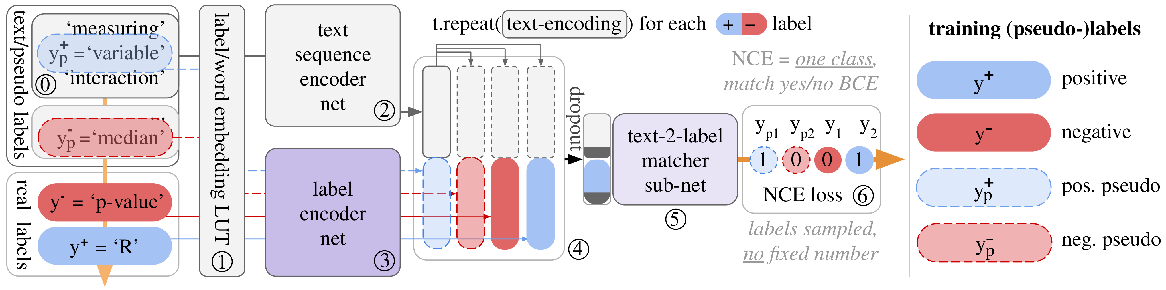
As done in natural language usage, we express labels as words, or more specifically as word embeddings, rather than as label vectors. CLESS then learns to contrastively (mis-)match <text embedding, (pseudo/real) label embedding> pairs as overviewed in Figure 1. For self-supervised pretraining, we in-batch sample g (good) positive and b (bad) negative <text, pseudo label> embedding pairs per text instance to then learn good and bad matches from them. Positive pseudo labels are a sampled subset of words that appear in the current text instance. Negative pseudo labels are words sampled from the other texts within a batch. Crucially, negative words (pseudo labels) can not be the same words as positive words (pseudo labels)—i.e. .
This deceptively simple sampling strategy ensures that we fulfill two important criteria for successful self-supervised contrastive learning. One, using multiple positive labels improves learning if we draw them from a similar (related) context, as Wang and Isola [25] proved. Two, we avoid collisions between positive and negative samples, which otherwise degrades learning when using more negatives as Saunshi et al. [22] find. Similarly, for supervised learning, we use g positive, real labels and undersample b negative labels to construct <text, positive/negative real label> pairs. A text-2-label classifier ➄ learns to match <text, label> embedding pairs using a noise contrastive loss [35], which we extend to use g positives rather than just one. This unifies self-supervised and supervised learning as contrastive ‘text embedding to (label) text embedding matching’ and allows direct transfer like zero-shot predictions of real labels after pseudo label pretraining—i.e. without prior training on other real labels as required by methods like [15,19,36]. Below, we describe our approach and link specific design choices to insights from existing research in steps ➀–➅.
We give the model a text instance i of words and a set of positive and negative label words . We also construct a label indicator as ground truth labels for the binary NCE loss in ➅. This label indicator contains a g-sized vector of ones to indicate positive (matching) <text, label> embedding pairs and a b-sized zero vector to indicated mismatching pairs, resulting in the indicator
CLESS then encodes input text and labels in three steps ➀–➂. First, both the input text (words) and the labels are passed through a shared embedding layer ➀ to produce as text embeddings and as label embeddings. Then, the text embeddings are encoded via a text encoder T ➁, while labels are encoded by a label encoder L as follows:
To make model learning more data-efficient we initialize the embedding layer E with fastText word embeddings that we train on the 60MB of in-domain text data. Such word embedding training only computes a few seconds, while enabling one to make the text encoder architecture small, but well initialized. The text encoder T consists of a single, k-max-pooled CNN layer followed by a fully connected layer for computation speed and data-efficiency [30,37,38]. As a label encoder L, we average the embeddings of words in a label and feed them through a fully connected layer—e.g. to encode a label ‘p-value’ we simply calculate the mean word embedding for the words ‘p’ and ‘value’.
To learn whether a text instance embedding matches any of the c label embeddings , we repeat the text embedding , c times, and concatenate text and label embeddings to get a matrix of <text, label> embedding pairs:
This text-label paring matrix is then passed to the matcher network M ➄, which first applies dropout to each text-label embedding pair and then uses a three layer MLP to produce a batch of c label match probabilities:
Here, applying dropout to label and text embeddings induces a dense version of label noise. Discrete {0,1} label dropout has been shown to improve robustness to label noise in Szegedy et al. [33], Lukasik et al. [39]. Because we always predict correct pseudo labels in pretraining, this forces the classifier to learn to correct dropout induced label noise.
Finally, we use a binary noise contrastive estimation loss as in [35], but extend it to use g positives, not one.
Here, is the mean binary cross-entropy loss of g positive and b negative labels—i.e. it predicts label probabilities , where the label indicators from ➀ are used as ground truth labels.
Though we focus on evaluating CLESS for long-tail prediction in this work, other NLP tasks such as question answering or recognizing textual entailment can similarly be modeled as contrast pairs . Unlike T5 language models [16], this avoids translating back and forth between discrete words and dense token embeddings. Not using T5s’ softmax objective, also allows for predicting unforeseen (unlimited) test classes (label). We provide details on hyperparameter tuning of CLESS for self-supervised and supervised learning in Appendix C.
4. Data: Resource Constrained, Long-Tail, Multi-Label, Tag Prediction
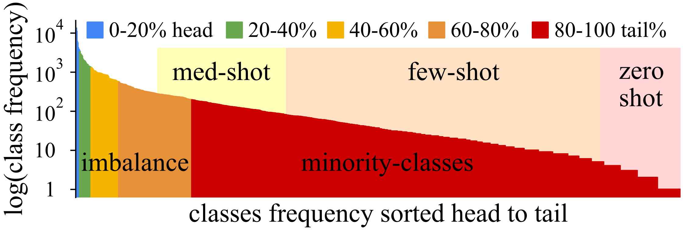
To study efficient, small model, long-tail learning for ‘text-to-text’ pretraining models, we choose a multi-label question tag prediction dataset as a testbed. We use the “Questions from Cross Validated” dataset, where machine learning concepts are tagged per question—https://www.kaggle.com/stackoverflow/statsquestions, accessed on 30 August 2021. This dataset is small (80MB of text), and entails solving a challenging ‘text-to-text’ long-tailed prediction task. The dataset has 85k questions with 244k positive labels, while we do not use answer texts. As with many real-world problems, labels are vague, since tagging was crowd-sourced. This means that determining the correct amount of tags per question (label density) is hard, even for humans. The task currently has no prior state-of-the-art. As seen in Figure 2, the datasets’ class occurrence frequencies are highly long-tailed, i.e. the 20% most frequently occurring classes result in 7 ‘head’ classes, while the 20% least frequent (rightmost) label occurrences cover 80% or 1061/1315 of classes. Tags are highly sparse—at most 4 out of 1315 tags are labeled per question. We pretrain fastText word embeddings on the unlabeled text data to increase learning efficiency, and because fastText embeddings only take a few seconds to pretrain. The full details regarding preprocessing can be found in Appendix A.
- Long-tail evaluation metrics and challenges:
Long-tail, multi-label classification is challenging to evaluate because (i) top-k quality measures mask performance losses on long-tailed minority classes as Hooker et al. [6] point out. Furthermore, (ii) measures like overestimate performance under class imbalance [40,41], and (iii) discrete measures like F-score are not scalable, as they require discretization threshold search under class imbalance. Fortunately, the Average Precision score addresses issues (i-iii), where and are precision and recall at the nth threshold. We choose weighting as this score variant is the hardest to improve.
5. Results
In this section, we analyze the three research questions: (RQ-1) Does RoBERTa learn long-tail tag prediction well? (RQ-2) Can a 12.5× smaller CLESS model achieve good long-tail prediction, and at what cost? (RQ-3) How does CLESS compare in zero to few-shot prediction and does its model size matter. We split the dataset into 80/10/10 for training, development, and test set. Test scores or curves are reported for models that have the best development set average precision score over all 1315 classes. RoBERTa has 125 million parameters and is pretrained on 160GB of text data. CLESS has 8-10 million parameters and is pretrained on just 60MB of in-domain text data. We use a ZeroR classifier, i.e. predicting the majority label per class, to establish imbalanced guessing performance. The ZeroR on this dataset is since a maximum of 4 in 1315 classes are active per instance—i.e., which underlines the challenge of the task.
5.1. (RQ-1+2): Long-Tail Capture of RoBERTa vs. CLESS
Here we compare the long-tail prediction performance of RoBERTa (1) vs. CLESS setups that, either were pretrained (3, 3.XL), or not pretrained (2). Plotting individual scores for 1315 classes is unreadable. Instead, we sort classes from frequent to rare and assign them to one of five ‘ of the overall class frequency’ bins, such that all bins are balanced. This means all bins contain the same amount of positive real labels (label occurrences) and are directly comparable. As seen in Figure 2, this means that the head bin (left) contains the most frequent classes, while the tail contains the most rarely occurring classes.
5.1.1. RoBERTa: A Large Pretrained Model Does Not Guarantee Long-Tail Capture
Figure 3 shows how a tag prediction fine-tuned RoBERTa performs over the five class bins as described above or in Section 4. RoBERTa learns the most common ( head) classes well, but struggles with mid to tail classes. On the tail class bin, i.e., on of classes, RoBERTa performs worse than a CLESS model that did not use contrastive pretraining (2). This allows multiple insights. One, a large PLM should not implicitly be assumed to learn long-tail information well. Two, large-scale pretraining data should not be expected to contain enough (rare) long-tailed domain information for an arbitrary end-task, since in the tail-domain, data is always limited. Three, even a small supervised contrastive model, without pretraining, can improve long-tail retention (for 80.7% of classes). Together these results indicate that compressing a large PLM may not be the optimal approach to training a small, long-tail prediction capable model.
5.1.2. CLESS: Contrastive Pretraining Removes the Need for Model Compression
Model (3) and (3.XL) use our contrastive pretraining on the end-tasks’ 60MB of unlabeled text data before supervised fine-tuning. We see that models with contrastive pretraining (3, 3.XL) noticeably outperform RoBERTa (1) and the non-pretrained contrastive model (2), on all non-head class bins, but especially on the tail classes. We also see that the pretraining model parameter amount impacts CLESS performance as the 10 million parameter model (3.XL) outperforms the 8M parameters model (3) over all class bins and especially the tail bin. The above observations are especially encouraging as they tell us that contrastive in-domain pretraining can produce small, long-tail learning capable models without the need for compressing large models. It also tells us that model capacity matters in long-tail information retention, but not in the common sense that large PLMs are as useful as they have proven to be for non-long-tail learning applications. This also means that contrastive self-supervised LM pretraining can help reduce algorithmic bias caused by long-tail information loss in smaller models, the potential fairness impact of which was described by [1,2,6].
5.1.3. Practical Computational Efficiency of Contrastive Language Modeling
Though the long-tail performance results of CLESS are encouraging, its computational burden should ideally be equal or less than that of fine-tuning RoBERTa. When we analyzed training times we found that RoBERTa took 126 GPU hours to fine-tune for 48 epochs, when using 100% of fine-tuning labels. For the same task we found that CLESS (3.XL) took 7 GPU hours for self-supervised pretraining (without labels) and 5 GPU hours for supervised fine-tuning over 51 epochs—To bring CLESS to the same GPU compute load as RoBERTa (%) we parallelized our data generation—otherwise our training times double and the GPU load is only %. As a result, pretraining plus fine-tuning takes CLESS (3.XL) 12 h compared to 126 for fine-tuning RoBERTa. This means that the proposed contrastive in-domain pretraining has both qualitative and computational advantages, while remaining applicable in scenarios where large collections of pretraining data are not available—which may benefit use cases like non-English or medical NLP. Additionally, both methods benefit from parameter search, but since CLESS unifies self-supervised pretraining and supervised fine-tuning as one objective we can reuse pretraining hyperparameters during fine-tuning. A more in-depth account of computational trade-offs is given in Appendix B, while details of hyperparameter tuning are given in Appendix C.
It is of course possible to attempt to improve the long-tail performance of RoBERTa, e.g. via continued pretraining on the in-domain data [42] or by adding new tokens [43,44]. However, this further increases the computation and memory requirements of RoBERTa, while the model still has to be compressed—which requires even more computation. We also tried to further improve the embedding initialization of CLESS using the method described in [45], to further boost its learning speed. While this helped learning very small models (M parameters), it did not meaningfully impact the performance of contrastive pretraining or fine-tuning.
5.2. (RQ-3.1-2): Contrastive Zero-Shot Long-Tail Learning
Thanks to the unified learning objective for self-supervised and supervised learning, CLESS enables zero-shot prediction of long-tail labels after self-supervised pretraining, i.e. without prior training on any labels. Therefore, in this section, we analyze the impact of using more model parameters (RQ-3.1) as well as using more pseudo labels (RQ-3.2) during self-supervised contrastive pretraining.
5.2.1. (RQ-3.1): More Self-supervision and Model Size Improve Zero-Shot Long-Tail Capture
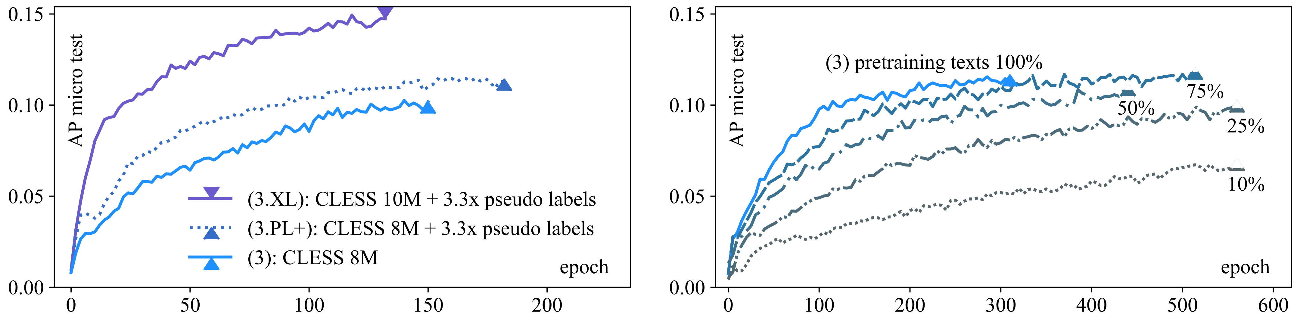
In Section 4, we study how CLESSs’ zero-shot long-tail retention ability is impacted by: (left) using more pseudo labels (learning signal) during pretraining; and (right) by using only portions of unlabeled text data for pretraining. To do so, we pretrain CLESS variants on pseudo labels and evaluate each variant’s zero-shot performance over all 1315 classes of the real-label test set from Section 4. As before, we show test score curves for the models with the best dev set performance.
The left plot of Figure 4, shows the effect of increasing the number of self-supervision pseudo label and model parameters. The CLESS 8M model (3), pretrained with 8 million parameters and 150 pseudo labels, achieves around on the test real labels as zero-shot long-tail performance. When increasing the pseudo label number to 500 in model (3.PL+), the model gains zero-shot performance (middle curve), without requiring more parameters. When additionally increasing the model parameters to 10M in (3.XL), the zero-shot performance increases substantially (top curve). Thus, both increasing self-supervision signal amount and model size boost zero-shot performance.
5.2.2. RQ-3.2: Contrastive pretraining Leads to Data-Efficient Zero-Shot Long-Tail Learning
Further, in the right plot of Figure 4 we see the CLESS 8M model (3) when trained on increasingly smaller portions () of pretraining text. For all but the smallest pretraining data portions () the model still converges towards the original 100% performance. However, as expected, its convergence slows proportionally with smaller pretraining text portions since each data reduction implies seeing less pseudo label self-supervision per epoch. As a result, the data reduced setups need more training epochs, so we allowed more waiting-epochs for early stopping than in the left plot. Thus, our contrastive self-supervised objective can pretrain data-effectively from very limited data. Similar data-efficiency gains from using contrastive objectives were previously only observed in computer vision applications by Zimmermann et al. [18], which confirms our initial intuition that contrastive self-supervision is generally useful for self-supervised learning from limited data.
Methods like Pappas and Henderson [15], Jiang et al. [36], Augenstein et al. [46] required supervised pretraining on real labels to later predict other, unseen labels in a zero-shot fashion. CLESS instead uses self-supervised pretraining to enable zero-shot prediction without training on real labels. This ‘text-to-text’ prediction approach is intentionally reminiscent of zero-shot prediction approaches in large PLMs like GPT-3 [47], but is instead designed to maximize zero-shot, long-tail prediction for use cases that strongly limit pretraining data amounts and model size. Hooker et al. [6] hypothesized that long-tail prediction depends on the model capacity (parameter amount). Additionally, Brown et al. [47] found that zero-shot prediction performance depends on model capacity, but [48,49] experimentally showed or visualized how inefficiently model capacity is used by common models, especially after fine-tuning. From the above observations, we can confirm the impact of model size for the doubly challenging task of long-tail, zero-shot prediction, but we can also confirm that contrastive pretraining allows a model to much more efficiently use its capacity for long-tail capture, i.e., requiring 12.5x fewer parameters (capacity) than common the RoBERTa model. Perhaps more encouragingly, we also observed that cheap, contrastive in-domain pretraining boosts zero-shot prediction, even when pretraining data is very limited—i.e. either by lack of large domain text data or due to data limitations caused by a long-tail distribution.
5.3. (RQ-3.3): Few-Shot Long-Tail Learning
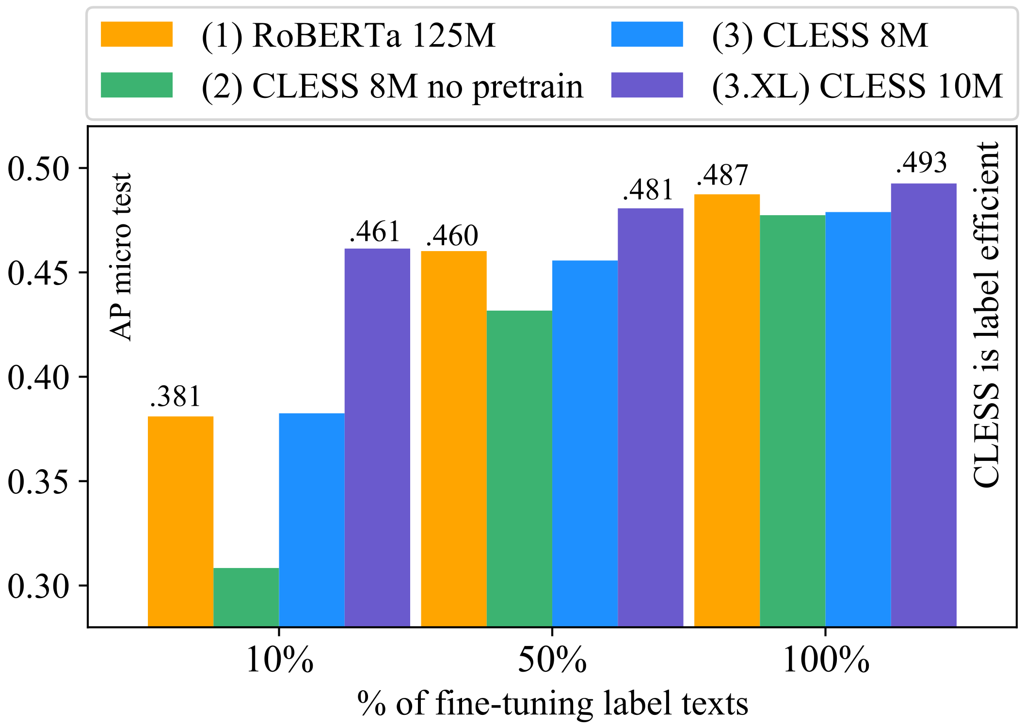
Since CLESS models allow direct transfer (reuse) of the pretrained prediction head for supervised label prediction one would also expect the models’ few-shot long-tail prediction performance to benefit from self-supervised pretraining. We thus study the few-shot learning performances of both CLESS and RoBERTa, to understand differences in large pretrained language models (PLMs) and small contrastive language model (CLM) pretraining in more detail. For the few-shot setup, we use 100%, 50% and 10% of labeled text instances for supervised training or fine-tuning of all models. This implies that if labels were common in the 100% setup, they now become increasingly rare or few-shot in the 10% setup, since the smaller label sets are still long-tail distributed. We again use test set performance over all 1315 classes to compare models.
In Figure 5, we see that when using full supervision (100%), all models perform similarly, with CLESS (3.XL) slightly outperforming RoBERTa (0.493 vs. 0.487) . For few-shot learning (10%, 50%), we see that CLESS 3.XL retrains of its original performance when using only 10% of fine-tuning labels, while RoBERTa and CLESS 8M each retain around 77%. This demonstrates that even a sightly larger contrastive pretraining model, with increased self-supervision signal (3.XL), not only improves zero-shot learning performance as was seen in Figure 4, but also markedly boosts few-shot performance. Noticeably, the only non-pretrained model (2), performs much worse than the others in the more restricted few-shot scenarios. Since models (2) and (3) use the same hyperparameters and only differ in being pretrained (3) or not being pretrained (2), this demonstrates that contrastive self-supervised pretraining largely improves label efficient learning.
6. Conclusion
We introduce CLESS, a contrastive self-supervised language model (CLM), that unifies self-supervised pretraining and supervised fine-tuning into a single contrastive ‘text embedding to text embedding’ matching objective. Through three research questions (RQ-1 to RQ-3) we demonstrate that this model learns superior zero-shot, few-shot, and fully supervised long-tail retention in small models without needing to compress large models. In RQ-1, we first show that a fine-tuned, large pretrained language model like RoBERTa should not implicitly be expected to learn long-tail information well. Then, in RQ-2, we demonstrate that our contrastive self-supervised pretraining objective enables very text data-efficient pretraining, which also results in markedly improved (label efficient) few-shot or zero-shot long-tail learning. Finally, in RQ-3, we find that using more contrastive self-supervision signals and increasing model parameter capacity play important roles in boosting zero to few-shot long-tail prediction performance when learning from very limited in-domain pretraining data. We also find that the very low compute requirements of our method make it a viable alternative to large pretrained language models, especially for learning from limited data or in long-tail learning scenarios, where tail data is naturally limited. In future work, we envision applying CLESS to low-data domains like medicine [27] and fact-checking [50], or to tasks where new labels emerge at test time, e.g. hashtag prediction [51]. Code and setup can be found at https://github.com/NilsRethmeier/CLESS (accessed on 30 August 2021).
Author Contributions
Conceptualization, N.R., I.A.; methodology, N.R.; software, N.R.; validation, N.R., I.A.; formal analysis, N.R., I.A.; investigation, N.R.; resources, N.R.; data curation, N.R.; writing—original draft preparation, N.R., I.A.; writing—review and editing, N.R., I.A.; visualization, N.R.; supervision, I.A.; project administration, N.R., I.A.; funding acquisition, N.R., I.A. All authors have read and agreed to the published version of the manuscript.
Funding
This research was conducted within the Cora4NLP project, which is funded by the German Federal Ministry of Education and Research (BMBF) under funding code 01IW20010.
Institutional Review Board Statement
Not applicable.
Informed Consent Statement
Not applicable.
Data Availability Statement
The dataset used in this study can be found as described in the data section. The exact training data setup is available online and upon request to the corresponding author.
Acknowledgments
We thank Yanai Elazar, Pepa Atanasova, Christoph Alt, Leonard Hennig and Dustin Wright for providing feedback and discussion on earlier drafts of this work.
Conflicts of Interest
The authors declare no conflict of interest.
Appendix A
Text preprocessing details: We decompose tags such as ‘p-value’ as ‘p’ and ‘value’ and split latex equations into command words, as they would otherwise create many long, unique tokens. In the future, character encodings may be better for this specific dataset, but that is out of our current research scope. Words embedding are pretrained via fastText on the training corpus text. 10 tag words are not in the input vocabulary and thus we randomly initialize their embeddings. Though we never explicitly used this information, we parsed the text and title and annotated them with ‘Html-like’ title, paragraph, and sentence delimiters, i.e. </title>, </p>, and </s>.
Appendix B
Here we will discuss the time and transfer complexity of CLESS vs. Self-attention models. We do so since time complexity is only meaningful if the data-efficiency of two methods is the same, because the combination of convergence speed, computation speed, and end-task performance makes a model effective and efficient.

Table A1.
Time complexity O(Layer), data-efficiency, number of trainable parameters, number of all parameters. The data-efficiency of Convolutions (*) is reported in various works to be superior to that of self-attention models [28,30,52,53,54,55,56]. d is the input embedding size and its increase slows down convolutions. n is the input sequence length and slows down self-attention the most [57]. There exist optimizations for both problems.
| Layer Type | Literature Reported Data Requirements | Trainable Parameters | |
| Convolution | small (*) | 8M-10M (CLESS) | |
| Self-Attention | large to web-scale (*) | 125M (RoBERTa) |
Time complexity: Our text encoder uses a single 1D CNN encoder layer which has a complexity of vs. for vanilla self-attention as outlined in Vaswani et al. [57]. Here n is the input sequence length, k is the convolution filter size, d is the input embedding dimension [ in [57] vs. for us], and f is the number of convolution filters (at maximum for our (3.XL) pretraining model). Since we use kernel sizes we get for the largest configuration (3.XL) an vs. in a vanilla (2017) self-attention setup where d = 512. Furthermore Transformer self-attention runs an n-way soft-max computation at every layer (e.g. 16 layers), while we run single-class predictions at the final output layer using a noise contrastive objective NCE. We use NCE to undersample both: true negative learning labels (label=0) as well as positive and negative pseudo labels (input words). If the goal is to learn a specific supervised end-task, more informed sampling of positive and negative pseudo labels can be devised. However, we did not intend to overfit the supervised task by adding such hand-crafted human biases. Instead we use random sampling to pretrain a model for arbitrary downstream tasks (generalization), which follows a similar logic as random masking does in masked language modeling.
Transfer complexity: Traditional transfer NLP approaches like RoBERTa [13] need to initialize a new classification head per task which requires either training a new model per task or a joint multi-task learning setup. CLESS however can train multiple tasks, even if they arrive sequentially over time, while reusing the same classifier head from prior pretraining or fine-tuning. Thus, there is no need to retrain a separate model each time as in current Transformer transfer models. Once pretrained a CLESS model can zero-shot transfer to any new task since the match classifier is reused.
Appendix C
In this section, we describe the data and memory efficiency of the proposed method as well as the hyperparameter tuning we conducted.
Data, sample and memory efficiency: We analyzed input data and label efficiency in the main documents zero and few-shot learning sections. Regarding data-efficiency and model design choices we were guided by the existing research and optimized for data-efficient learning with inherent self-supervised zero-shot capabilities in order to facilitate and study supervision-free generalization to unforeseen tasks. We explain the origins of these design choices in more detail below. As mentioned in the related research section, Transformers rely on large to Web-scale pretraining data collections ‘end-task external pretraining data’ [52,53], which results in extensive pretraining hardware resources [58,59], concerns about environmental costs [56,60] and unintended contra-minority biases [56,61,62]. CNNs have been found to be more data-efficient than Transformers, i.e., train to better performance with less data, several works. For example in OPENAI’s CLIP model, see Figure 2 in [30], the authors find that replacing a Transformer language model backbone with a CNN backbone increased the zero-shot data-efficiency 3 fold, which they further increased by adding a supervised contrastive learning objective. [38] showed that adding a CNN component to a vision Transformer model helps with data and computational efficiency, see Figure 5 and text in [38]. When comparing works on small-scale data pretraining capabilities between [54] (CNN, LSTM) with recent Transformer models Wang et al. [55], one can see that Transformer encoders struggle to learn from small pretraining collections. They also struggle to fine-tuning on smaller supervised collections [12,32,59]. For CLESS, tuning the embedding layer made little difference to end-task performance, when starting training with pretrained fastText word embedding. Thus embedding tuning the embedding layer can be turned off to reduce gradient computation and memory. For example, when not tuning embeddings, the CLESS 10M model has only 3.2M trainable parameters.
Table A2.
Explored parameters. We conducted a random grid search over the following hyperparameters while optimizing important parameters first to largely limit trials. We also pre-fit the filter size, lr, and filters on a 5k training subset of samples to further reduce trails. Then, to further reduce the number of trials, we tuned in the following order: learning rate , filter sizes f, max-k pooling, tuning embeddings, batch size , and finally the depth of the matching-classifier MLP. This gave us a baseline model, (2) CLESS 8M, that does not use pretraining to save trials and compute costs, but could be used to build up into the self-supervised pretraining models (3) and (3.XL) by increasing self-supervision and model size. Fortunately, RoBERTa has established default parameters reported in both its code documentation (https://github.com/pytorch/fairseq/tree/master/examples/roberta) (accessed on 30 September 2021) and the https://simpletransformers.ai (accessed on 30 September 2021) version, where we varied batch size, warmup, and learning rate around the default setting of these sources. Below we give the search parameters for CLESS. For CLESS 8M (2,3) the best params are italic and for CLESS 10M (3.XL) the best params are bold.
| Filter size: num filters | {1: 57, 2: 29, 3: 14}, {1:100, 2:100, 1:100},{1: 285, 2: 145, 3: 70}, {1:10, 10:10, 1:10}, {1:15, 2:10, 3:5}, {1:10}, {1:100}, {10:100} |
| lr | 0.01, 0.0075, 0.005, 0.001, 0.0005, 0.0001 |
| bs (match size) | 1024, 1536, 4096 |
| max-k | 1, 3, 7, 10 |
| match-classifier | two_layer_classifier, ’conf’:[{’do’: None|.2, ’out_dim’: 2048|4196|1024}, {’do’:None|0.2}]}, one_layer_classifier, ’conf’:[{’do’:.2}]} |
| label encoder | one_layer_label_enc, ’conf’:[{’do’:None|.2, ’out_dim’: 100}, one_layer_label_enc, ’conf’:[{’do’: .2, ’out_dim’: 300} |
| seq encoder | one_layer_label_enc, ’conf’:[{’do’:None|.2, ’out_dim’: 100}, one_layer_label_enc, ’conf’:[{’do’: .2, ’out_dim’: 300} |
| tune embedding: | True, False |
| #real label samples: | 20, 150, 500 (g positives (as annotated in dataset), b random negative labels—20 works well too) |
| #pseudo label samples: | 20, 150, 500 (g positives input words, b negative input words)—used for self-superv. pretraining |
| optimizer: | ADAM—default params, except lr |
Parameter tuning + optima (2)-(3.XL) We provide detailed parameter configurations as python dictionaries for reproducibility in the code repository within the /confs folder. In Table A2 we see how the hyperparameters explored in CLESS—the optimal CLESS 3.XL parameters are marked in bold. The baseline CLESS configuration (2) hyperparameters were found as explained in the table, using the non-pretraining CLESS 8M (2) model—its best parameters are italic. We found these models by exploring hyperparameters that have been demonstrated to increase generalization and performance in [63,64]. To find optimal hyperparameter configurations for the baseline model (2) we ran a random grid search over the hyperparameter values seen in Table A2. For the baseline CLESS 8M model (2), without pretraining, we found optimal hyperparameters to be: (lr=0.0005 works too), , =two_layer_classifier, ’conf’:[{’do’: None|.2, ’out_dim’: 2048 | 4196 | 1024}, =7, =1536, etc.—see Table A2. Increasing the filter size, classifier size, its depth, or using larger k in k-max pooling decreased dev set performance of the non-pretrained model (i.e., CLESS 8M) due to increased overfitting. The largest pretrained CLESS 10M (3.XL) model was able to use more: ‘max-k=10’, a larger ‘label’ and ‘text sequence encoder’= one_layer_label_enc, ’conf’:[{’do’: .2, ’out_dim’: 300} while the batch size shrinks to 1024 due to increased memory requirements of label matching. Note that label and text encoder have the same output dimension in all settings—so text and label embeddings remain in the same representation dimensionality . The label encoder averages word embeddings (average pooling), while the text encoder uses a CNN with filters as in Table A2. The model receives text word ids and label-word ids, that are fed to the ‘text encoder’ and ‘label-encoder’. These encoders are sub-networks that are configured via dictionaries to have fully connected layers and dropout, with optimal configurations seen in the table. As the match-classifier, which learns to contrast the (text embedding, label embedding) pairs, we use a which learns a similarity (match) function between text embedding to label embedding combinations (concatenations).
During self-supervised pretraining, the models (3) and (3.XL) optimize for arbitrary unforeseen long-tail end-tasks, which allows zero-shot prediction without ever seeing real labels, but also uses a very diverse learning signal by predicting sampled positive and negative input word embeddings. If the goal is to solely optimize for a specific end-task, this self-supervision signal can be optimized to pretrain much faster, e.g. by only sampling specific word types like nouns or named entities. With specific end-task semantics in mind, the pseudo label and input manipulations can easily be adjusted. This allows adding new self-supervision signals without a need to touch the model’s network code directly, which helps ease application to new tasks and for less experienced machine learning practitioners. Finally, we mention implementation features, that can safely be avoided to reduce computation and optimization effort, so that following research needs not explore this option. When training the supervised and self-supervised loss at the same time (jointly), CLESS rescales both batch losses to be of the same loss value as using a single loss. This makes it easy to balance (weight) the two loss contributions in learning, and allows transferring hyperparameters between self-supervised and supervised pretraining. We also allow re-weighting the loss balance by a percentage, so that one loss can dominate. However, we found that in practice: (a) using the self-supervised loss along with the supervised one does not improve quality, but slows computation (2 losses). (b) We also found that, if one decides to use joint self and supervised training, loss re-weighting had no marked quality effects, and should be left at 1.0 (equal weighting), especially since it otherwise introduces further, unnecessary hyperparameters. For pretraining research, hyperparameter search is very involved, because we deviate in common practice by introducing a new architecture, a new loss variation, an uncommon optimization goal and metrics as well as a new dataset. Thus we ended up with 205 trails for small test set, RoBERTa, CLESS variants, zero-shot and few shot hyperparameter search. On the herein reported dataset, we have not yet tested further scaling up model parameters for pretraining as this goes against the goal of the paper and is instead investigated in followup work. Furthermore, when we ran such parameter scale-up experiments, to guarantee empirical insights, these created a significant portion of trails, meaning that, now that sensible parameters are established, we can use much fewer trials, as is the case with pretrained transformers. The work at hand suggest that, once sensible parameters are established, they are quite robust, such that doubling the learning rate, batch size and loss weighting only cause moderate performance fluctuations. Finally, the above reported pretraining hyperparameters seem to work well on currently developed followup research, that uses other, even much larger, datasets. This makes the 205 hyperparameter trials a one time investment for initial pretraining hyperparameter (re)search for this contrastive language model (CLESS).
References
- Hooker, S.; Courville, A.; Clark, G.; Dauphin, Y.; Frome, A. What Do Compressed Deep Neural Networks Forget? arXiv 2020, arXiv:1911.05248. [Google Scholar]
- Hooker, S. Moving beyond “algorithmic bias is a data problem”. Patterns 2021, 2, 100241. [Google Scholar] [CrossRef] [PubMed]
- Liu, Z.; Miao, Z.; Zhan, X.; Wang, J.; Gong, B.; Yu, S.X. Large-Scale Long-Tailed Recognition in an Open World. In Proceedings of the IEEE CVPR, Long Beach, CA, USA, 16–20 June 2019; pp. 2537–2546. [Google Scholar] [CrossRef] [Green Version]
- D’souza, D.; Nussbaum, Z.; Agarwal, C.; Hooker, S. A Tale of Two Long Tails. arXiv 2021, arXiv:2107.13098. [Google Scholar]
- Hu, N.T.; Hu, X.; Liu, R.; Hooker, S.; Yosinski, J. When does loss-based prioritization fail? arXiv 2021, arXiv:2107.07741. [Google Scholar]
- Hooker, S.; Moorosi, N.; Clark, G.; Bengio, S.; Denton, E. Characterizing and Mitigating Bias in Compact Models. In Proceedings of the 5th ICML Workshop on Human Interpretability in Machine Learning (WHI), Virtual Conference, 17 July 2020. [Google Scholar]
- Zhuang, D.; Zhang, X.; Song, S.L.; Hooker, S. Randomness In Neural Network Training: Characterizing The Impact of Tooling. arXiv 2021, arXiv:2106.11872. [Google Scholar]
- Chang, W.C.; Yu, H.F.; Zhong, K.; Yang, Y.; Dhillon, I. X-BERT: eXtreme Multi-label Text Classification with using Bidirectional Encoder Representations from Transformers. arXiv 2019, arXiv:1905.02331. [Google Scholar]
- Joseph, V.; Siddiqui, S.A.; Bhaskara, A.; Gopalakrishnan, G.; Muralidharan, S.; Garland, M.; Ahmed, S.; Dengel, A. Reliable model compression via label-preservation-aware loss functions. arXiv 2020, arXiv:2012.01604. [Google Scholar]
- Blakeney, C.; Huish, N.; Yan, Y.; Zong, Z. Simon Says: Evaluating and Mitigating Bias in Pruned Neural Networks with Knowledge Distillation. arXiv 2021, arXiv:2106.07849. [Google Scholar]
- Jiang, Z.; Chen, T.; Mortazavi, B.J.; Wang, Z. Self-Damaging Contrastive Learning. Proc. Mach. Learn. Res. PMLR 2021, 139, 4927–4939. [Google Scholar]
- Rogers, A.; Kovaleva, O.; Rumshisky, A. A Primer in BERTology: What We Know About How BERT Works. Trans. Assoc. Comput. Linguist. 2020, 8, 842–866. [Google Scholar] [CrossRef]
- Liu, Y.; Ott, M.; Goyal, N.; Du, J.; Joshi, M.; Chen, D.; Levy, O.; Lewis, M.; Zettlemoyer, L.; Stoyanov, V. RoBERTa: A Robustly Optimized BERT Pretraining Approach. arXiv 2019, arXiv:1907.11692. [Google Scholar]
- Liu, J.; Chang, W.; Wu, Y.; Yang, Y. Deep Learning for Extreme Multi-label Text Classification. In Proceedings of the 40th International ACM SIGIR Conference on Research and Development in Information Retrieval, Shinjuku, Tokyo, Japan, 7–11 August 2017; pp. 115–124. [Google Scholar] [CrossRef]
- Pappas, N.; Henderson, J. GILE: A Generalized Input-Label Embedding for Text Classification. Trans. Assoc. Comput. Linguistics 2019, 7, 139–155. [Google Scholar] [CrossRef]
- Raffel, C.; Shazeer, N.; Roberts, A.; Lee, K.; Narang, S.; Matena, M.; Zhou, Y.; Li, W.; Liu, P.J. Exploring the Limits of Transfer Learning with a Unified Text-to-Text Transformer. J. Mach. Learn. Res. 2020, 21, 1–67. [Google Scholar]
- Graf, F.; Hofer, C.; Niethammer, M.; Kwitt, R. Dissecting Supervised Constrastive Learning. Proc. Mach. Learn. Res. PMLR 2021, 139, 3821–3830. [Google Scholar]
- Zimmermann, R.S.; Sharma, Y.; Schneider, S.; Bethge, M.; Brendel, W. Contrastive Learning Inverts the Data Generating Process. Proc. Mach. Learn. Res. PMLR 2021, 139, 12979–12990. [Google Scholar]
- Zhang, H.; Xiao, L.; Chen, W.; Wang, Y.; Jin, Y. Multi-Task Label Embedding for Text Classification. In Proceedings of the 2018 Conference on Empirical Methods in Natural Language Processing, Brussels, Belgium, 2–4 November 2018; Association for Computational Linguistics: Stroudsburg, PA, USA, 2018; pp. 4545–4553. [Google Scholar] [CrossRef] [Green Version]
- Musgrave, K.; Belongie, S.J.; Lim, S. A Metric Learning Reality Check. In Proceedings of the Computer Vision-ECCV 2020-16th European Conference, Glasgow, UK, 23–28 August 2020; pp. 681–699. [Google Scholar] [CrossRef]
- Rethmeier, N.; Augenstein, I. A Primer on Contrastive Pretraining in Language Processing: Methods, Lessons Learned and Perspectives. arXiv 2021, arXiv:2102.12982. [Google Scholar]
- Saunshi, N.; Plevrakis, O.; Arora, S.; Khodak, M.; Khandeparkar, H. A Theoretical Analysis of Contrastive Unsupervised Representation Learning. Proc. Mach. Learn. Res. PMLR 2019, 97, 5628–5637. [Google Scholar]
- Khosla, P.; Teterwak, P.; Wang, C.; Sarna, A.; Tian, Y.; Isola, P.; Maschinot, A.; Liu, C.; Krishnan, D. Supervised Contrastive Learning. In Advances in Neural Information Processing Systems 33 (NeurIPS 2020); Larochelle, H., Ranzato, M., Hadsell, R., Balcan, M.F., Lin, H., Eds.; Curran Associates, Inc.: Red Hook, NY, USA, 2020; Volume 33, pp. 18661–18673. [Google Scholar]
- Ostendorff, M.; Rethmeier, N.; Augenstein, I.; Gipp, B.; Rehm, G. Neighborhood Contrastive Learning for Scientific Document Representations with Citation Embeddings. arXiv 2022, arXiv:2202.06671. [Google Scholar]
- Wang, T.; Isola, P. Understanding Contrastive Representation Learning through Alignment and Uniformity on the Hypersphere. Proc. Mach. Learn. Res. PMLR 2020, 119, 9929–9939. [Google Scholar]
- Mnih, A.; Teh, Y.W. A Fast and Simple Algorithm for Training Neural Probabilistic Language Models. In Proceedings of the 29th International Conference on International Conference on Machine Learning (ICML’12), Edinburgh, UK, 26 June–1 July 2012; Omnipress: Madison, WI, USA; pp. 419–426. [Google Scholar]
- Şerbetci, O.N.; Möller, S.; Roller, R.; Rethmeier, N. EffiCare: Better Prognostic Models via Resource-Efficient Health Embeddings. AMIA Annu. Symp. Proc. 2020, 2020, 1060–1069. [Google Scholar]
- Kim, K.M.; Hyeon, B.; Kim, Y.; Park, J.H.; Lee, S. Multi-pretraining for Large-scale Text Classification. In Findings of the Association for Computational Linguistics: EMNLP 2020; Cohn, T., He, Y., Liu, Y., Eds.; Association for Computational Linguistics: Stroudsburg, PA, USA, 2020; pp. 2041–2050. [Google Scholar] [CrossRef]
- Tay, Y.; Dehghani, M.; Gupta, J.; Bahri, D.; Aribandi, V.; Qin, Z.; Metzler, D. Are Pre-trained Convolutions Better than Pre-trained Transformers? arXiv 2021, arXiv:2105.03322. [Google Scholar]
- Radford, A.; Kim, J.W.; Hallacy, C.; Ramesh, A.; Goh, G.; Agarwal, S.; Sastry, G.; Askell, A.; Mishkin, P.; Clark, J.; et al. Learning Transferable Visual Models From Natural Language Supervision. Proc. Mach. Learn. Res. PMLR 2021, 139, 8748–8763. [Google Scholar]
- Devlin, J.; Chang, M.; Lee, K.; Toutanova, K. BERT: Pre-training of Deep Bidirectional Transformers for Language Understanding. Proceedings of NAACL-HLT 2019, Minneapolis, MN, USA, 2–7 June 2019; Association for Computational Linguistics: Stroudsburg, PA, USA, 2019; pp. 4171–4186. [Google Scholar] [CrossRef]
- Liu, L.; Liu, X.; Gao, J.; Chen, W.; Han, J. Understanding the Difficulty of Training Transformers. arXiv 2020, arXiv:2004.08249. [Google Scholar]
- Szegedy, C.; Vanhoucke, V.; Ioffe, S.; Shlens, J.; Wojna, Z. Rethinking the Inception Architecture for Computer Vision. In Proceedings of the 2016 IEEE Conference on Computer Vision and Pattern Recognition, CVPR 2016, Las Vegas, NV, USA, 27–30 June 2016. pp. 2818–2826. [CrossRef] [Green Version]
- Gao, T.; Yao, X.; Chen, D. SimCSE: Simple Contrastive Learning of Sentence Embeddings. arXiv 2021, arXiv:2104.08821. [Google Scholar]
- Ma, Z.; Collins, M. Noise Contrastive Estimation and Negative Sampling for Conditional Models: Consistency and Statistical Efficiency. In Proceedings of the 2018 Conference on Empirical Methods in Natural Language Processing, Brussels, Belgium, 31 October–4 November 2018; pp. 3698–3707. [Google Scholar] [CrossRef]
- Jiang, H.; Wang, R.; Shan, S.; Chen, X. Transferable Contrastive Network for Generalized Zero-Shot Learning. In Proceedings of the 2019 IEEE/CVF International Conference on Computer Vision, ICCV 2019, Seoul, Korea, 27 October–2 November 2019; pp. 9764–9773. [Google Scholar] [CrossRef] [Green Version]
- Simoncelli, E.P.; Olshausen, B.A. Natural image statistics and neural representation. Annu. Rev. Neurosci. 2001, 24, 1193–1216. [Google Scholar] [CrossRef] [Green Version]
- Dosovitskiy, A.; Beyer, L.; Kolesnikov, A.; Weissenborn, D.; Zhai, X.; Unterthiner, T.; Dehghani, M.; Minderer, M.; Heigold, G.; Gelly, S.; et al. An Image is Worth 16x16 Words: Transformers for Image Recognition at Scale. arXiv 2020, arXiv:2010.11929. [Google Scholar]
- Lukasik, M.; Bhojanapalli, S.; Menon, A.; Kumar, S. Does label smoothing mitigate label noise? Proc. Mach. Learn. Res. PMLR 2020, 119, 6448–6458. [Google Scholar]
- Davis, J.; Goadrich, M. The relationship between Precision-Recall and ROC curves. In Proceedings of the 23rd International Conference on Machine Learning, (ICML 2006), Pittsburgh, PA, USA, 25–29 June 2006; pp. 233–240. [Google Scholar] [CrossRef] [Green Version]
- Fernández, A.; García, S.; Galar, M.; Prati, R.C.; Krawczyk, B.; Herrera, F. Learning from Imbalanced Data Sets; Springer: Berlin/Heidelberg, Germany, 2018. [Google Scholar] [CrossRef]
- Gururangan, S.; Marasović, A.; Swayamdipta, S.; Lo, K.; Beltagy, I.; Downey, D.; Smith, N.A. Don’t Stop Pretraining: Adapt Language Models to Domains and Tasks. In Proceedings of the 58th Annual Meeting of the Association for Computational Linguistics, Virtual Conference, 6–8 July 2020; Association for Computational Linguistics: Stroudsburg, PA, USA, 2020; pp. 8342–8360. [Google Scholar] [CrossRef]
- Poerner, N.; Waltinger, U.; Schütze, H. Inexpensive Domain Adaptation of Pretrained Language Models: Case Studies on Biomedical NER and Covid-19 QA. In Findings of the Association for Computational Linguistics: EMNLP 2020; Cohn, T., He, Y., Liu, Y., Eds.; Association for Computational Linguistics: Stroudsburg, PA, USA, 2020; pp. 1482–1490. [Google Scholar] [CrossRef]
- Tai, W.; Kung, H.T.; Dong, X.; Comiter, M.; Kuo, C.F. exBERT: Extending Pre-trained Models with Domain-specific Vocabulary Under Constrained Training Resources. In Findings of the Association for Computational Linguistics: EMNLP 2020; Cohn, T., He, Y., Liu, Y., Eds.; Association for Computational Linguistics: Stroudsburg, PA, USA, 2020; pp. 1433–1439. [Google Scholar] [CrossRef]
- Rethmeier, N.; Plank, B. MoRTy: Unsupervised Learning of Task-specialized Word Embeddings by Autoencoding. In Proceedings of the 4th Workshop on Representation Learning for NLP, RepL4NLP@ACL 2019, Florence, Italy, 2 August 2019; pp. 49–54. [Google Scholar] [CrossRef]
- Augenstein, I.; Ruder, S.; Søgaard, A. Multi-Task Learning of Pairwise Sequence Classification Tasks over Disparate Label Spaces. In Proceedings of the 2018 Conference of the North American Chapter of the Association for Computational Linguistics: Human Language Technologies, Volume 1 (Long Papers), New Orleans, LA, USA, 1–6 June 2018; Association for Computational Linguistics: Stroudsburg, PA, USA, 2018; pp. 1896–1906. [Google Scholar] [CrossRef] [Green Version]
- Brown, T.B.; Mann, B.; Ryder, N.; Subbiah, M.; Kaplan, J.; Dhariwal, P.; Neelakantan, A.; Shyam, P.; Sastry, G.; Askell, A.; et al. Language Models are Few-Shot Learners. Adv. Neural Inf. Process. Syst. 2020, 33, 1877–1901. [Google Scholar]
- Frankle, J.; Carbin, M. The Lottery Ticket Hypothesis: Finding Sparse, Trainable Neural Networks. In Proceedings of the 7th International Conference on Learning Representations, ICLR 2019, New Orleans, LA, USA, 6–9 May 2019. [Google Scholar]
- Rethmeier, N.; Saxena, V.K.; Augenstein, I. TX-Ray: Quantifying and Explaining Model-Knowledge Transfer in (Un-)Supervised NLP. In Proceedings of the Proceedings of the Thirty-Sixth Conference on Uncertainty in Artificial Intelligence, UAI 2020, Toronto, ON, Canada, 3–6 August 2020. [Google Scholar]
- Augenstein, I.; Lioma, C.; Wang, D.; Chaves Lima, L.; Hansen, C.; Hansen, C.; Simonsen, J.G. MultiFC: A Real-World Multi-Domain Dataset for Evidence-Based Fact Checking of Claims. In Proceedings of the 2019 Conference on Empirical Methods in Natural Language Processing and the 9th International Joint Conference on Natural Language Processing (EMNLP-IJCNLP), Hong Kong, China, 3–7 November 2019; Association for Computational Linguistics: Stroudsburg, PA, USA, 2019; pp. 4685–4697. [Google Scholar] [CrossRef]
- Ma, Z.; Sun, A.; Yuan, Q.; Cong, G. Tagging Your Tweets: A Probabilistic Modeling of Hashtag Annotation in Twitter. In Proceedings of the 23rd ACM International Conference on Information and Knowledge Management (CIKM ’14), Shanghai, China, 3–7 November 2014; Li, J., Wang, X.S., Garofalakis, M.N., Soboroff, I., Suel, T., Wang, M., Eds.; Association for Computing Machinery: New York, NY, USA, 2014; pp. 999–1008. [Google Scholar]
- Liu, Q.; Kusner, M.J.; Blunsom, P. A Survey on Contextual Embeddings. arXiv 2020, arXiv:2003.07278. [Google Scholar]
- Yogatama, D.; de Masson d’Autume, C.; Connor, J.; Kociský, T.; Chrzanowski, M.; Kong, L.; Lazaridou, A.; Ling, W.; Yu, L.; Dyer, C.; et al. Learning and Evaluating General Linguistic Intelligence. arXiv 2019, arXiv:1901.11373. [Google Scholar]
- Merity, S.; Xiong, C.; Bradbury, J.; Socher, R. Pointer Sentinel Mixture Models. arXiv 2017, arXiv:1609.07843. [Google Scholar]
- Wang, C.; Ye, Z.; Zhang, A.; Zhang, Z.; Smola, A.J. Transformer on a Diet. arXiv 2020, arXiv:2002.06170. [Google Scholar]
- Bender, E.M.; Gebru, T.; McMillan-Major, A.; Shmitchell, S. On the Dangers of Stochastic Parrots: Can Language Models Be Too Big? In Proceedings of the 2021 ACM Conference on Fairness, Accountability, and Transparency (FAccT ’21), Virtual Conference, 3–10 March 2021; Association for Computing Machinery: New York, NY, USA, 2021; pp. 610–623. [Google Scholar] [CrossRef]
- Vaswani, A.; Shazeer, N.; Parmar, N.; Uszkoreit, J.; Jones, L.; Gomez, A.N.; Kaiser, L.; Polosukhin, I. Attention is All you Need. In Advances in Neural Information Processing Systems 30 (NIPS 2017); Curran Associates Inc.: Red Hook, NY, USA, 2017; ISBN 9781510860964. [Google Scholar]
- Hooker, S. The Hardware Lottery. Commun. ACM 2020, 64, 58–65. [Google Scholar] [CrossRef]
- Dodge, J.; Ilharco, G.; Schwartz, R.; Farhadi, A.; Hajishirzi, H.; Smith, N.A. Fine-Tuning Pretrained Language Models: Weight Initializations, Data Orders, and Early Stopping. arXiv 2020, arXiv:2002.06305. [Google Scholar]
- Strubell, E.; Ganesh, A.; McCallum, A. Energy and Policy Considerations for Deep Learning in NLP. In Proceedings of the 57th Annual Meeting of the Association for Computational Linguistics, Florence, Italy, 28 July–2 August 2019; Association for Computational Linguistics: Stroudsburg, PA, USA, 2019; pp. 3645–3650. [Google Scholar] [CrossRef] [Green Version]
- Mitchell, M.; Baker, D.; Moorosi, N.; Denton, E.; Hutchinson, B.; Hanna, A.; Gebru, T.; Morgenstern, J. Diversity and Inclusion Metrics in Subset Selection. In Proceedings of the AAAI/ACM Conference on AI, Ethics, and Society, New York, NY, USA, 7–9 February 2020; Association for Computing Machinery: New York, NY, USA, 2020. pp. 117–123. [CrossRef] [Green Version]
- Waseem, Z.; Lulz, S.; Bingel, J.; Augenstein, I. Disembodied Machine Learning: On the Illusion of Objectivity in NLP. arXiv 2021, arXiv:2101.11974. [Google Scholar]
- Jiang, Y.; Neyshabur, B.; Mobahi, H.; Krishnan, D.; Bengio, S. Fantastic Generalization Measures and Where to Find Them. arXiv 2019, arXiv:1912.02178. [Google Scholar]
- He, F.; Liu, T.; Tao, D. Control Batch Size and Learning Rate to Generalize Well: Theoretical and Empirical Evidence. In NeurIPS; Wallach, H., Larochelle, H., Beygelzimer, A., d’Alché Buc, F., Fox, E., Garnett, R., Eds.; Curran Associates, Inc.: Red Hook, NY, USA, 2019. [Google Scholar]
Figure 1.
Contrastive <text, pseudo/real label> embedding pair matcher model: A word embedding layer E➀ embeds text and real/pseudo labels, where labels are word IDs. CLESS embeds a text (‘measuring variable interaction’), real positive (R) or negative (p-value) labels, and positive (variable) or negative (median) pseudo labels. A sequence encoder T➁ embeds a single text, while a label encoder L➂ embeds c labels. Each text has multiple (pseudo) labels, so the text encoding is repeated for, and concatenated with, each label encoding . The resulting batch of <text embedding, label embedding> pairs ➃ are fed into a ‘matcher’ ➄ that is trained in ➅ as a binary noise contrastive estimation loss [35] over multiple label (mis-)matches per text instance . Unlike older works, we add contrastive self-supervision over pseudo labels as a pretraining mechanism. Here, the word ‘variable’ is a positive self-supervision (pseudo) label for a text instance , while words from other in-batch texts, e.g. ‘median’, provide negative pseudo labels.

Figure 2.
Head to long-tail as 5 balanced class bins: We bin classes by label frequency. Each bin contains equally many active label occurrences. Classes within a bin are imbalanced and become few-shot or zero-shot towards the tail, especially after train/dev/test splitting. Class frequencies are given in log scale—task data details in Section 4.

Figure 3.
Long-tail performance (RQ-1, RQ-2), over all five head to tail class bins—see Figure 2. The tail class bin contains 80.7% or 1062/1315 of classes. The non-pretrained CLESS (2) underperforms, while RoBERTa performs the worst on the of tail classes. The largest pretrained CLESS model (3.XL) outperforms RoBERTa in tail and mid class prediction, while performing nearly on par for the (most common) head classes.

Figure 4.
Zero-shot pretraining data-efficiency: by model size, pseudo label amount and pretraining text amount. Left: The zero-shot (data-efficiency) performance of the self-supervised pretraining base model (3) is increased when, adding more self-supervision pseudo labels (3.PL+) and when increasing model parameters (3.XL). Right: When only using only a proportion of the pretraining input data texts to pretrain model (3), its zero-shot learning is slowed down proportionally, but still converges towards the 100% for all but the most extreme pretraining data reductions.

Figure 5.
(RQ-3.3) Few-shot label-efficiency: (1) RoBERTa. (2) CLESS without pretraining. (3) CLESS with pretraining. (3.XL) CLESS pretrained with more pseudo labels and model parameter as described in (Section 5.2). scores for few-shot portions: 100%, 50%, 10% of training samples with real labels. CLESS 10M outperforms RoBERTa, and retrains 93.5% of its long-tail performance using only 10% of fine-tuning label texts.

Publisher’s Note: MDPI stays neutral with regard to jurisdictional claims in published maps and institutional affiliations. |
© 2022 by the authors. Licensee MDPI, Basel, Switzerland. This article is an open access article distributed under the terms and conditions of the Creative Commons Attribution (CC BY) license (https://creativecommons.org/licenses/by/4.0/).
Share and Cite
MDPI and ACS Style
Rethmeier, N.; Augenstein, I. Long-Tail Zero and Few-Shot Learning via Contrastive Pretraining on and for Small Data. Comput. Sci. Math. Forum 2022, 3, 10. https://doi.org/10.3390/cmsf2022003010
AMA Style
Rethmeier N, Augenstein I. Long-Tail Zero and Few-Shot Learning via Contrastive Pretraining on and for Small Data. Computer Sciences & Mathematics Forum. 2022; 3(1):10. https://doi.org/10.3390/cmsf2022003010
Chicago/Turabian StyleRethmeier, Nils, and Isabelle Augenstein. 2022. "Long-Tail Zero and Few-Shot Learning via Contrastive Pretraining on and for Small Data" Computer Sciences & Mathematics Forum 3, no. 1: 10. https://doi.org/10.3390/cmsf2022003010