
Efficient Measurement Method: Development of a System Using Measurement Templates for an Orthodontic Measurement Project

Nihon Visual Science, Inc., 6-26-2 Shinjuku, Shinjuku-ku, Tokyo 160-0022, Japan
*
Author to whom correspondence should be addressed.
Software 2023, 2(2), 276-291; https://doi.org/10.3390/software2020013
Submission received: 10 March 2023
/
Revised: 9 May 2023
/
Accepted: 11 May 2023
/
Published: 12 May 2023
Abstract
:We have developed a new system for measuring dental, gnathic, and facial areas with cephalogram-equivalent images created from computed tomographic imaging data. An advantage of this collaborative system is that a measurement template and automated processing are used. First, experienced orthodontists were provided with the measurement templates; they then moved the measurement markers to the specified landmarks on the cephalogram in the template. Subsequently, the program automatically detected the coordinates of the markers and calculated the distance between those coordinates. The appropriate use of this system leads to highly accurate results in large quantities of measurements in a short time by means of both manual and automatic processing. The system was developed to contribute to worldwide research into dental and craniofacial measurements; the research involved 500 patients, and the system worked successfully.
1. Introduction
In the field of orthodontics, cephalometric analysis using X-ray images is commonly employed to examine the characteristics of the craniofacial skeleton [1]. For this reason, there may be a need to conduct comprehensive morphological studies on a large number of samples. For example, Yamaguchi et al. have continued to conduct research based on cephalogram measurements since 2001 [2,3]. Accurate and extensive image measurement is in demand in this field.
Several techniques have been proposed to obtain accurate results in image measurement. Frazao and Manzi have demonstrated that the accuracy and reliability of 3D measurements using CBCT-based 3D images are sufficient [4]. In addition, Bajaj and Panwar have shown that the anatomical landmarks obtained in patients with facial asymmetry are consistently accurate and reliable [5].
Scholars proposing this approach using 3D images argue that depth information cannot be obtained from 2D images and that evaluation can be difficult due to the overlap of structures.
Despite this, cephalometric measurements are still widely used because this technique has now become commonly recognized among orthodontic practitioners. Moreover, it is easier to measure and manage 2D targets than 3D targets. These two tasks, measurement and management, mean that when a large number of measurements is desired, 3D images can make the division of labor difficult. The former requires the formation of shared recognition and compliance, while the latter requires the alignment of software for handling 3D images and incurs significant time and effort costs for data sharing.
The pursuit of accurate measurement can lead to a reduction in the scale of measurement. By contrast, when emphasizing the importance of a large number of measurements, examples can be given where the accuracy of the measurement is sacrificed. To solve the problem of the enormous amount of work required when all operations are performed by hand in large-scale image measurement, the use of image recognition artificial intelligence (AI) for automatic measurement has been proposed. Kim et al. proposed automated cephalometric analysis by deep learning and achieved good classification rates of 88.43% [6]. However, Hung, et al. have stated that it is still necessary to further examine the reliability and applicability of AI models [7]. Currently, with image recognition by AI, it is not possible to fully automate measurement and obtain 100% accurate results from it.
The evaluation of the validity of the above-mentioned automatic measurement results is commonly performed by well-trained experts using manual measurements as the benchmark. We suggest that when accurate and large-scale results are desired for orthodontic image measurements, the most practical option is to use an automated system that assists experts in 2D image measurements. Therefore, we developed a collaborative semi-automatic measurement system based on the following concept.
This system utilizes automatically generated measurement templates instead of completely relying on manual measurements. Measurement operations are performed by well-trained individuals or those with specialized knowledge. They are only responsible for placing markers on the landmarks on the cephalogram affixed to the template. The measurement is automatically processed by the program. This enables a system that can efficiently obtain measurement results through the division of labor, supported by expert knowledge from the beginning, rather than an automated system that requires the verification and correction of the final results.
In this paper, we first describe the configuration of the system that we developed. In the following sections, the discussion will proceed by describing the use of a large-scale measurement project in the field of orthodontic correction as an example of the application of the present system. Specifically, details of the operation in the actual project will be described, and the cost at which it was able to be operated will be presented. Finally, this paper will outline the potential for the further expansion and application of the system in other fields.
This paper has been written from the perspective of the system’s developers aiming to evaluate its efficiency. However, the accuracy of the measurement results will be left for evaluation by orthodontist user.
2. Materials and Methods
2.1. System Overview
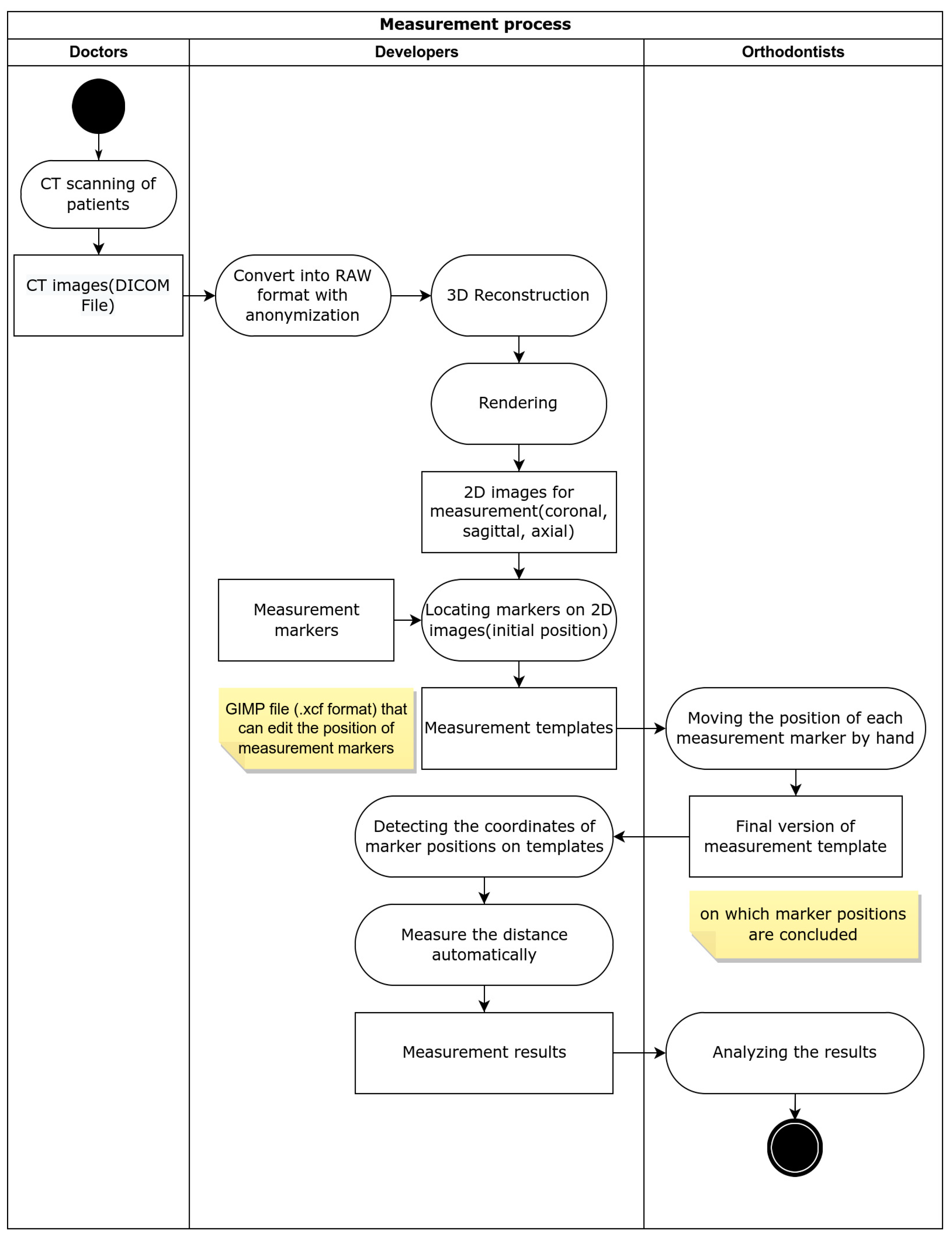
In Figure 1, an overview of the project in which this system is used is presented. The authors are referred to as Developers, the individuals responsible for placing markers are referred to as Orthodontists, and the providers of imaging data are referred to as Doctors.
2.2. Policy for Using Imaging Data
We received the computed tomographic (CT) images of 500 patients as digital imaging and communications in medicine (DICOM) files. Because the DICOM files included patients’ personal data, we removed the identifying information and anonymized the images by using RAW format. As a result, each patient is identified using only a four-digit serial number. The present study was approved by the Ethics Committee of Kanagawa Dental University (approval number: 841; date: 4 December 2021).
To simplify the automatic processing of these data, we created a batch script that converted DICOM files into RAW format when the files were received.
2.3. Creating Measurement Images
Measurement images are created using the process described in the next section. We adopted ExFact VR (Nihon Visual Science, Inc., Tokyo, Japan) for volume rendering.
First, we generated the anterior and lateral rendering images as orthogonal projections. These images are referred to in this article as “cephalograms”, although they are not cephalograms per se. We also generated axial slices of images of the nasal cavity.
Second, we set appropriate gradations of color and transparency on the screen to depict the intensity of each three-dimensional image by adjusting the look-up table (LUT) so that the viewer could easily recognize the landmarks in the rendered image.
This configuration affects the ease of recognition of the colors in each image and the clarity and inner contour of the image itself.
2.4. Automated Image Generation
Despite the need to create cephalograms for 500 people, the software used to render the volume data did not incorporate the ability to automatically generate cephalograms. Therefore, the aforementioned activity was handled by a script with process automation technology called “robotic process automation” (RPA); this enables automation that meets special needs arising at the field level without modifying the existing software. To accomplish this, we created a Python script to automatically control the software for volume rendering using PyAutoGUI, a module for graphical user interface (GUI) automation.
Additionally, we developed software that automatically calculates, generates, and applies the optimum LUT from the histogram of the intensity of the voxels of the input images and incorporates it into the script. The automatic generation of LUT may fail, depending on the distribution of the histogram. Therefore, we also made it possible to apply the LUT created in advance to the samples that the cephalograms failed to generate correctly.
2.5. Measurement Template
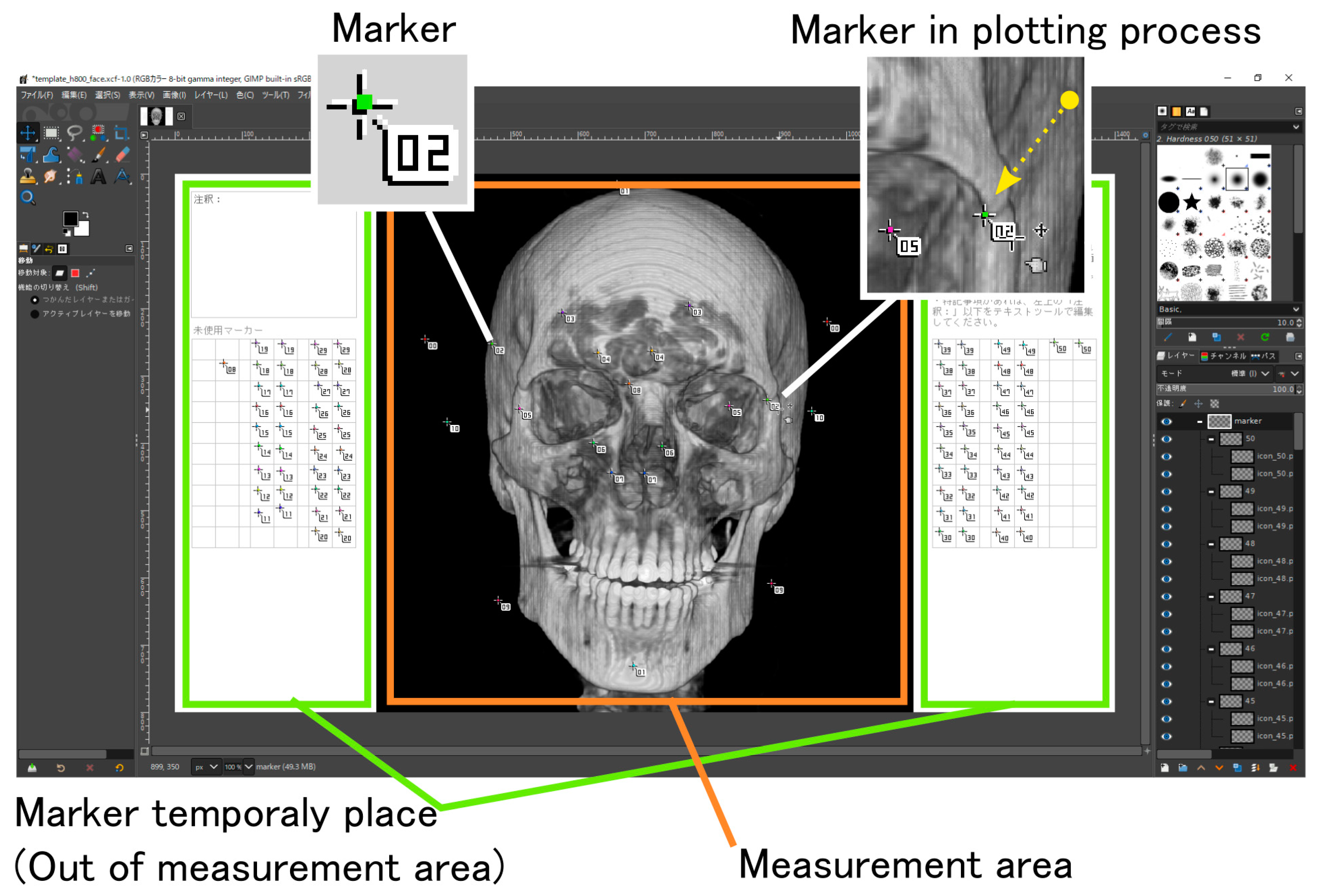
The measurement template (Figure 2) is an editable data image (in .xcf, a file format of GIMP) with some movable markers placed on the cephalogram to indicate the position of its landmarks. The markers’ positions are initially tentative. Developers devised template files in which orthodontists could indicate the landmarks.
The developers insert the cephalogram into the template where the marker is temporarily placed. Then, the developers send the template to orthodontists. The orthodontists move the markers to specified landmarks in the cephalograms and return the file to the developer.
The central part of the template (the area indicated by the orange frame as the measurement area in Figure 2) is the target of the measurement program’s processing. The markers placed in the storage areas (green frames in Figure 2) are ignored during measurement. In some of the imaging data we received, the scan range excluded some parts of the cranium; in some cases, the cranium was out of focus. In these cases, unnecessary markers could be moved to outside the measurement area to skip the measurement process.
Conversely, the measurement process with cephalograms must be repeated several times, with intervals between measurements, to minimize errors. The use of measurement templates does not require the repetition of the entire process to minimize errors. The measurement template with the correctable markers remains editable data. Therefore, if any measurement result is questionable, the measurement can be performed again after adjusting the positions of the markers that need to be corrected on the measurement template.
2.6. Marker Design
During the measurement process, the template is loaded into a program that automatically detects the position of the markers placed by the orthodontists. Each marker has a unique color, and the measurement program searches for pixels of that color to detect their position. The measurement marker is composed of the following elements (Figure 2):
- A balloon with a number;
- A point with a unique color that appears at the top of the balloon.
The marker is designed in anticipation of the manual work by the orthodontists and the processing by the position-detection program. The balloon not only indicates the marker ID but also helps the orthodontists grab and move it with the cursor.
2.7. Work Process via Measurement Template
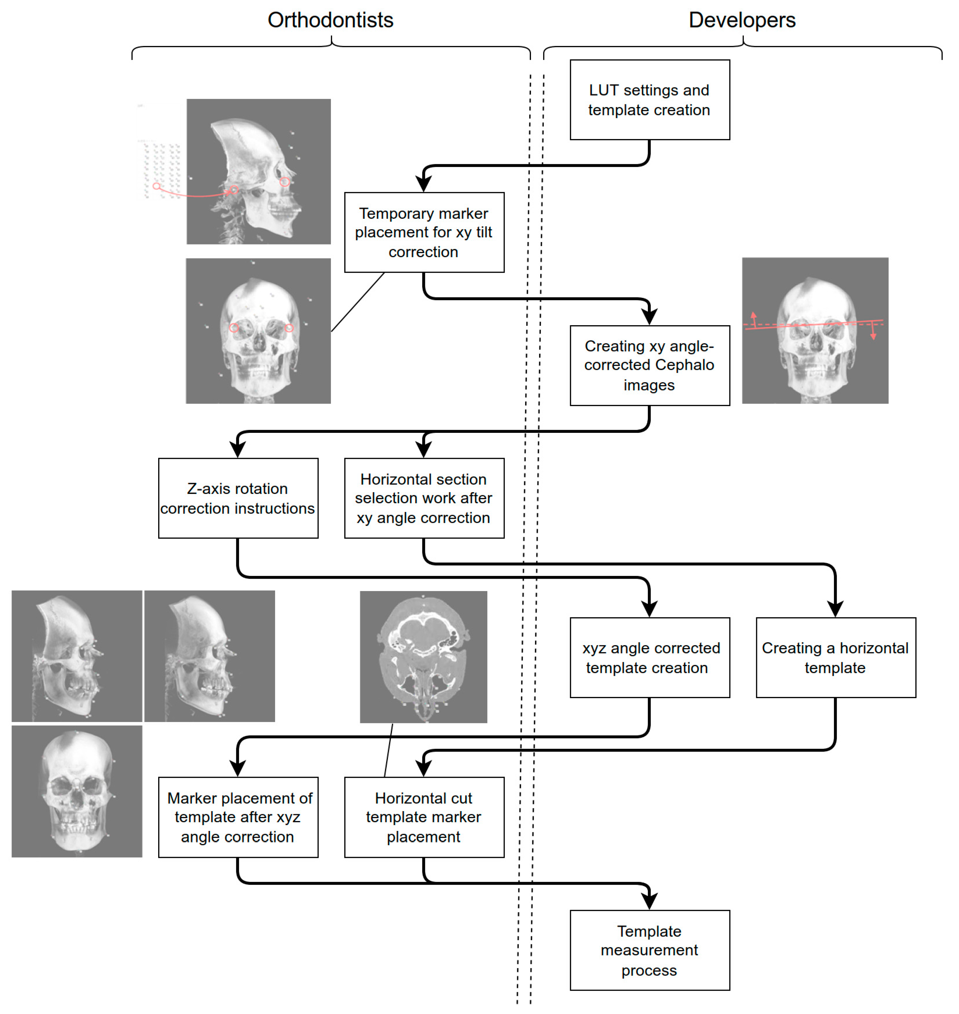
The measurement template is passed between the orthodontists and the developers, as shown in the top-to-bottom flow graphic in Figure 3. As indicated in the flow graphic, some aspects of the work might proceed simultaneously.
2.8. Tilt Correction
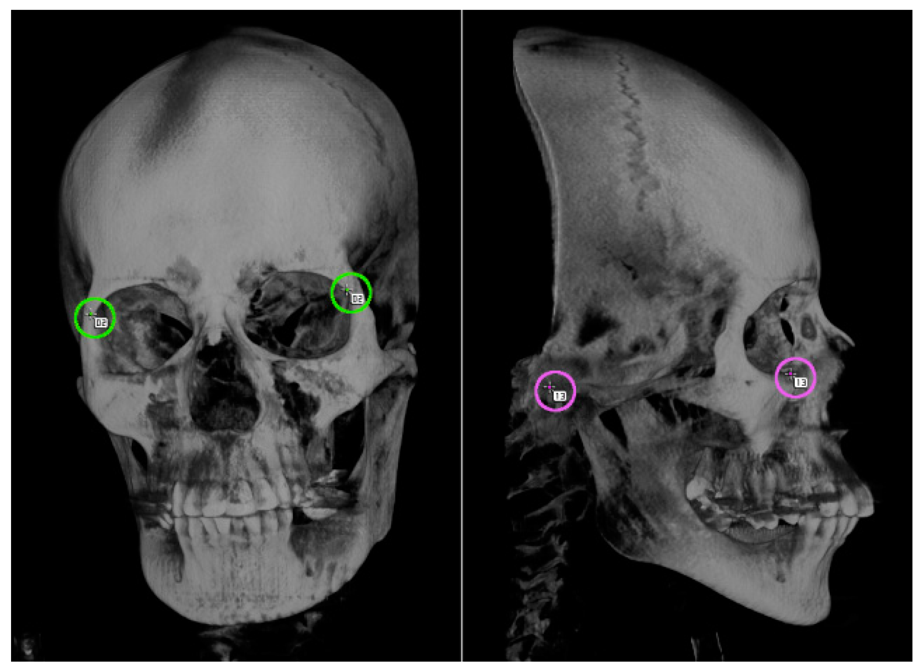
The craniofacial imaging data provided by doctors were not all straightforward. If the posture was inclined, the distances between the landmarks on the images would be compressed in the depth direction, which might result in inaccurate measurements. To prevent such compression, it was necessary to define the four landmarks for fixing the horizontal standard, to measure the two tilts of the axis, and to correct the inclinations of the imaging data before the actual measurements (Figure 4).
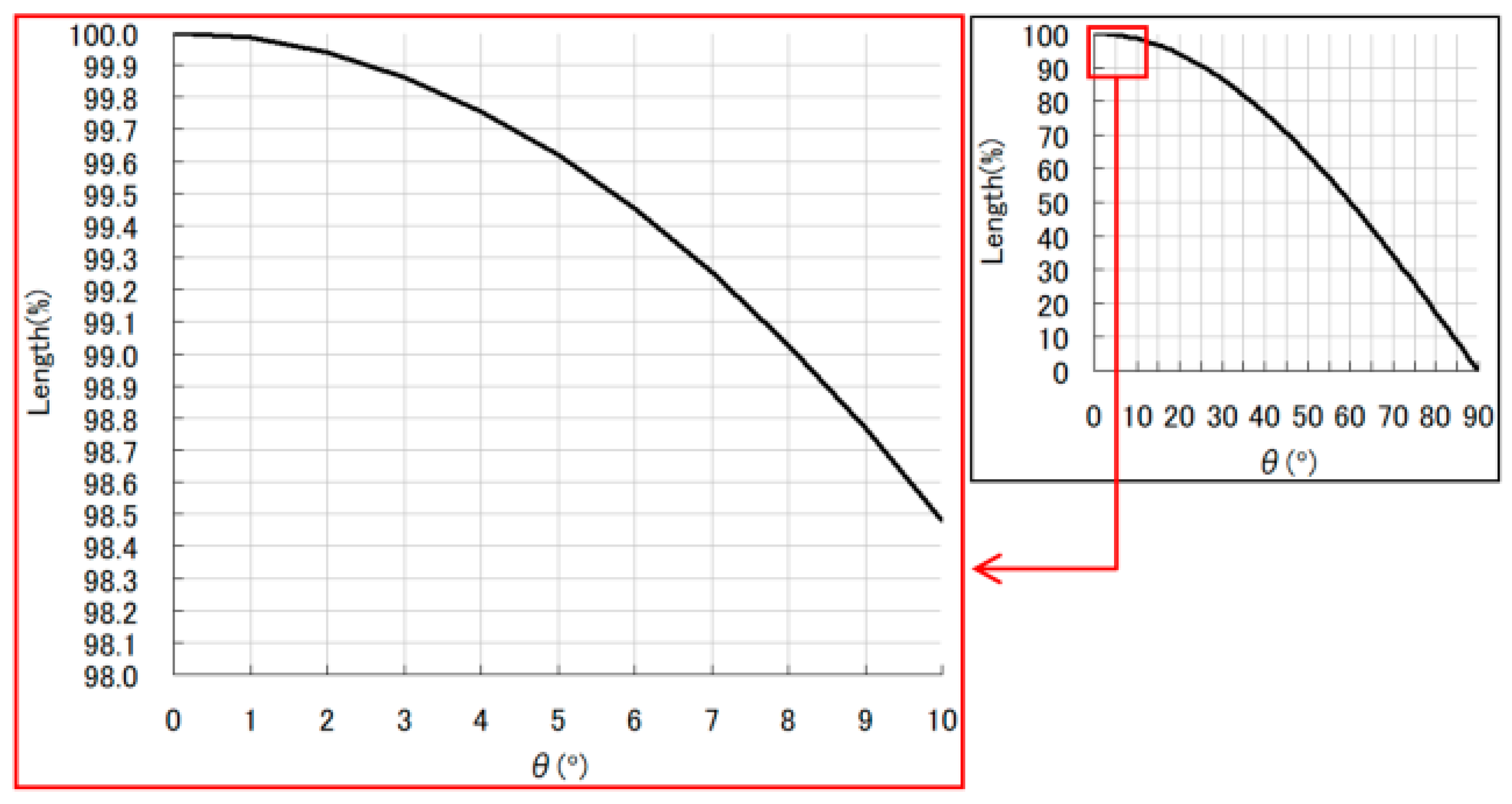
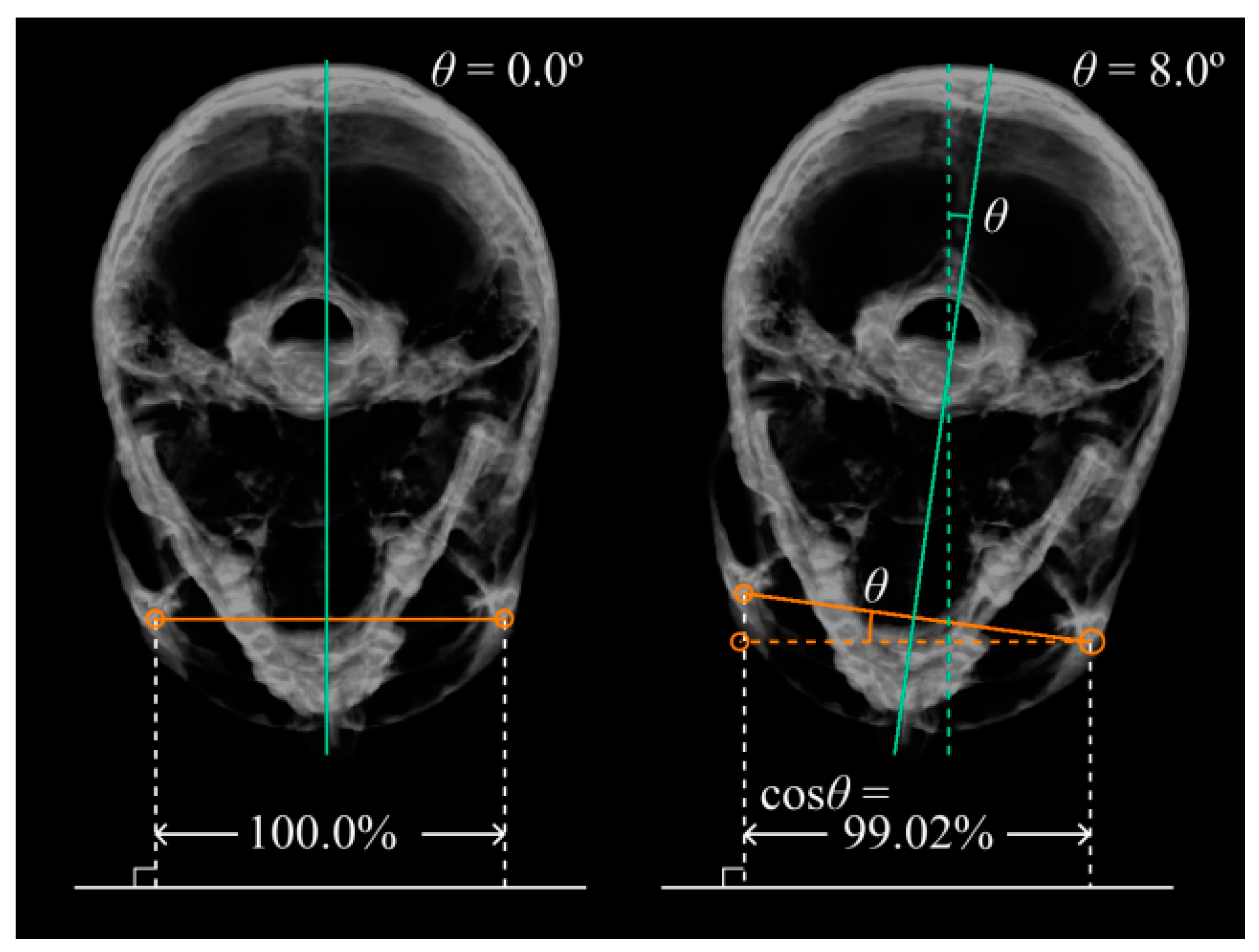
For example, it is assumed that the facial tilt of patients is characterized by front- and exact-side orientations of 0° and 90°, respectively. It is also assumed that the line connecting the left and right outermost edges of the orbits is horizontal and that its length is at its maximum when the patient is facing the front and at its minimum when the patient is facing exactly to the left side (Figure 5). If, instead, the patient is facing 8° to the left or right from the front, the measurement would be approximately 99.02% of the actual length (Figure 5 and Figure 6). In this case, if the actual length is 100 mm, the measurement would be 1 mm shorter. The error in the measurement increases rapidly as the inclinations increase.
The inclination of the horizontal tilt of the cranium was calculated from the positions of these four landmarks. By calculating back from that inclination, the inclination of roll and pitch rotation was corrected, and the horizontal orientations of the screen space and the cranium were matched. Regarding the yaw rotation, only the points that were inconsistent with the appearance of the rendered image were corrected. In this way, it was possible to easily identify the landmarks and obtain measurement images in which all the patients were shown in the ideal posture for measurement.
2.9. Operational Requirements
The following two points can be considered the error factors in the measurements:
- Resolution: the misalignment of the pixel scale;
- Accuracy: dispersion when the operator puts measurement markers on the images.
The first point refers to the limitation of resolution that results because the cephalogram in this system reflects not analog data, as a radiograph does, but sampled digital data. A digital image is constructed by pixels, and the position where a marker is placed can be determined only in units of pixels; a finer position adjustment is not possible. That is, the size of the pixels becomes the limit of the measurement resolution as it is.
In practice, the dispersion easily becomes an error factor rather than a limitation of the data. This is because, for some situations, the same landmark may be interpreted differently in centimeters by different orthodontists in placing the markers. Because marker placement criteria differ according to orthodontists, it was necessary to arrange the data in agreement with the images before the real measurement.
We distributed several examples of the same data to three orthodontists and asked them to arrange the markers; then, we overlapped their arrangements and checked the variations in position (Figure 8).
The orthodontists conferred with each other, referring to the images of the superimposed markers, confirming the difference in recognition of the correct marker position and discussing unified placement criteria. On the basis of the discussion, they made arrangements to practice marker placement together before proceeding to the actual work.
2.10. Definition of Landmarks to Be Measured
The following describes the actual required cephalometric specifications, as well as the measurement points and sections. These were based on the orthodontists’ research interests. Measurement images were conducted for five types, including front, left and right side views, and two types of cross sections. Depth distance was not considered, because distance measurement is performed on 2D images. Additionally, no angular measurements were taken, although it is technically possible to do so. The orthodontists and developers exchanged templates and decided on the landmarks that would be used in practice.
We present here an example of a measurement. Note that the measurement specifications follow the actual project, but the sample itself is data just for illustrative purposes.
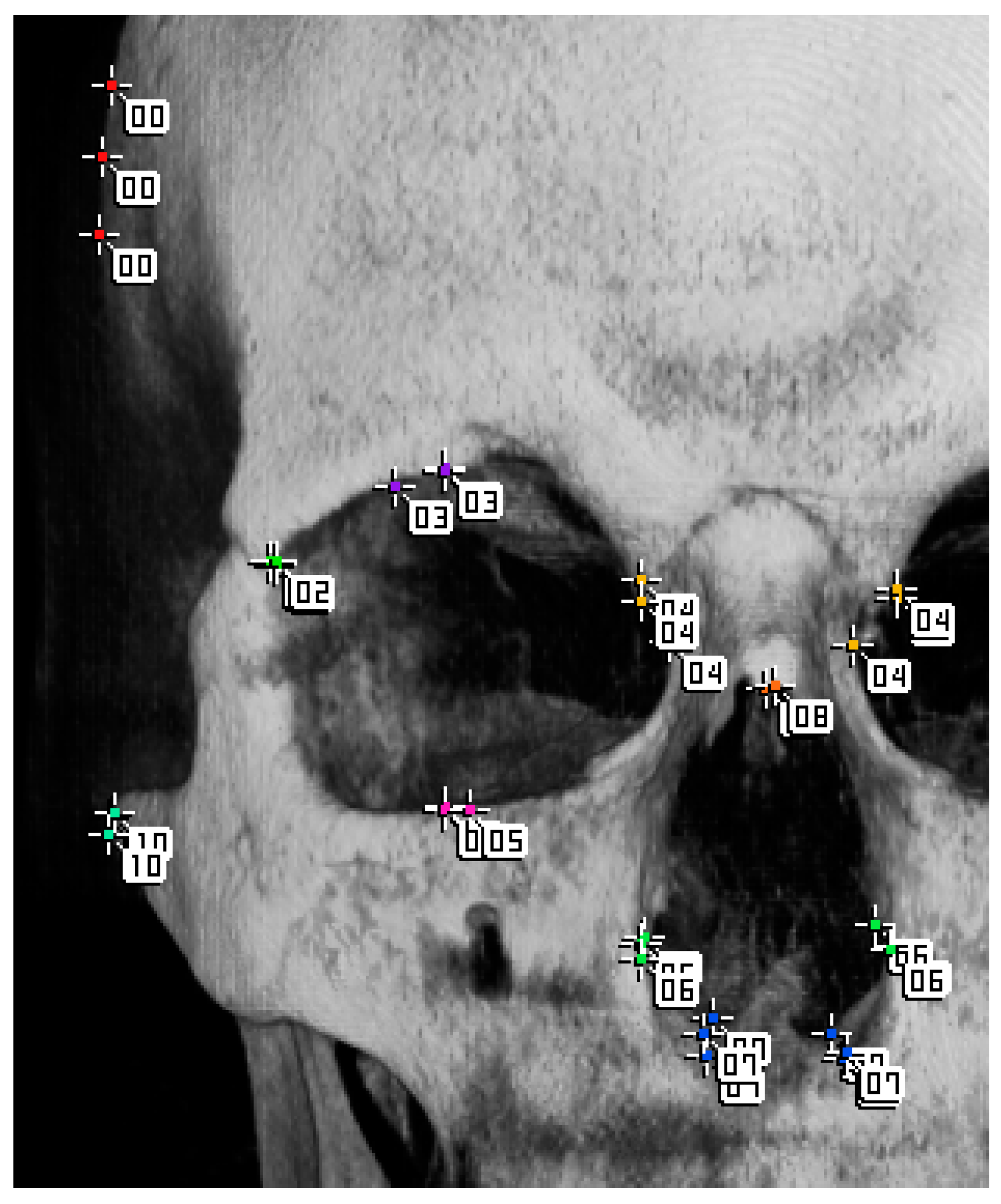
In the anterior template, 11 types of color-coded markers (21 markers in total) were used for the measurement (Figure 9).
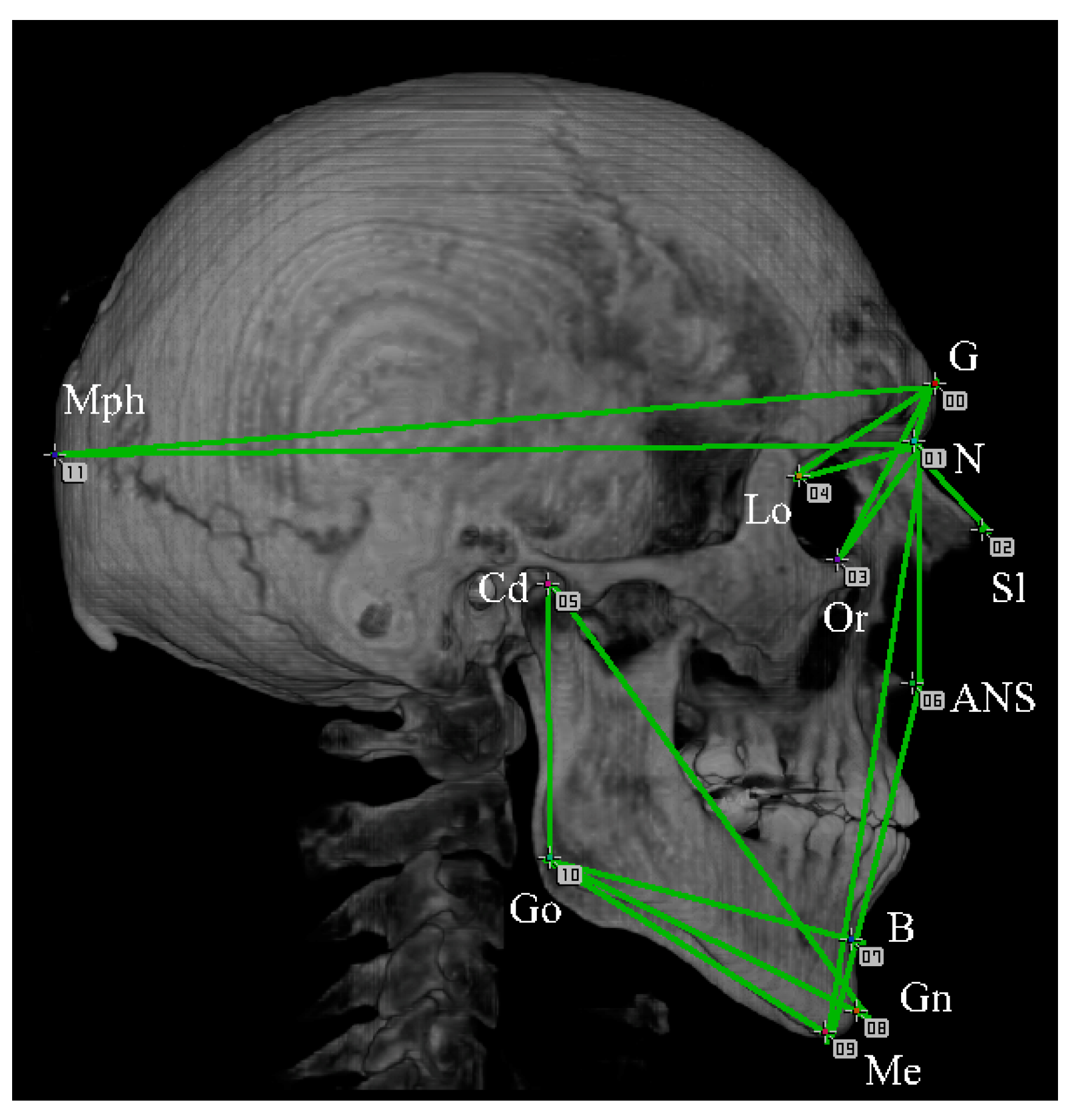
In the lateral template, 12 types of markers (12 markers in total) were used for the measurement (Figure 10). On each lateral measurement, two patterns of templates were created: one viewed from the left side of a cranium and the other viewed from the right side.
In axial templates, the pair of parallel cross-sectional slices was used (Figure 11).
2.11. Measurement Process
In the measurement process, the following three programs were used in order:
- template_to_image.py
- An image conversion script is a script that converts the marker placement template file of the original GIMP format into a portable network graphic (png) image file;
- This script is for the GIMP built-in Python shell, the same one used when the templates were created.
- point_detect.cpp
- Landmark detection program is a program that identifies the markers placed on the measurement image and outputs the coordinate values of each marker to a comma-separated values (csv) file;
- It is an easy C++ program in which image recognition is used.
- measure_distances.py
- A measurement script is a script that measures the required distance between each feature point from the combination of the coordinate values of each marker and the markers identified in the specifications;
- This script is a short Python script that calculates the distance from a csv file of coordinate values;
- The output results are several csv files of the distance between the markers.
3. Results
3.1. Format and Utilization of Aggregated Results
Figure 12 depicts the format of the csv file that shows the measurement results of the distance between the markers. The format detail is described as follows:
Row meaning:
- One row per patient.
Column meaning:
- First column: patient number;
- Second column: millimeter scale per pixel of the cephalogram (for reference);
- Third and subsequent columns: measurement results.
In a comparison of the values in the same column, the differences between the patients are easily shown through this format.
3.2. Example of Measurement
3.3. Operation
- Development and improvement were handled by four engineers;
- Data processing after routine use of the measurement process could be handled by one engineer;
- Three orthodontists participated, and we saw no need to increase the number.
3.4. Workload
For 500 patients:
- Five measurement images per patient (one front view, two side views, and two slices). A total of 2500 measurement images were prepared;
- For each patient, 49 measurement markers (21 for anterior, 24 for lateral, and 4 for slices) were expected to be placed;
- A total of 24,500 measurement marker placements (49 for each of 500 patients) were predicted;
- The actual number of markers placed was less than expected due to dispersions in imaging coverage;
- This workload was shared by three orthodontists;
- Each orthodontist was responsible for 100–200 patients;
- Length measurement was performed from the measurement template at 62 locations.
3.5. Evaluation
Speed:
- Throughput: when the project was live, data were exchanged approximately every 3 days to every week;
- Latency time: data aggregation time was several minutes for all 500 patients.
Period:
- This project progressed to the final stage, and it was developed and improved over the course of a little over a year.
Accuracy:
- Accuracy is guaranteed using measurements made after the markers were placed by orthodontists who had anatomical knowledge.
4. Discussion
4.1. Verification of Results
The evaluation of the results presented in this study should be discussed in terms of the validity of the measurement results and the efficiency of the measurement process. As stated in the Results section, the validity of the measurement results obtained using this system was acknowledged by the measurement requesters themselves, who possess expertise in the relevant field. By contrast, in respect of the evaluation of the efficiency of this method, as we could find only a small number of papers describing the time required for these measurements [10], we discussed the relationship between estimated and spent time in the actual measurement project. In the preparation stage of the measurement project that was addressed in this study, a discussion on the efficiency of comparison with existing methods had already been conducted. Specifically, from the perspective of practitioners and scholars in the field of orthodontics, the introduction of a new system in the measurement project was required for the completion of a large number of measurements in a short period, and the deadline was set accordingly. As a result, the measurement project using this system successfully delivered all the measurement results within the deadline. Based on the fact that the above goals have been achieved, the efficiency of this system can be considered to have been proven.
4.2. Significance of the System
The proposed system, as shown in the flowchart in Figure 1, allows for the simplification and automation of individual processes, allowing for a collaborative and streamlined workflow among workers with the appropriate skills. This leads to improved efficiency and accurate results. Moreover, the strength of the system lies in its ability to allow for a seamless workflow even when the workers are temporally or spatially separated, as long as data transfer is successful. In this case, it is also possible to implement an asynchronous operation in which the results are accumulated for each task and the measurement process is performed after a certain amount of data are collected. This allows for the appropriate allocation of personnel and equipment according to the workload of each process.
Thus, the system and method of operation adopted in this study enable overall efficiency and flexible operation in the processing.
4.3. Limits
This system is supposed to be able to measure angles, areas, etc.; however, in THE actual measurement implemented in our project, only simple length measurements have been performed.
This system has limitations in measurement resolution due to the use of digital images. Additionally, in the division of labor, there is a bias that arises from the fact that people perform measurements visually. This was eliminated by forming a consensus among the workers. In the consensus-building discussions, the measurement template was effective in clearly demonstrating bias.
4.4. Future Outlook
Looking ahead, during the building and operation of inspection systems for industries, food production, and the medical field, there may be cases where it is not possible to eliminate human judgment. Even if the automation of processing using AI is envisaged, the system cannot reach a state of completion all at once.
By adopting measurement templates and operating methods like this, it is possible to accumulate not only the results of measurements but also the data from the operating inspection and the diagnostic system’s processes that rely on visual judgment. Owing to this, it is possible to expect educational benefits as beginners learn to apply the method of image judgment using the marker positions set by experienced workers. Furthermore, these data can also be used as training data for AI-based recognition, and by improving its accuracy, it will be possible to transition to complete automation gradually and without difficulty.
5. Conclusions
Employing a system that combines manual work with automation using measurement templates and dental and maxillofacial measurement, a small number of orthodontists were able to proceed without delay using the CT-imaging data of 500 patients, and accurate results were obtained.
Author Contributions
Conceptualization, K.T.; Methodology, K.T.; Software, K.T.; Validation, A.M.; Investigation, A.M.; Writing—Original Draft Preparation, H.K.; Project Administration, H.K.; Funding Acquisition, K.T. All authors have read and agreed to the published version of the manuscript.
Funding
Harumichi KOGA (corresponding author) is paid by Nihon Visual Science, Inc., Tokyo, Japan(NVS), https://www.nvs.co.jp/ (accessed on 9 March 2023). NVS was paid by Tetsutaro YAMAGUCHI of Kanagawa Dental University, Japan (KDU) for the development of the system covered in the manuscript, https://researchmap.jp/read0058115 (accessed on 9 March 2023). Tetsutaro YAMAGUCHI funded the development of this system with research funding from Grants-in-Aid for Scientific Research (KAKENHI) from the Ministry of Education, Culture, Sports, Science, and Technology, Japan, https://nrid.nii.ac.jp/ja/nrid/1000040384193/ (accessed on 9 March 2023).
Institutional Review Board Statement
Not applicable.
Informed Consent Statement
Not applicable.
Data Availability Statement
The data can be obtained by contacting [email protected].
Acknowledgments
The authors would like to thank Miwa Isogai, a senior student in the Division of English, Tokyo Women’s Christian University, for her help in the translation of this paper and several research studies related to its submission. The authors would like to thank Enago (www.enago.jp) (accessed on 9 March 2023) for the English language review.
Conflicts of Interest
NVS plan to patent the content of the treatise and make a profit from it.
References
- Broadbent, B.H. A new X-ray technique and its application to orthodontia. Angle Orthod. 1931, 1, 45–66. [Google Scholar]
- Adel, M.; Yamaguchi, T.; Tomita, D.; Nakawaki, T.; Kim, Y.I.; Hikita, Y.; Haga, S.; Takahashi, M.; Nadim, M.A.; Kawaguchi, A.; et al. Contribution of FGFR1 variants to craniofacial variations in East Asians. PLoS ONE 2017, 12, e0170645. [Google Scholar] [CrossRef] [PubMed]
- Yamaguchi, T.; Maki, K.; Shibasaki, Y. Growth hormone receptor gene variant and mandibular height in the normal Japanese population. Am. J. Orthod. Dentofac. Orthop. 2001, 119, 650–653. [Google Scholar] [CrossRef] [PubMed]
- Gribel, B.F.; Gribel, M.N.; Frazão, D.C.; McNamara, J.A., Jr.; Manzi, F.R. Accuracy and reliability of craniometric measurements on lateral cephalometry and 3D measurements on CBCT scans. Angle Orthod. 2011, 81, 26–35. [Google Scholar] [CrossRef] [PubMed]
- Bajaj, K.; Rathee, P.; Jain, P.; Panwar, V.R. Comparison of the reliability of anatomic landmarks based on PA cephalometric radiographs and 3D CT scans in patients with facial asymmetry. Int. J. Clin. Pediatr. Dent. 2011, 4, 213–223. [Google Scholar] [PubMed]
- Kim, H.; Shim, E.; Park, J.; Kim, Y.J.; Lee, U.; Kim, Y. Web-based fully automated cephalometric analysis by deep learning. Comput. Methods Programs Biomed. 2020, 194, 105513. [Google Scholar] [CrossRef] [PubMed]
- Hung, K.; Montalvao, C.; Tanaka, R.; Kawai, T.; Bornstein, M.M. The use and performance of artificial intelligence applications in dental and maxillofacial radiology: A systematic review. Dento. Maxillo. Fac. Radiol. 2020, 49, 20190107. [Google Scholar] [CrossRef] [PubMed]
- Urooge, A.; Patil, B.A. Sexual dimorphism of maxillary sinus: A morphometric analysis using cone beam computed tomography. J. Clin. Diagn. Res. 2017, 11, ZC67–ZC70. [Google Scholar] [CrossRef] [PubMed]
- Alhazmi, A. Association between maxillary sinus dimensions and midface width: 2-D and 3-D volumetric cone-beam computed tomography cross-sectional study. J. Contemp. Dent. Pract. 2020, 21, 317–321. [Google Scholar] [CrossRef] [PubMed]
- Mosleh, M.A.A.; Baba, M.S.; Malek, S.; Almaktari, R.A. Ceph-X: Development and evaluation of 2D cephalometric system. BMC Bioinform. 2016, 17, 499. [Google Scholar] [CrossRef] [PubMed]
Figure 1.
An overview of the project in which this system is used. The .xcf file is a file format handled by the freeware GIMP: GNU image manipulation program. CT: computerized tomography; DICOM: digital imaging and communication in medicine; 3D: three-dimensional; 2D: two-dimensional.
Figure 1.
An overview of the project in which this system is used. The .xcf file is a file format handled by the freeware GIMP: GNU image manipulation program. CT: computerized tomography; DICOM: digital imaging and communication in medicine; 3D: three-dimensional; 2D: two-dimensional.

Figure 2.
Measurement template opened in GIMP. Since the markers are divided into individual layers, its position can be adjusted individually.
Figure 2.
Measurement template opened in GIMP. Since the markers are divided into individual layers, its position can be adjusted individually.

Figure 3.
Details of the workflow using measurement templates. The dotted line separates the right and left sides, which represent the work of the developers and orthodontists, respectively.
Figure 3.
Details of the workflow using measurement templates. The dotted line separates the right and left sides, which represent the work of the developers and orthodontists, respectively.

Figure 4.
Four points used as a horizontal reference on the skeleton. Anterior image (left) and lateral image (right). To calculate the tilt of the skeleton with respect to the horizontal plane, images viewed from at least two directions are required.
Figure 4.
Four points used as a horizontal reference on the skeleton. Anterior image (left) and lateral image (right). To calculate the tilt of the skeleton with respect to the horizontal plane, images viewed from at least two directions are required.

Figure 5.
Change in the length of a horizontal line defined on the face on the screen in response to changes in the (left and right) orientation of the face. The graphs on the right and left show the ranges of 0°–90° and 0°–10°, respectively.
Figure 5.
Change in the length of a horizontal line defined on the face on the screen in response to changes in the (left and right) orientation of the face. The graphs on the right and left show the ranges of 0°–90° and 0°–10°, respectively.

Figure 6.
Figure 4 shown using the image of the section of the patient. The image is seen from the top. The line at the bottom of the figure represents the screen plane. The left side of the figure is facing the front, and the right side is 8° facing left to the screen plane. For the correction of anterior tilt, as in the top left image of Figure 7, the line connecting the two intersections of the orbit and each orbital line is defined as the horizontal standard. For the correction of lateral tilt, as in the top right image of Figure 7, the line connecting the lowest point of the orbit and the uppermost point of the upper edge of the ear canal was defined as the horizontal standard. The setting of these reference points and the placement of the markers on the reference points are performed by the orthodontist.

Figure 7.
Progress of tilt correction. The left column is an anterior image, and the right column is a lateral image. The upper row is the correction of the inclination with respect to the horizontal plane. The points represent the landmarks used for correction, the broken lines are the reference plane, and the solid lines are the slopes with respect to the reference plane. The result of the tilt correction is shown by the solid line in the middle row. The middle row corrects the deviation in the front direction. The dashed line represents the axis of rotation. The lower row shows the state where all tilt corrections have been completed.

Figure 8.
Measurement markers individually placed by three orthodontists for the same patient are superimposed on one image. Three markers with the same number are placed, and each position is misaligned. There is little deviation in the placement of marker 02. In contrast, marker 00 is placed differently by each orthodontist.

Figure 9.
Markers and measurement intervals used in anterior images. The measurement intervals are 28 sections indicated by connecting the measurement points with lines. 00: (Eu) eunion, 01(upper): (Th) top of head, 01(lower): (Me) menton, 02: (Lo) the oblique orbital line, 03: (Ro) root of orbit, 04: (Io) inside of orbit, 05: (Bo) bottom of orbit, 06: (Al) allare, 07: (Sub) subnasale, 08: (Sel) sellion, 09: (Go) gonial, and 10: (Zyg) zygoma.

Figure 10.
Markers and measurement intervals used in anterior images. The measurement intervals are 16 sections indicated by connecting the measurement points with lines. 00: (G) glabella, 01: (N) nasion, 02: (Sl) sellion, 03: (Or) orbitale, 04: (Lo) the oblique orbital line, 05: (Cd) condyle, 06: (ANS) anterior nasal spine, 07: (B) point B, 08: (Gn) gnasion, 09: (Me) menton, 10: (Go) gonion, and 11: (Mph) the most posterior point of head.

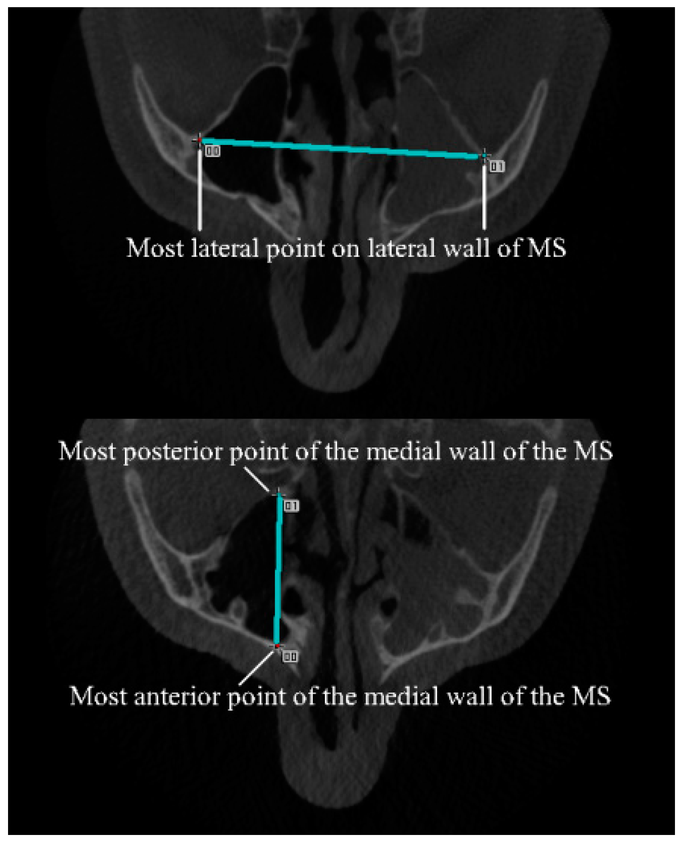
Figure 11.
Markers and measurement intervals used in axial slice images. For each slice of section, two types of markers are used: one marker for each, for a total of two markers, and four on slice measurement. (MS) maxillary sinus. Top: section to measure maxillary sinus width [8]. Bottom: section to measure nasal length [9].

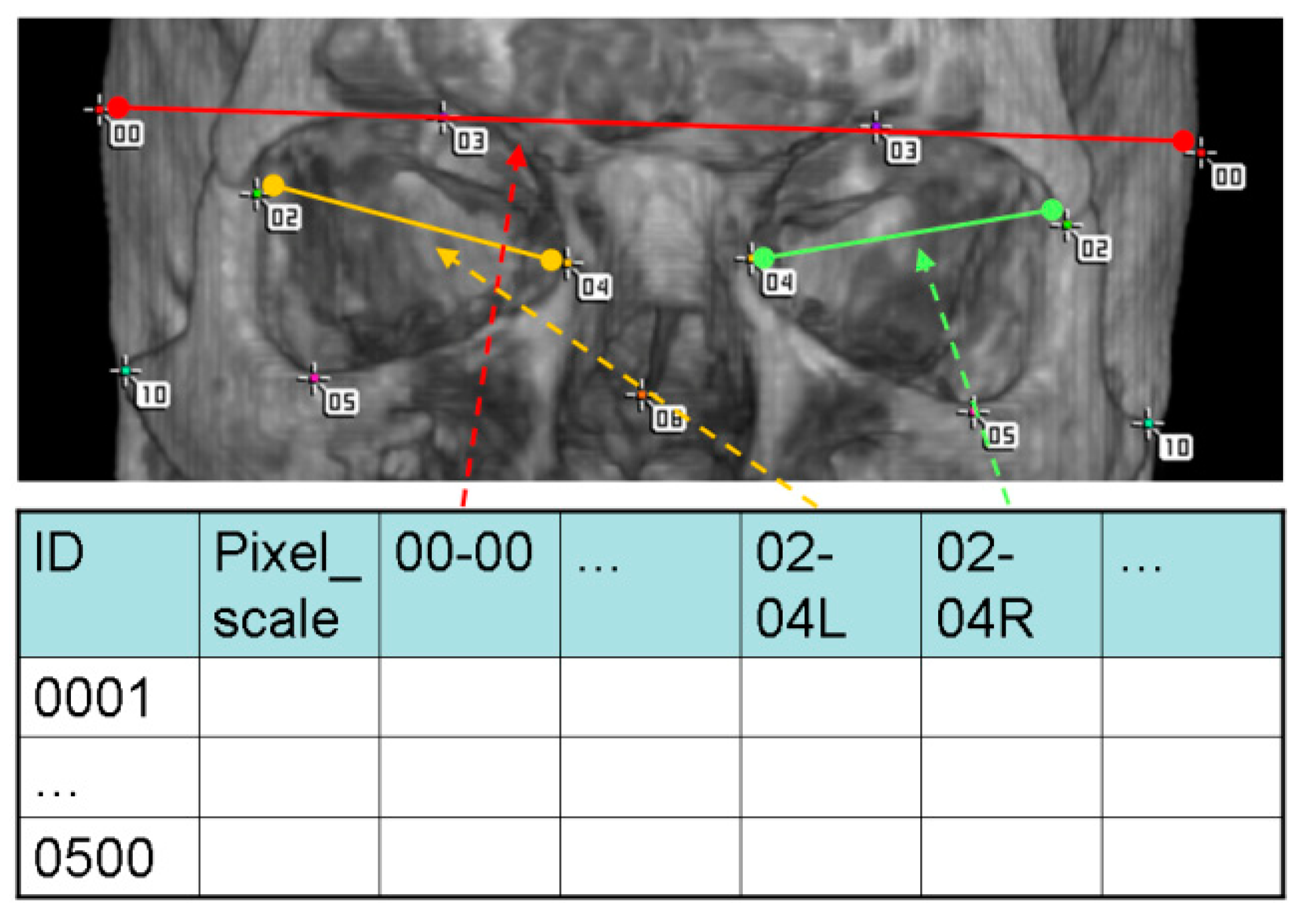
Figure 12.
An example of the csv file format of the result and the corresponding section on the measurement image. In the actual file, the value of the length in mm is entered in each cell as the measurement result. The column name represents the measurement interval and is in the format of “aa--bbL/R.” “aa” is the marker number of the start point; “bb” is the marker number of the end point. If the left and right measurements differ, “L”/“R” will be attached. Each value of the cell (in millimeters) is the distance from the start point to the end point.


Table 1.
Results of anterior measurements.
| Distance (mm) | |||
|---|---|---|---|
| Section | Center | Left | Right |
| 00--00 | 151.92 | - | - |
| 01--01 | 232.57 | - | - |
| 02--02 | 110.72 | - | - |
| 02--03 | - | 20.96 | 22.61 |
| 02--04 | - | 44.99 | 42.35 |
| 02--05 | - | 26.47 | 28.56 |
| 03--03 | 72.59 | - | - |
| 03--04 | - | 32.3 | 28.03 |
| 03--05 | - | 36.71 | 36.91 |
| 04--04 | 24.81 | - | - |
| 04--05 | - | 39 | 34.48 |
| 05--05 | 89.36 | - | - |
| 06--06 | 29.53 | - | - |
| 06--07 | - | 14.01 | 12.55 |
| 06--08 | - | 28.72 | 28.84 |
| 07--07 | 16.74 | - | - |
| 07--08 | - | 37.77 | 36.8 |
| 09--09 | 108.95 | - | - |
| 10--10 | 138.02 | - | - |
Table 2.
Results of lateral measurements.
| Distance (mm) | ||
|---|---|---|
| Section | Left | Right |
| 00--01 | 14.42 | 12.82 |
| 00--03 | 53.03 | 47.21 |
| 00--04 | 39.9 | 36.51 |
| 00--11 | 214.55 | 214.19 |
| 01--02 | 26.2 | 24.89 |
| 01--03 | 38.65 | 34.42 |
| 01--04 | 28.63 | 26.92 |
| 01--06 | 57.97 | 58 |
| 01--09 | 144.38 | 145.73 |
| 01--11 | 207.73 | 207.08 |
| 05--08 | 123.8 | 129.83 |
| 05--10 | 68.54 | 68.03 |
| 06--09 | 87.6 | 89.26 |
| 07--10 | 77.21 | 75.89 |
| 08--10 | 81.28 | 81.66 |
| 09--10 | 75.71 | 78.25 |
Table 3.
Results of axial measurements.
| Distance (mm) | ||
|---|---|---|
| Section | Maxillary Sinus Width | Nasal Length |
| 00--01 | 84.66 | 41.87 |
Disclaimer/Publisher’s Note: The statements, opinions and data contained in all publications are solely those of the individual author(s) and contributor(s) and not of MDPI and/or the editor(s). MDPI and/or the editor(s) disclaim responsibility for any injury to people or property resulting from any ideas, methods, instructions or products referred to in the content. |
© 2023 by the authors. Licensee MDPI, Basel, Switzerland. This article is an open access article distributed under the terms and conditions of the Creative Commons Attribution (CC BY) license (https://creativecommons.org/licenses/by/4.0/).
Share and Cite
MDPI and ACS Style
Koga, H.; Taki, K.; Masugi, A. Efficient Measurement Method: Development of a System Using Measurement Templates for an Orthodontic Measurement Project. Software 2023, 2, 276-291. https://doi.org/10.3390/software2020013
AMA Style
Koga H, Taki K, Masugi A. Efficient Measurement Method: Development of a System Using Measurement Templates for an Orthodontic Measurement Project. Software. 2023; 2(2):276-291. https://doi.org/10.3390/software2020013
Chicago/Turabian StyleKoga, Harumichi, Katsuhiko Taki, and Ayano Masugi. 2023. "Efficient Measurement Method: Development of a System Using Measurement Templates for an Orthodontic Measurement Project" Software 2, no. 2: 276-291. https://doi.org/10.3390/software2020013