Article

Transforming a Computational Model from a Research Tool to a Software Product: A Case Study from Arc Welding Research

1
CSIRO Manufacturing, Lindfield, NSW 2070, Australia
2
CSIRO Data61, Clayton South, VIC 3169, Australia
3
CSIRO Manufacturing, Clayton South, VIC 3169, Australia
4
CSIRO Mineral Processing, Clayton South, VIC 3169, Australia
*
Author to whom correspondence should be addressed.
Software 2023, 2(2), 258-275; https://doi.org/10.3390/software2020012
Submission received: 3 March 2023 / Revised: 5 May 2023 / Accepted: 6 May 2023 / Published: 8 May 2023

Abstract

:
Arc welding is a thermal plasma process widely used to join metals. An arc welding model that couples fluid dynamic and electromagnetic equations was initially developed as a research tool. Subsequently, it was applied to improve and optimise industrial implementations of arc welding. The model includes the arc plasma, the electrode, and the workpiece in the computational domain. It incorporates several features to ensure numerical accuracy and reduce computation time and memory requirements. The arc welding code has been refactored into commercial-grade Windows software, ArcWeld, to address the needs of industrial customers. The methods used to develop ArcWeld and its extension to new arc welding regimes, which used the Workspace workflow platform, are presented. The transformation of the model to an integrated software application means that non-experts can now run the code after only elementary training. The user can easily visualise the results, improving the ability to analyse and generate insights into the arc welding process being modelled. These changes mean that scientific progress is accelerated, and that the software can be used in industry and assist welders’ training. The methods used are transferrable to many other research codes.

1. Introduction

Computational modelling is a core activity for research groups worldwide in academia, government institutions, and industry. Though commercial software packages are increasingly used, many groups continue to write and maintain their own computer codes, often because the commercial packages do not meet their needs. In most cases, the codes are developed as research tools and are configured for use by highly trained research scientists and engineers. Though this approach saves the significant effort required to develop user interfaces, automate procedures, and integrate visualisation of the results, it has several drawbacks. The usefulness of such codes to industry and other collaborators is limited since weeks of training are typically required to understand the intricacies of running the computer code. Further, such models generally cause difficulties with version control, input and output file management, and related matters.
Factors such as increasing interactions between academic researchers and industry and the growing emphasis on data retention are motivating the refactoring of research codes into user-friendly, maintainable software.
The primary purposes of this paper are to (1) outline the approach used to transform a computer code developed as a research tool into an easily accessible software package and (2) describe the good practices that have been applied and emphasise the benefits that have resulted from the changes. Though we focus on a specific example, a computational model of arc welding, both the general principles and the specific methods presented are broadly applicable to a vast range of computational models, since our approach is readily transferrable, and the benefits are universally applicable. Therefore, we expect the study to be of wide interest to those involved in or responsible for computational models.
We begin by providing some context for the specific example of arc welding and the motivation for the work. Arc welding is an example of a thermal plasma process. Many important industrial processes, including arc welding, wire-arc additive manufacturing, plasma cutting, and plasma spraying, are based on thermal plasmas. The plasma is usually produced by an electric arc between two electrodes, providing peak temperatures that exceed 10,000 K [1,2,3,4] (and in some cases, 20,000 K [5,6]) and intense heat fluxes. Thermal plasmas typically operate at or close to atmospheric pressure. They are fluids and can be modelled using computational fluid dynamics. For thermal plasmas in which the flow speed is well under the speed of sound, such as welding arcs, the appropriate equations are those for viscous incompressible flow, an energy conservation equation, and equations derived from Maxwell’s equations to treat the electromagnetic phenomena. Source terms are included to handle effects such as the Lorentz force, Joule heating, and radiative cooling [7,8,9].
Many researchers have developed plasma modelling codes, for example, for thermal plasma processes [9], including nanoparticle production [10,11,12], plasma jet formation [13], and waste destruction [14], as well as low-pressure plasma processes for applications such as semiconductor etching [15,16], deposition [16], and lighting [17].
There have been several significant advances with such models over the past 30 years. For example, in arc welding models:
  • Initially, only the arc plasma was modelled, with the influence of electrodes included using boundary conditions; now, the electrodes and other materials that interact with the plasma are included within the computational domain;
  • The models were initially one- or two-dimensional and steady-state but can now be three-dimensional and time-dependent;
  • Though the modelling effort was directed initially toward providing scientific insights to help understand experimental results, models are now being used to develop and improve industrial processes.
Such changes have significantly increased the relevance and attractiveness of plasma models to industrial users.
An example of a sophisticated thermal plasma model is CSIRO’s model of metal inert gas/metal active gas (MIG/MAG) welding, also known as gas metal arc welding (GMAW). MIG/MAG welding is the most widely used arc welding process in manufacturing industries. The extension and adaptation of the model to MIG/MAG welding were partly funded by a customer in the automotive industry, General Motors, with a focus on the welding of sheet aluminium. The customer requested that the computer code be packaged for use by its welding engineers and technicians. The code was refactored using the Workspace workflow platform [18,19,20] to fulfil this request, allowing the existing modelling code to be run under Windows on a standard desktop or notebook computer. A simple graphical user interface (GUI) was introduced for the entry of input parameters, running the computer code, displaying progress towards convergence, and providing graphical visualisation of the results. This was all achieved with a very low development cost. The resulting software package is called ArcWeld.
A subsequent customer requested the extension of the model to treat different metals, shielding gases and welding geometries. The flexibility of the Workspace platform allowed these changes to be rapidly incorporated into the GUI.
It is worth noting that commercial software packages for arc welding exist, for example, SYSWELD [21]. SYSWELD uses finite element analysis (FEA), which allows residual stresses and distortion to be predicted in complex welded structures. In such packages, however, the arc plasma is not modelled. Instead, the effect of the arc plasma on the workpiece is calculated using source terms for the heat flux and, in some cases, the pressure and the electric current density. Moreover, the flow in the weld pool is not modelled, so its influence has to be included in the heat flux source term. The CFD (computational fluid dynamics) software package FLOW-3D (version 7.7) [22] has been used for arc welding modelling [23]. Though FLOW-3D allowed the flow in the weld pool to be modelled, the arc plasma was represented by heat flux and arc pressure source terms on the weld pool surface. FLOW-3D also provides a welding module, FLOW-3D Weld [24], but this is configured for laser welding and cannot be applied to arc welding.
Different expressions for the distribution of the heat source and other quantities can be used [23,25,26,27]. They all have several free parameters (representing, for example, the arc efficiency and the physical dimensions of the source term), which are typically obtained by comparison of the predictions of the software with measurements of weld cross-sections and thermal history at positions in the workpiece. Such experiments are time-consuming and expensive. Since the free parameters depend on factors such as the arc current, welding speed, and electrode angle, the experiments must be repeated when these factors change significantly. In addition, the expressions cannot account for the two-way interactions between the arc and weld pool, such as the production of metal vapour, which affects the arc and weld properties.
Section 2 presents the methods used in developing the ArcWeld software package. In Section 2.1, we present a summary of the computational model of MIG/MAG welding that forms the basis of the ArcWeld software and note some of the good practices used in its development. The arc welding code that was developed is available as a file executable from the command line. A semi-manual workflow was used to run the code and record results. To refactor the code into commercial-grade software, an intuitive GUI was developed to provide an easy-to-use interface. Workspace [28] was used to create a wrapper around the command-line interface, preparing the required input files, calling the binary executable, and monitoring results from output files written to disk by the executable. We describe the code operation before this refactoring in Section 2.2 and outline the process by which the refactoring was performed, and the software subsequently extended, in Section 2.3.
We then describe, in Section 3, the results achieved, particularly the changes to the workflow introduced by packaging the code with a GUI using Workspace. Section 4 considers the benefits of such an approach to improving simulation practice and the translation of research to a useful product from both researcher and industrial collaborator perspectives.

2. Materials and Methods

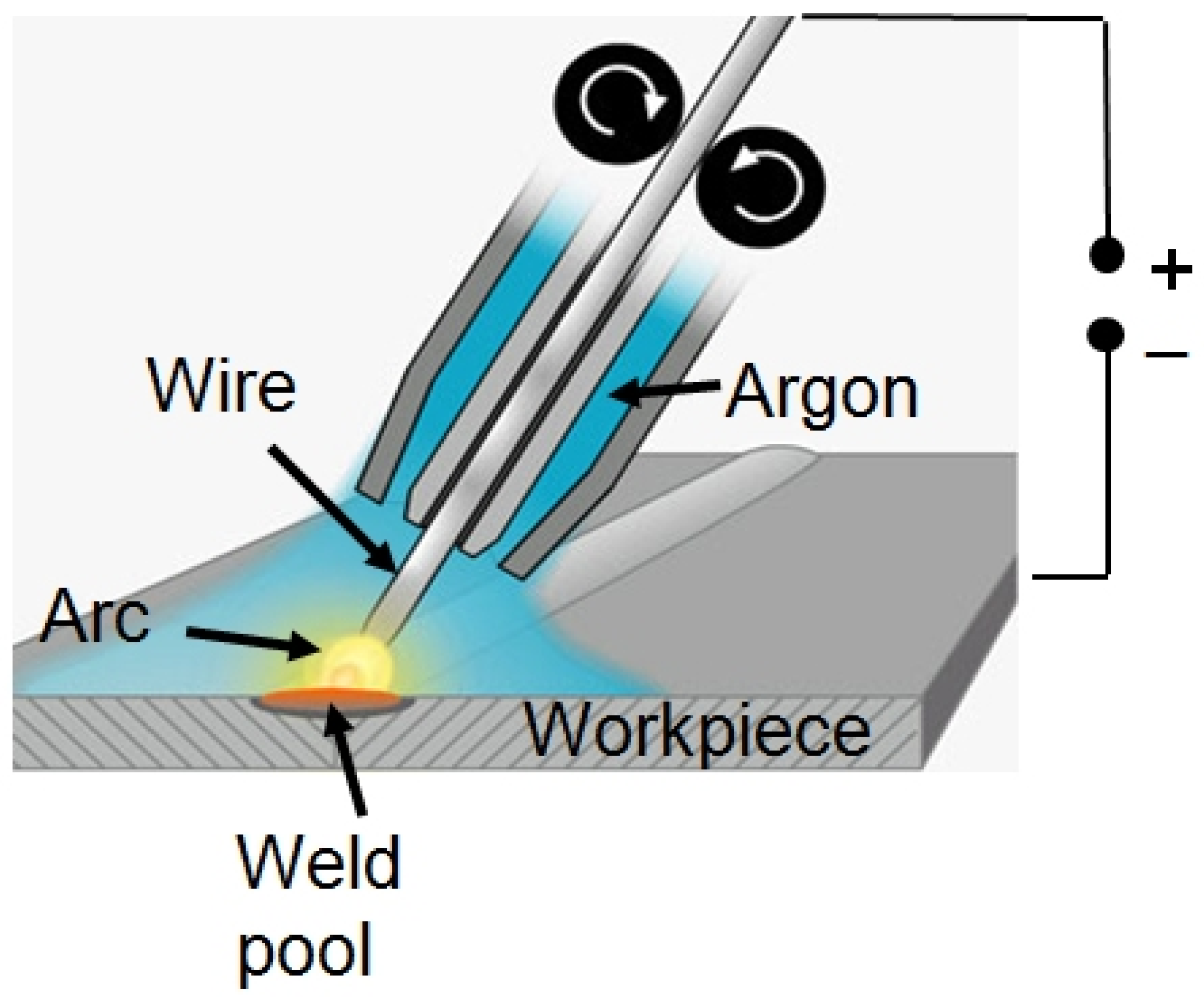
2.1. The Computational Model of MIG/MAG Welding

MIG/MAG welding uses the intense heat flux produced by an arc plasma to partially melt two pieces of metal, which are joined when the molten region (the weld pool) solidifies. The arc plasma is formed in the shielding gas between the two electrodes. One electrode, typically the anode, is a metal wire. The other, known as the workpiece or the base metal, is the pieces of metal being joined. The wire melts, producing droplets of liquid metal that pass through the arc into the weld pool. As a consequence, the wire has to be fed continuously [29]. The process is illustrated schematically in Figure 1. For the welding of aluminium or magnesium alloys, the shielding gas is usually argon, and the term metal inert gas (MIG) welding is used. For welding of steels, oxygen or carbon dioxide is generally added to the argon, in which case the process is termed metal active gas (MAG) welding.
The depth and quality of the weld depend on several parameters, including the arc current, which is generally between 80 and 400 A, the arrangement, thickness and type of the metal pieces being welded, the speed of welding, the alloy chosen for the wire, the feed rate of the wire, and the angle of the wire relative to the workpiece.
The arc plasma and the liquid metal in the weld pool are modelled using computational fluid dynamics methods, modified as described in Section 1 [31]. Two additional conservation equations are solved to increase the accuracy of the model. The first, for the metal vapour mass fraction, accounts for the vaporisation of the liquid metal surfaces and the transport of the metal vapour in the arc [32]. The second, for the wire alloy mass fraction, treats the flow and mixing of the wire and workpiece alloys in the weld pool when these alloys are different [33,34]. The equations and boundary conditions have been presented previously; the most comprehensive description was given in Ref. [34].
A FORTRAN code based on the finite-volume method given by Patankar [35] was developed in-house to solve the equations in a computational domain that includes the wire, arc, weld pool, and workpiece. A three-dimensional Cartesian mesh is used. In the solid regions of the workpiece and wire, the viscosity is set to a very large value of 109 kg m−1 s−1 in the momentum conservation equation to ensure velocities are zero in these regions.
In developing the code, approaches were chosen or, where necessary, designed to ensure that the code runs in a reasonable time (hours rather than days) on a desktop computer but produces results of acceptable accuracy. Some of these approaches are described below.
The equations are coupled through the thermophysical properties, which are strongly dependent on the local temperature, phase (plasma, liquid or solid), and composition (e.g., metal vapour mass fraction). The thermophysical properties of the plasma were calculated as a function of temperature and metal vapour mass fraction using the methods of statistical thermodynamics [30]. Since these calculations are time-consuming, the properties were pre-calculated and placed in a look-up table accessed by the code. The thermophysical properties of the liquid and solid metals are calculated directly in the code, using expressions fitted to selected literature data [34].
Numerically conservative forms of the equations are solved; this means that the energy conservation equation is written in terms of the specific enthalpy rather than temperature. This requires additional calculations to update the temperature when the enthalpy is updated but greatly reduces numerical errors [36].
The transfer of energy and momentum at the boundary between the arc and weld pool is treated using internal boundary conditions. In calculating the thermophysical properties at the boundaries between the plasma and the wire and between the plasma and the workpiece, a harmonic mean is used, as recommended by Patankar [35].
An approximate treatment was developed to treat the transfer of momentum and energy between the droplets and the arc and weld pool. The interactions are treated self-consistently using the PSI-Cell method [37] but are averaged over time and the cross-sectional area of the droplets [38]. The weld pool surface (the boundary between the weld pool and the arc) is assigned the shape with the minimum surface energy, which is calculated by taking into account surface tension, buoyancy, the pressure applied by the arc and the droplets, and the volume of metal transferred by the droplets [31]. The adoption of these methods means that computationally intensive time-dependent approaches for calculating the shape of the free surfaces between the droplets and the plasma and the weld pool and the plasma, such as the volume-of-fluids method [39], can be avoided. Moreover, the steady-state form of the equations can be solved, so no time-stepping is required. This gives an increase in computational speed of a factor of 100 or more.
The wire and arc move along the workpiece to form a weld seam in arc welding. Further, the workpiece can have a range of geometries, including bead-on-plate or butt geometry (two plates aligned side-by-side), lap fillet geometry (with one plate partially overlapping the other), and T-joint fillet geometry (with the plates forming an inverted ‘T’). Both these points mean that three-dimensional geometry is required.
The motion of the wire electrode and arc relative to the workpiece is treated by transforming the equations into the frame of reference of the moving wire and arc, keeping the wire at or near the centre of the computational domain [40]. This reduces the number of control volumes required in the direction of welding and again ensures that the equations can be solved in steady state by assuming that the workpiece has an infinite length along the axis parallel to the welding direction.
A non-uniform mesh is used to reduce computation time and memory requirements, with control volumes smallest in the regions adjacent to the boundaries between the electrodes and the arc plasma (the so-called ‘plasma sheath’ regions). To ensure numerical accuracy, the ratio of lengths of two adjacent control volumes is always less than or equal to two, as recommended by Patankar [35]. The minimum mesh size is set equal to the diffusion length of electrons in the boundary region, around 0.4 mm, following the ‘LTE–diffusion’ approximation of Lowke and Tanaka [41]. This means that the complicated physics of the plasma sheath does not have to be considered, saving the need to solve additional equations and reducing the number of control volumes needed. Using these methods, the number of control volumes required is typically between 4 × 10⁵ and 5 × 10⁵ in a computational domain of volume around 8 × 104 mm3.
The code was compiled using a standard Intel FORTRAN compiler. Details of the operation of the code before integration into a workflow platform are provided in Section 2.2.
The predictions of the code have been benchmarked against several experimental measurements. These include comparisons of:
  • The predicted shape and depth of the weld with measured cross-sections of the welded metal for bead-on-plate and lap fillet geometry using different alloys [32,33,42];
  • The predicted distribution of the wire and workpiece alloys in the weld with the measured atomic composition of the welded metal [34];
  • The predicted distributions of temperature and metal vapour concentration of the arc plasma with measurements taken from the literature [32].
A comparison of the predicted and measured weld cross-sections for two weld geometries is shown in Figure 2. The dimensions, which are indicated in the figure by the red dashed lines, are compared in Table 1. The predicted bead-on-plate weld dimensions (the reinforcement height RH, weld depth WD, and bead width BW) are all within 7% of the measured dimensions. The predicted lap fillet weld dimensions (the diagonal width BW, reinforcement height above the diagonal RH, and weld depth below the top of the lower workpiece sheet WD) are all within 18% of the measured dimensions.

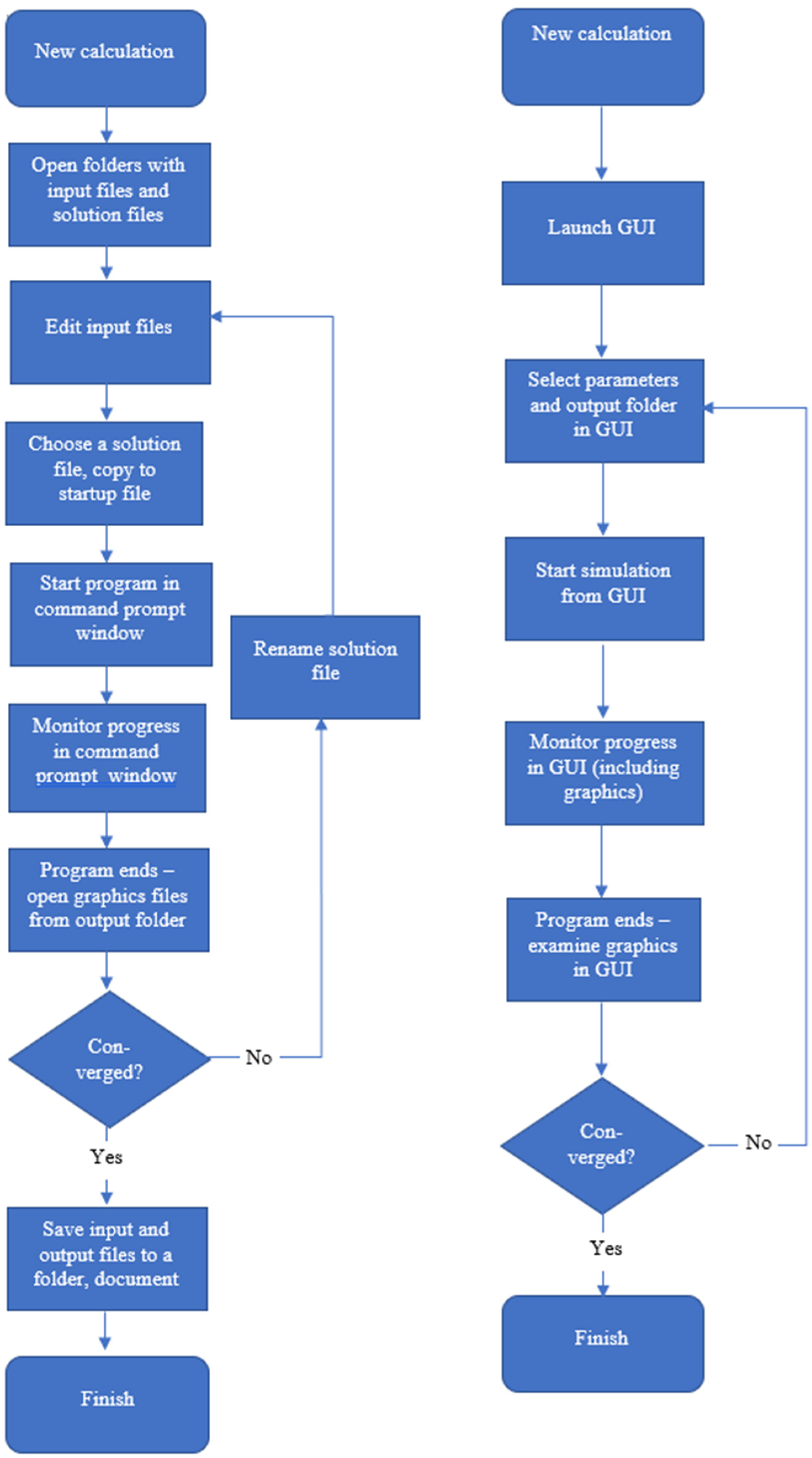
2.2. The Workflow before Refactoring

When the computer code was first developed, it was run on a desktop computer or workstation from the command prompt in the Windows operating system or the command line in a Unix operating system. Figure 3 (left-hand side) presents a flow diagram that outlines the operation of the code.
Before running the code, three text files defining the input parameters had to be edited manually. The files contained, respectively:
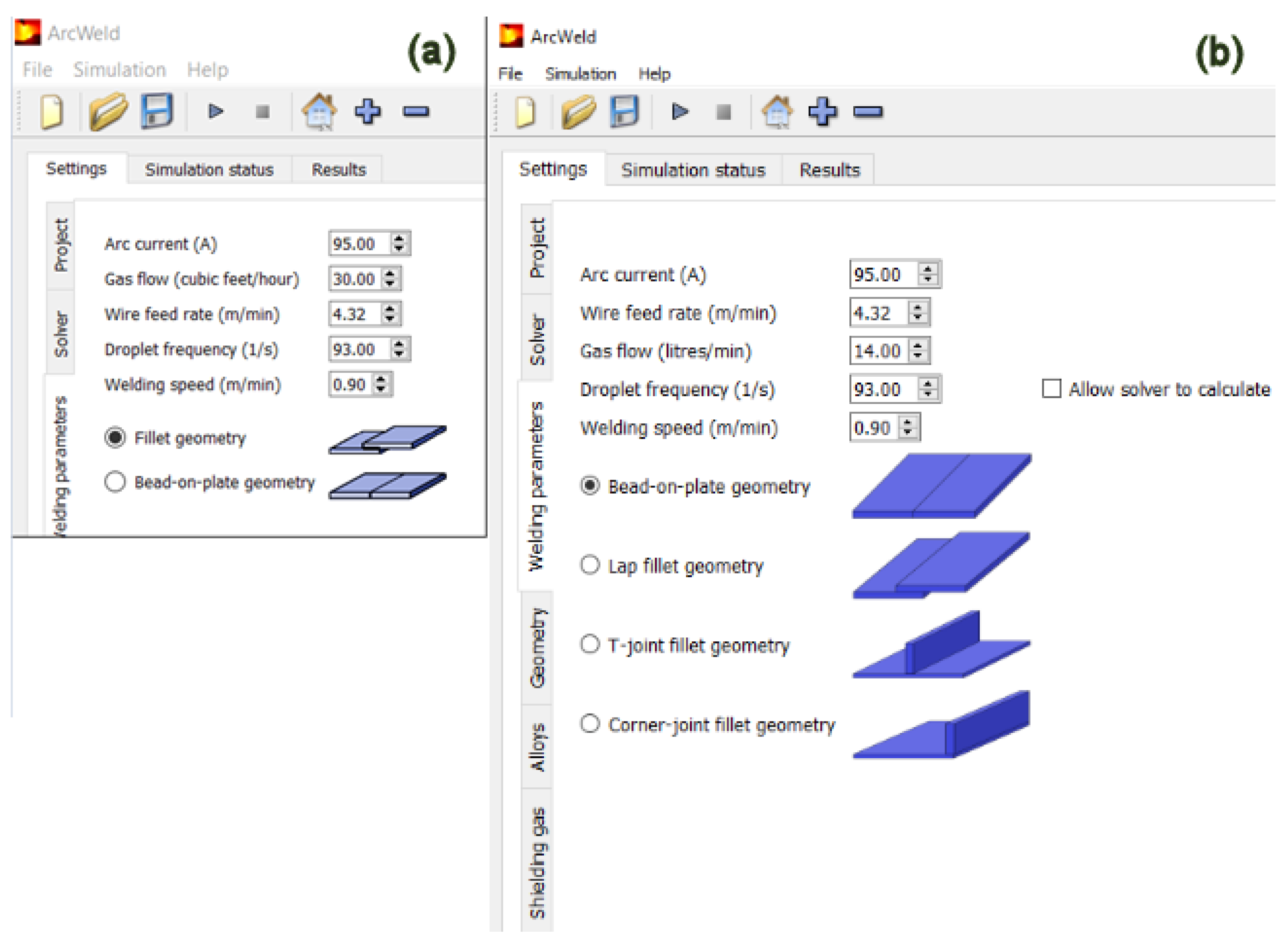
  • The welding parameters (such as arc current, welding speed, and wire feed rate), factors that control the computation (e.g., the maximum number of iterations, the convergence criteria, and relaxation factors), and options (e.g., type of workpiece geometry, whether to use a previous solution file or calculate an approximate solution, and whether to consider the mixing of the wire and workpiece alloys);
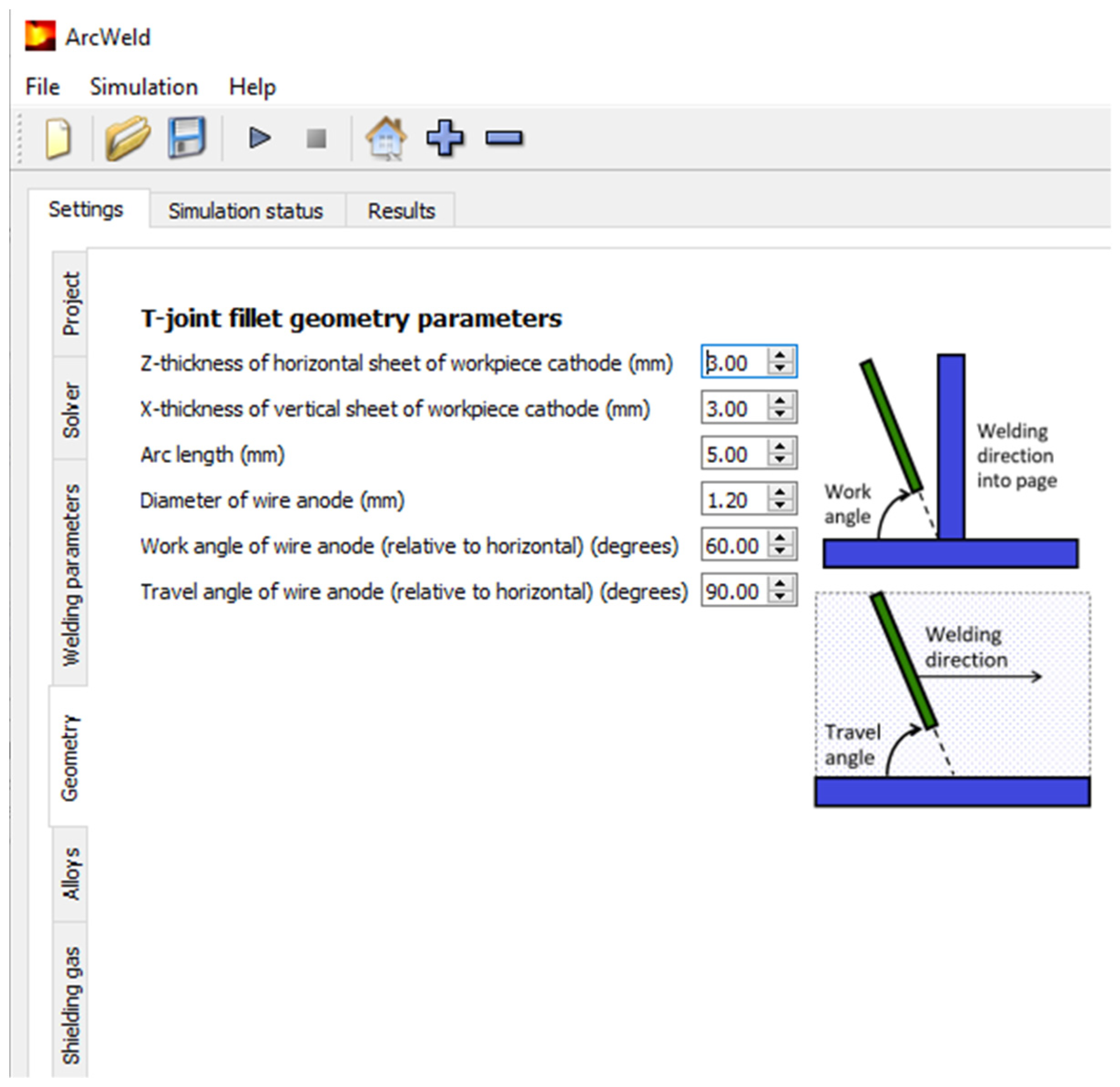
  • The geometric parameters (the diameter and orientation of the wire, the arc length, the thickness of the workpiece sheets, the dimensions of the computational domain, etc.), and meshing parameters (the number of control volumes in different regions, etc.); separate files were used for each geometry;
  • The metal alloys used for the wire and workpiece; alternatively, the elemental composition could be specified.
The code created an output text file that lists, for every control volume, the temperature, electric potential, magnetic potential, metal vapour concentration, wire alloy concentration, and components of the velocity, current density, and magnetic potential vectors. If the run was to be initiated using a previous solution file, then the appropriate file had to be manually selected from a library containing files corresponding to previous solutions, which may have been fully or only partially converged. Once the solution file was located, it had to be copied manually to the folder containing the input parameter text files and renamed so that the code could recognise it. Alternatively, the code could be run ‘from scratch’; in this case, the code calculated an approximate initial solution. The code was run from a command prompt. Text output showing progress towards convergence and other data was written to the screen. Following each iteration, the code wrote several output files, including diagnostic information and binary graphics files in Tecplot format. A solution file was written after the final iteration.
There was ample scope for user error at each manual stage of this process. For example, incorrect parameters could be entered in the text file, the wrong input or solution files could be selected, and output files could be overwritten. Further, the user had to take care to record the parameters used in each run and save files to appropriate folders. Following this process required substantial training and experience; even experienced users sometimes encountered difficulties.

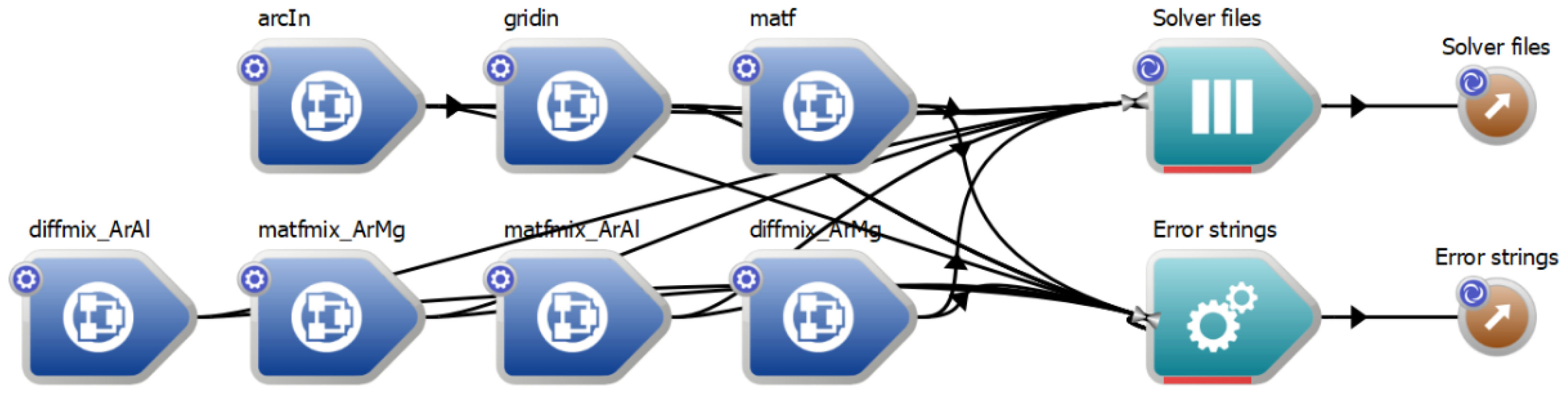
2.3. The Method Used for Refactoring

The application was constructed using the Workspace platform. Workspace is a scientific workflow system suited to many software development roles [18,43,44,45,46]. Its key component is the workflow, consisting of operations (representing discrete functional parts of a workflow) and connections between these operations (which transfer data between operations). Workflows can be nested, referenced externally, and linked to GUIs.
In the case of ArcWeld, Workspace was used to build a standalone compiled and installable Windows software application (see Ref. [47] for more details on using Workspace as a tool to improve modelling and simulation processes). The approach was to automate all the problematic and error-prone manual tasks mentioned in Section 2.2, enforce data validity, streamline the underlying process (e.g., manage input and output file locations on behalf of the user), integrate these with solver execution and monitoring, and provide easy access to the results. This was performed using Workspace workflows, Qt [48,49], and some custom C++ framework code.
The main workflow is shown in Figure 4. Its purpose is to read user entries in the GUI, translate them into input for the solver code, and then generate the files needed by the solver to run the simulation.
The dark blue operations on the left are all nested workflows—i.e., each one represents a workflow in its own right. These nested workflows generate the contents of each solver input file. The nested workflows are given the same name as the input file they generate. They read each data entry (e.g., arc current, the maximum number of iterations) from the GUI, convert the number to the units used in the solver, construct the data structure to be output (i.e., the file to be read by the solver), and pass the data and any error strings back to the parent workflow.
The central two light-blue operations collect the data generated by the previous operations. In this case, the uppermost operation collects all the files, and the lower one collects any reported errors or warnings, feeding this information back to the user via the GUI as required. The brown operations on the right are the outputs from this workflow. These are used by the code running this workflow—the outputs are monitored, and when complete and the user is ready to run the simulation, the files are written to disk, and the monitoring of the solver process begins. A detailed description of the workflows and their implementation in Workspace was given previously [19].
An important benefit of using a workflow structure is the ability to extend and modify the software. For example, the original version of ArcWeld was developed for the welding of aluminium alloy sheets in bead-on-plate and lap fillet geometries, which are illustrated in Figure 5a.
In a subsequent project, jointly funded by the Rail Manufacturing Cooperative Research Centre (RMCRC) and CRRC Qishuyan Locomotive & Rolling Stock Technology Research Institute Co., Ltd., Qishuyan, China (CRRC QSYRI), four main extensions to the capability of the ArcWeld software were requested:
  • Inclusion of additional metals, including Al-Mg-Zn alloys, magnesium alloys, mild steels, and carbon steels;
  • Inclusion of shielding gases composed of Ar-O2 and Ar-CO2 mixtures, which are widely used in the welding of steels;
  • Inclusion of two additional welding geometries, T-joint and corner-joint (or fillet) weld geometries;
  • Inclusion of built-in graphics.
Each of the first three changes, particularly the third, required significant changes to the FORTRAN code. These changes were easily integrated into ArcWeld software with the addition of new workflow elements. An example is shown in Figure 4. The solver required additional input files matfmix_ArMg and diffmix_ArMg containing plasma property data for mixtures of argon and magnesium vapour. New nested workflows of the same names were introduced. Note that additional nested workflows for steel and Ar-O2 and Ar-CO2 mixtures have been omitted from Figure 4 for the sake of clarity.
It was similarly straightforward to update the GUI, as shown in the example given in Figure 5. The two additional geometries were added to the ‘Welding parameters’ screen. The options displayed in the ‘Geometry’ screen depend on the geometry selected.
The last change in the second version of ArcWeld was the inclusion of graphics integrated into the GUI. The commercial Tecplot graphics software was relied on in the first version to save development costs. The solver wrote output binary files in a format readable by Tecplot, and the GUI provided a simple interface to launch Tecplot with the relevant file opened.
  • Including graphics in an application typically requires a large investment. In this case, however, a new Advanced Charting plugin from the Workspace ecosystem was available. The change was obviously not as trivial as the matfmix file update discussed above. Nevertheless, it was relatively simple, as the following outline of the main steps illustrates. The Fortran code in the solver was modified to output the results in an easy-to-parse Workspace-friendly data format, which could be ASCII or binary.
  • New Workspace operations were written to read each of the output files. The Workspace editor’s wizards facilitated the creation of the necessary stub code, with the developer adding the required functionality by parsing the data output by the solver and populating one of Workspace’s built-in data types.
  • The data output from the new read operations was connected to a CreateChart operation. This operation provides various configurations for titles, labelling, etc.
  • A new widget, a Workspace-supplied ChartWidget, was added to the GUI via Qt Designer [48], which allows for simple drag and drop of graphical components.
  • The workflow chart element was connected to the GUI chart widget. The workflow chart element is an output containing the chart data created by the CreateChart operation. Connecting these two items simply required the developer to drag from the workflow (in the Workspace editor) to the chart widget (in Qt Designer) [48]. This demonstrates an important benefit of using the Workspace environment—the ease of connecting GUI and workflow components.

3. Results

The refactoring of the code and its integration into the Workspace platform led to significant improvements in the workflow, which we describe in this section.
The GUI controls all aspects of code operation, as shown by the flow diagram in Figure 3 (right-hand side). The GUI contains six input screens under the ‘Settings’ tab, respectively headed ‘Project’, ‘Solver’, ‘Welding parameters’, ‘Geometry’, ‘Alloys’, and ‘Shielding gas’. Two examples are given here: the ‘Welding parameters’ window shown in Figure 5 and the ‘Geometry’ window shown in Figure 6. The available process parameters are given in Table 2. The choice of many of the parameters, including the alloys and shielding gases, were determined based on customer requirements.
Standard features such as a menu and toolbar are also available, incorporating components common in the vast majority of modern applications; these are shown in Figure 6.
After the code is started, the status of the simulation (the number of iterations and progress towards convergence) is shown on a colour-coded screen, viewable by selecting the ‘Simulation status’ tab on the main navigation bar (the collection of three horizontal tab labels—‘Settings’, ‘Simulation status’, and ‘Results’, visible in Figure 6).
The ‘Results’ tab can be viewed at any time. Three main choices are available:
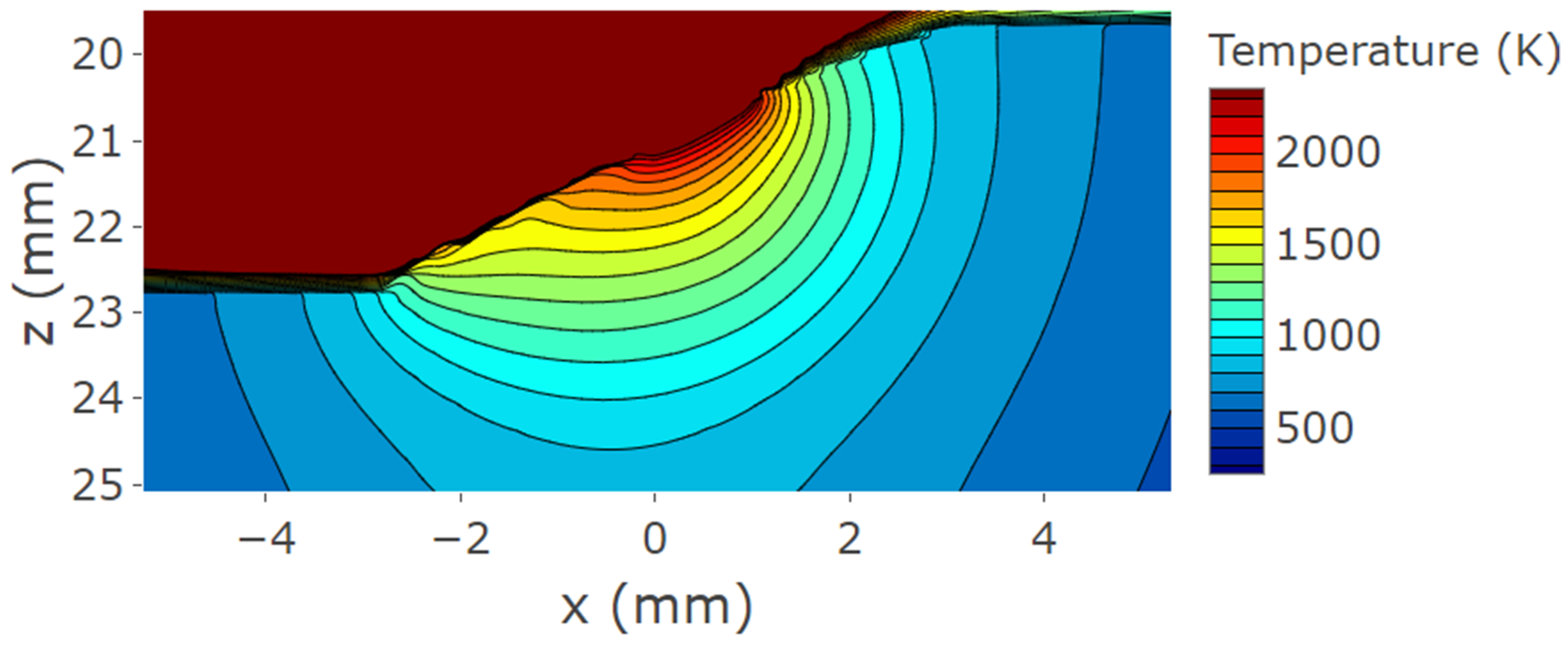
  • ‘Slice views of weld in progress’, which provides two-dimensional contour plots in the x-y, y-z, and x-z planes (where the z-axis is vertical, and the x-axis and y-axis are in the horizontal plane, with the y-axis aligned with the weld direction). Many properties can be viewed, including temperature, flow speed and its components, current density components, electric potential, mass fraction of metal vapour in the arc, and wire alloy mass fraction in the workpiece.
  • ‘Surface view of the weld in progress’, which provides two-dimensional contour plots, viewed from above, of the height of the weld, temperature of the workpiece surface, and the arc pressure and droplet pressure on the workpiece surface.
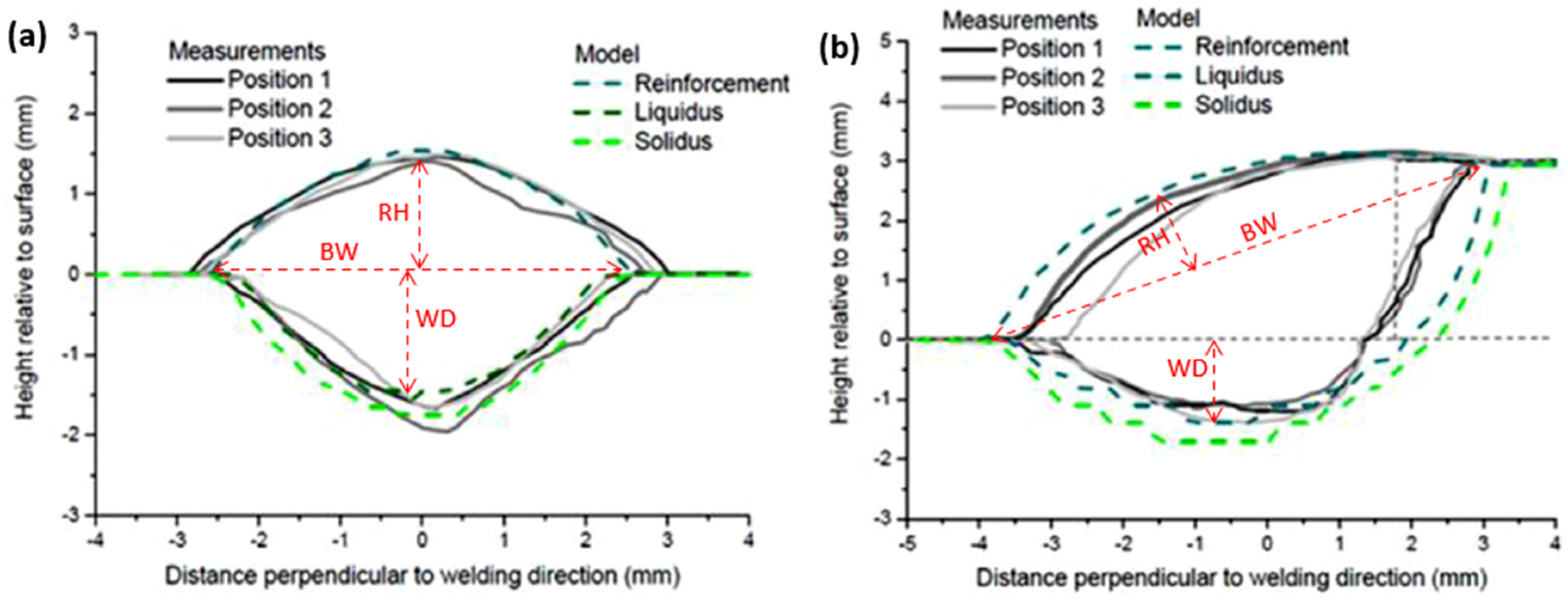
  • ‘Weld cross-section after welding’, which gives a line plot representation of the weld cross-section, including heat-affected zones.
Examples of the three main plots are shown in Figure 7. The user can zoom in on regions of interest in the contour plots and change the scale as required. An example, showing a more detailed view of temperature distribution in the weld pool and surrounding regions, is shown in Figure 8.
A folder whose name and location are entered in the GUI by the user is created before starting the code. A project file (containing all necessary data to represent the simulation in the GUI) and the input files (i.e., the text files and solution file read by the code) are written to this folder. The GUI does not change the code execution. All output files are written to the folder. The user does not need to be aware of these files, only the location of their project. The project file can be shared with other users.

4. Discussion

In this section, we discuss the improved simulation practice that has resulted from the building of the software as a Workspace application.
The previous implementation of the code had significant drawbacks:
  • The input files had to be modified manually whenever the welding or other parameters were altered. This task required the user to have a detailed knowledge of the format of the input files, avoid any typing errors, and ensure that erroneous parameter values were not entered. Moreover, the input file format was often changed when the code was modified, so reusing old input files frequently required them to be edited. No restrictions were imposed on the values of the parameters that could be entered. This meant that incorrect or incompatible values could only be identified by running the code, adding overhead to the running of the solver code and sometimes wasting considerable time if the error was not picked up.
  • The input files and output files were saved to a default folder. The user was responsible for documenting the input parameters and results and manually managing the input and output file storage. This requirement makes user errors (e.g., looking in the wrong location, accidental overwriting of files) much more likely, and considerable care is required to avoid such problems. The GUI application handles the management of files, removing the need for such user intervention and vigilance.
  • The user had to choose the solution file used for the initial solution estimate. After selecting the appropriate file, the user moved it manually to the input file folder and renamed it. As discussed below, the GUI application automates this process while retaining user freedom.
  • The screen display of the progress of the model towards convergence was non-intuitive, consisting only of text, and required detailed understanding to interpret. The GUI application displays the progress in a separate window using an intuitive colour-coded display.
  • The user had to open the output text and graphics files from the default folder, requiring knowledge and maintenance of the file locations. The GUI application provides a selection of graphics, which are updated after every iteration, in a separate window.
A common feature of the previous code implementation, which is typical of many research codes, is that documentation and file storage depend on the user’s work practices. Substantial variation occurs between users, and the practices of a particular user may change depending on work pressures. Accordingly, documentation and file storage were very uneven. Other problems included user error in file editing and location management and a lack of reproducibility in the workflow of setting up, running, viewing, and storing the results of a simulation.
The refactoring of the software to use Workspace and the integration of the code with the GUI automated the operation of the workflows required for code execution. For example, a common problem noted above was selecting and implementing the solution file used for an initial solution estimate. In the refactored software, the appropriate solution file is automatically selected from a library based on the parameters entered into the GUI. Alternatively, the user can use the solution file from the previous run or have the code calculate the initial solution. The user no longer has to copy or rename previous solution files, eliminating a common source of error. As a second example, all parameters and files associated with a run are stored in a single folder. Thus, the user only has to name the folder; the only documentation required is to associate the name with any required information. The complete automation of the workflow enforces a helpful level of user discipline and reduces the level of demand on the user to make good workflow practice decisions, both of which contribute to improved modelling practice.
Several other factors have been built into the GUI to ensure increased reliability and ease of use.
  • Preselected default values for all parameters are given for various configurations;
  • Selected parameters are required to fall within the range for which the code has been tested;
  • The validity of all other parameters (including those that may interact with each other) is ensured by rules built into the GUI;
  • Monitoring the progress of the code is much more intuitive;
  • Viewing of results is greatly simplified by the inbuilt graphics.
The Workspace-integrated code has significant benefits, even for the expert user. The user no longer has to worry about details of the code, storage locations, and documentation, with a consequent reduction in errors. Instead, they are freed to concentrate on generating research results, increasing productivity. New users can run the code with minimal training. Existing users who have not run the code for an extended period can easily recommence work without spending time reviewing documentation and input file formats and locations, allowing useful simulations to be performed in even short periods of available time. Transfer of the software between researchers is also much easier, and the standardised set of output files facilitates the comparison of results.
A notional penalty associated with refactoring the software might be a perceived reduction in flexibility. For example, the user may wish to increase the range of an input parameter or add more options to the list of possible alloys. However, it is simple to update the application using existing Workspace tools, as shown by the examples given in Section 2.3. Editing the FORTRAN code is usually necessary, but this is a common feature of the original and new implementations. The modifications to the GUI do require a little additional work, but these are documented and clearly visible to the user. Moreover, if necessary, the user can edit the input files by hand before running the solver. We have found that the advantages greatly outweigh any drawbacks. Research productivity has improved, and the results obtained are more reliable and better documented.
A significant advantage of this approach is that non-experts can readily run the code. All that is required is brief training (using, for example, the tutorial files provided with the software), a basic knowledge of Windows, and access to a standard desktop or laptop computer. Welding engineers and technicians rarely have the skills or time to run a ‘research’ code, nor do they have access to specialised computer facilities. However, they generally use desktop computers and Windows routinely. Consequently, the software can be used ‘on the factory floor’ alongside practical testing to improve and optimise welding processes. This is particularly important for welding alloys with which the welders have limited or no experience. Trial and error efforts to determine appropriate welding parameters are time-consuming, since they typically require the welded metal to be sectioned and polished to examine the weld cross-section. ArcWeld predicts these cross-sections and allows for the influence of different welding parameters to be determined. The software also allows for the welding professional seeking a deeper understanding of the process to visualise phenomena such as the flow in the weld pool, which contribute to the success of the weld. Examples of the application of the software in solving welding problems have been presented elsewhere [42]. These factors also mean the software is suitable for training welding technicians and engineers. Moreover, the software is easy to demonstrate to potential customers, which has increased the attractiveness and visibility of our arc plasma modelling work to a range of companies.
The welding process parameters treated by ArcWeld, listed in Table 2, were defined by client requirements. The range of parameters can be extended in the future in line with the request of clients and researchers. For example, additional shielding gas mixtures and wire and workpiece alloys could easily be included. The extension would require straightforward modifications to the solver and GUI; for example, the inclusion of new matfmix and diffmix files that provide thermophysical data for the new shielding gases, as discussed in Section 2.3.
ArcWeld provides predictions of the weld geometry and composition of the weld and detailed information about the distributions of temperature, flow velocities, and other quantities in the workpiece and arc. However, the prediction of important parameters, such as metal microstructure and residual stress evolution, is beyond the capabilities of CFD software. ArcWeld can be coupled with FEA software to help address this issue. Initial efforts involved coupling the thermal histories of the workpiece predicted by ArcWeld to commercial FEA software, which was used to predict residual stress and distortion [33]. We are currently working on a different approach in which the arc heat flux predicted by ArcWeld is used as the input for commercial FEA software. This approach is being applied to wire-arc additive manufacturing, which uses arc welding technology to ‘print’ large metal components layer by layer [50]. By itself, ArcWeld is not well suited to modelling wire-arc additive manufacturing for two main reasons. First, it is limited to relatively small components to keep computational time within reasonable limits. Second, it runs in steady-state mode, reducing its accuracy when applied to the deposition of multiple layers, since the cooling of previous layers during deposition of a new layer cannot be handled. FEA software is capable of time-dependent modelling of the deposition of many layers to produce large components. However, as noted in Section 1, it relies on estimates of the heat flux from the arc, which require experimental calibration. By coupling the heat flux predicted by ArcWeld to FEA software, the evolution of residual stress and distortion in large components can be predicted without the need for experiments to calibrate the estimated heat source.

5. Conclusions

As with many areas of research, computational modelling of thermal plasma and other plasma processes is of major importance in plasma process research and development. Modelling has always provided scientific insights and helped explain experimental results. In recent years, the modelling of plasma processes has become sufficiently sophisticated to be applied to process development and improvement, including in industry.
Many computer codes for plasma modelling have been developed by researchers, as discussed in Section 1. Very often, however, the code is written as a research tool. As we have discussed, this decreases convenience and increases the likelihood of errors. Moreover, there is a high risk of the knowledge required to run the code being lost, for example, if the researcher responsible for maintaining the code leaves. Refactoring the code into a software package with an intuitive GUI greatly mitigates this risk, particularly if instructions and tutorials are packaged with the software. We have presented a detailed example of the transformation of a research code for the modelling of arc welding into a software product.
The refactoring and integration of the arc welding computer code with an intuitive, easy-to-use GUI and the complete automation of the supporting workflow using the Workspace workflow platform have had substantial benefits. These have accrued both for users (research and commercial) and for the developer of the solver itself.
The commercialisation of the intellectual property embedded in the solver was made feasible at a low cost by the ease of use of Workspace and Qt Designer to create the application. These tools facilitated a modular approach, with nested workflows used to ensure easy construction and visualisation of the overall workflow. The modularity enabled the extension of the software to accommodate additional capabilities. Users are presented with all the usual familiar GUI components—menu, toolbar, easy access to documentation, etc. Such an interface is a significant advantage when commercialisation is a goal, allowing purchasers to be confident that the interface will help rather than hinder their engineers and technicians on the shop floor. It also presents a much easier learning curve, allowing users to get up to speed much more quickly, having to understand only technical information relevant to the simulation rather than how to run it.
The approach is readily transferrable to research codes developed for the modelling of manufacturing and other processes. Only limited modifications are required to the research code. The main requirement is a collaboration with a software engineer with access to the required tools. The development of the ArcWeld application has dramatically increased the accessibility of the code. It can now be used by welding engineers and technicians in an industrial environment, is suitable for the training of welders, and can be promoted to potential customers. Without this development, such outreach would have been close to impossible.

Author Contributions

Conceptualisation, A.B.M. and D.G.T.; methodology, A.B.M., D.G.T., F.F.C., and Y.F.; software, A.B.M., D.G.T., F.F.C., J.X. and Y.F.; validation, A.B.M. and F.F.C.; investigation, A.B.M., D.G.T., F.F.C. and J.X.; writing—original draft preparation, A.B.M. and D.G.T.; writing—review and editing, A.B.M., D.G.T., F.F.C., J.X. and Y.F., visualisation, A.B.M. and D.G.T.; supervision, A.B.M.; project administration, A.B.M.; funding acquisition, A.B.M. All authors have read and agreed to the published version of the manuscript.

Funding

The support provided for the work reported here by General Motors, General Motors Holden, and the Commonwealth of Australia, through the AutoCRC, and the financial support from the Rail Manufacturing Cooperative Research Centre (funded jointly by participating rail organisations and the Australian Federal Government’s Business Cooperative Research Centres Program) is gratefully acknowledged.

Institutional Review Board Statement

Not applicable.

Informed Consent Statement

Not applicable.

Data Availability Statement

Not applicable.

Acknowledgments

Damien Watkins, Paul Cleary, John Lowke, and Eugene Tam of CSIRO, Hui-Ping Wang of General Motors, and Jiaqi Gu of CRRC QSYRI are thanked for valuable discussions. The work presented here is partially based on papers published in the Proceedings of the 22nd and 23rd International Congresses on Modelling and Simulation [19,20].

Conflicts of Interest

The authors declare no conflict of interest. The funders had no role in the design of the study; in the collection, analyses, or interpretation of data; in the writing of the manuscript, or in the decision to publish the results.

References

  1. Zielinska, S.; Musiol, K.; Dzierzega, K.; Pellerin, S.; Valensi, F.; de Izarra, C.; Briand, F. Investigations of GMAW plasma by optical emission spectroscopy. Plasma Sources Sci. Technol. 2007, 16, 832–838. [Google Scholar] [CrossRef]
  2. Rouffet, M.E.; Wendt, M.; Goett, G.; Kozakov, R.; Schoepp, H.; Weltmann, K.D.; Uhrlandt, D. Spectroscopic investigation of the high-current phase of a pulsed GMAW process. J. Phys. D Appl. Phys. 2010, 43, 434003. [Google Scholar] [CrossRef]
  3. Kozakov, R.; Gött, G.; Schöpp, H.; Uhrlandt, D.; Schnick, M.; Hässler, M.; Füssel, U.; Rose, S. Spatial structure of the arc in a pulsed GMAW process. J. Phys. D Appl. Phys. 2013, 46, 224001. [Google Scholar] [CrossRef]
  4. Kühn-Kauffeldt, M.; Marqués, J.-L.; Schein, J. Thomson scattering diagnostics of steady state and pulsed welding processes without and with metal vapor. J. Phys. D Appl. Phys. 2015, 48, 012001. [Google Scholar] [CrossRef]
  5. Haddad, G.N.; Farmer, A.J.D. Temperature determinations in a free-burning arc. I. Experimental techniques and results in argon. J. Phys. D Appl. Phys. 1984, 17, 1189–1196. [Google Scholar] [CrossRef]
  6. Farmer, A.J.D.; Haddad, G.N.; Cram, L.E. Temperature determinations in a free-burning arc: III. Measurements with molten anodes. J. Phys. D Appl. Phys. 1986, 19, 1723–1730. [Google Scholar] [CrossRef]
  7. Boulos, M.I.; Fauchais, P.; Pfender, E. Thermal Plasmas: Fundamentals and Applications; Plenum: New York, NY, USA, 1994; Volume 1. [Google Scholar]
  8. Murphy, A.B.; Uhrlandt, D. Foundations of high-pressure thermal plasmas. Plasma Sources Sci. Technol. 2018, 27, 063001. [Google Scholar] [CrossRef]
  9. Gleizes, A.; Gonzalez, J.J.; Freton, P. Thermal plasma modelling. J. Phys. D Appl. Phys. 2005, 38, R153–R183. [Google Scholar] [CrossRef]
  10. Furukawa, R.; Tanaka, Y.; Nakano, Y.; Nagase, Y.; Ishijima, T.; Sueyasu, S.; Watanabe, S.; Nakamura, K. Numerical study of nanoparticle formation in two-coil tandem-type modulated induction thermal plasmas with simultaneous modulation of upper- and lower-coil currents. J. Phys. D Appl. Phys. 2021, 55, 044001. [Google Scholar] [CrossRef]
  11. Shigeta, M.; Watanabe, T. Growth model of binary alloy nanopowders for thermal plasma synthesis. J. Appl. Phys. 2010, 108, 043306. [Google Scholar] [CrossRef]
  12. Girshick, S.L.; Chiu, C.-P.; McMurry, P.H. Modelling particle formation and growth in a plasma synthesis reactor. Plasma Chem. Plasma Process. 1988, 8, 145–156. [Google Scholar] [CrossRef]
  13. Shigeta, M. Turbulence modelling of thermal plasma flows. J. Phys. D Appl. Phys. 2016, 49, 493001. [Google Scholar] [CrossRef]
  14. Jenista, J.; Chau, S.-W.; Chen, S.-W.; Zivny, O.; Takana, H.; Nishiyama, H.; Bartlova, M.; Aubrecht, V.; Murphy, A.B. Modelling of argon–steam thermal plasma flow for abatement of fluorinated compounds. J. Phys. D Appl. Phys. 2022, 55, 375201. [Google Scholar] [CrossRef]
  15. Agarwal, A.; Bera, K.; Kenney, J.; Likhanskii, A.; Rauf, S. Modeling of low pressure plasma sources for microelectronics fabrication. J. Phys. D Appl. Phys. 2017, 50, 424001. [Google Scholar] [CrossRef]
  16. Kushner, M.J. Hybrid modelling of low temperature plasmas for fundamental investigations and equipment design. J. Phys. D Appl. Phys. 2009, 42, 194013. [Google Scholar] [CrossRef]
  17. Xiong, X.; Kushner, M.J. Surface corona-bar discharges for production of pre-ionizing UV light for pulsed high-pressure plasmas. J. Phys. D Appl. Phys. 2010, 53, 505204. [Google Scholar] [CrossRef]
  18. CSIRO. Workspace; CSIRO: Canberra, Australia, 2018. [Google Scholar]
  19. Murphy, A.B.; Thomas, D.G. A computational model of arc welding—From a research tool to a software product. In Proceedings of the 22nd International Congress on Modelling and Simulation, Hobart, Australia, 3–8 December 2017; pp. 445–451. [Google Scholar]
  20. Thomas, D.G.; Murphy, A.B.; Chen, F.F.; Xiang, J.; Feng, Y. ArcWeld: A case study of the extensibility of software applications built using Workspace architecture. In Proceedings of the 23rd International Congress on Modelling and Simulation, Canberra, Australia, 1–6 December 2019; pp. 470–476. [Google Scholar]
  21. ESI Group. SYSWELD. Available online: https://www.esi-group.com/products/sysweld (accessed on 12 April 2023).
  22. Flow Science. FLOW-3D. Available online: https://www.flow3d.com/ (accessed on 12 April 2023).
  23. Cao, Z.; Yang, Z.; Chen, X.L. Three-dimensional simulation of transient GMA weld pool with free surface. Weld. J. 2004, 83, 169s–174s. [Google Scholar]
  24. Flow Science. FLOW-3D Weld. Available online: https://www.flow3d.com/products/flow3d-weld/ (accessed on 12 April 2023).
  25. Goldak, J.; Chakravarti, A.; Bibby, M. A new finite element model for welding heat sources. Metall. Trans. B 1984, 15B, 299–305. [Google Scholar]
  26. Yang, Z.; Elmer, J.W.; Wong, J.; DebRoy, T. Evolution of titanium arc weldment macro and microstructures modeling and real time mapping of phases. Weld. J. 2000, 79, 97s–112s. [Google Scholar]
  27. Aryal, P.; Sikström, F.; Nilsson, H.; Choquet, I. Comparative study of the main electromagnetic models applied to melt pool prediction with gas metal arc: Effect on flow, ripples from drop impact, and geometry. Int. J. Heat Mass. Transf. 2022, 194, 123068. [Google Scholar] [CrossRef]
  28. Cleary, P.; Hetherton, L.; Bolger, M.; Rucinski, C.; Sankaranarayanan, N.; Thomas, D.; Watkins, D.; Zhang, Z.; Subramanian, R.; Nguyen, D.Q.; et al. Workspace: Scientific Workflow Platform; CSIRO: Canberra, Australia, 2017. [Google Scholar]
  29. Norrish, J. Advanced Welding Processes; Institute of Physics Publishing: Bristol, UK, 1992. [Google Scholar]
  30. Murphy, A.B. The effects of metal vapour in arc welding. J. Phys. D Appl. Phys. 2010, 43, 434001. [Google Scholar] [CrossRef]
  31. Murphy, A.B. A self-consistent three-dimensional model of the arc, electrode and weld pool in gas–metal arc welding. J. Phys. D Appl. Phys. 2011, 44, 194009. [Google Scholar] [CrossRef]
  32. Murphy, A.B. Influence of metal vapour on arc temperatures in gas–metal arc welding: Convection versus radiation. J. Phys. D Appl. Phys. 2013, 46, 224004. [Google Scholar] [CrossRef]
  33. Murphy, A.B.; Nguyen, V.; Feng, Y.; Thomas, D.G.; Gunasegaram, D. A desktop computer model of the arc, weld pool and workpiece in metal inert gas welding. Appl. Math. Model. 2017, 44, 91–106. [Google Scholar] [CrossRef]
  34. Murphy, A.B.; Chen, F.F.; Xiang, J.; Wang, H.-P.; Thomas, D.G.; Feng, Y. Macrosegregation in the weld pool in metal inert-gas welding of aluminium. J. Manuf. Process. 2021, 61, 111–127. [Google Scholar] [CrossRef]
  35. Patankar, S.V. Numerical Heat Transfer and Fluid Flow; Hemisphere: Washington, DC, USA, 1980. [Google Scholar]
  36. Lowke, J.J.; Kovitya, P.; Schmidt, H.P. Theory of free-burning arc columns including the influence of the cathode. J. Phys. D Appl. Phys. 1992, 25, 1600–1606. [Google Scholar] [CrossRef]
  37. Crowe, C.T.; Sharma, M.P.; Stock, D.E. The particle-source-in cell (PSI-CELL) model for gas-droplet flows. J. Fluid Eng. 1977, 99, 325–332. [Google Scholar] [CrossRef]
  38. Murphy, A.B. Influence of droplets in gas–metal arc welding—A new modelling approach, and application to welding of aluminium. Sci. Technol. Weld. Join. 2013, 18, 32–37. [Google Scholar] [CrossRef]
  39. Hirt, C.W.; Nichols, B.D. Volume of fluid (VOF) method for the dynamics of free boundaries. J. Comput. Phys. 1981, 39, 201–225. [Google Scholar] [CrossRef]
  40. Mundra, K.; DebRoy, T.; Kelkar, K.M. Numerical prediction of fluid flow and heat transfer in welding with a moving heat source. Numer. Heat Transf. A 1996, 29, 115–129. [Google Scholar] [CrossRef]
  41. Lowke, J.J.; Tanaka, M. ‘LTE-diffusion approximation’ for arc calculations. J. Phys. D Appl. Phys. 2006, 39, 3634–3643. [Google Scholar] [CrossRef]
  42. Chen, F.F.; Xiang, J.; Thomas, D.G.; Murphy, A.B. Model-based parameter optimization for arc welding process simulation. Appl. Math. Model. 2020, 81, 386–400. [Google Scholar] [CrossRef]
  43. Bolger, M.; Cleary, P.; Hetherton, L.; Rucinski, C.; Thomas, D.; Watkins, D. Workspace: Scientific Workflow Platform; CSIRO: Canberra, Australia, 2014. [Google Scholar]
  44. Cleary, P.; Bolger, M.; Hetherton, L.; Rucinski, C.; Thomas, D.; Watkins, D. Workspace: A platform for delivering scientific applications. In Proceedings of the eResearch Australasia, Melbourne, Australia, 27–31 October 2014. [Google Scholar]
  45. Bolger, M.; Cleary, P.; Hetherton, L.; Rucinski, C.; Thomas, D.; Watkins, D. Workspace: Scientific workflows and applications for multiple environments. In Proceedings of the eResearch Australasia Conference, Brisbane, Australia, 19–23 October 2015. [Google Scholar]
  46. Cleary, P.W.; Thomas, D.; Bolger, M.; Hetherton, L.; Rucinski, C.; Watkins, D. Using Workspace to automate workflow processes for modelling and simulation in engineering. In Proceedings of the MODSIM2015, 21st International Congress on Modelling and Simulation, Gold Coast, Australia, 29 November–4 December 2015; pp. 669–675. [Google Scholar]
  47. Cleary, P.W.; Thomas, D.; Hetherton, L.; Bolger, M.; Hilton, J.E.; Watkins, D. Workspace: A workflow platform for supporting development and deployment of modelling and simulation. Math. Comp. Simul. 2018; submitted. [Google Scholar]
  48. The Qt Company Ltd. Qt Designer; The Qt Company Ltd.: Espoo, Finland, 2018. [Google Scholar]
  49. The Qt Company Ltd. Qt Property System; The Qt Company Ltd.: Espoo, Finland, 2018. [Google Scholar]
  50. Norrish, J.; Polden, J.; Richardson, I. A review of wire arc additive manufacturing: Development, principles, process physics, implementation and current status. J. Phys. D Appl. Phys. 2021, 54, 473001. [Google Scholar] [CrossRef]
Figure 1. Schematic of the MIG (metal inert gas) welding process. For MAG (metal active gas) welding, oxygen or carbon dioxide is added to the argon. © IOP Publishing. Reproduced with permission from [30]. All rights reserved.
Software 02 00012 g001
Figure 2. Comparison of the predicted weld cross section (reinforcement height, liquidus and solidus depths) with measured cross-sections at three locations along a weld of aluminium alloy AA5754 with an AA4043 wire for (a) bead-on-plate and (b) lap fillet weld geometries. The red dashed lines denote the weld dimensions used in Table 1. Adapted from [42] with permission from Elsevier.
Software 02 00012 g002
Figure 3. Two flow charts summarising the workflows for the code before (left) and after (right) integration with the GUI (graphical user interface) using Workspace. Adapted from [19].
Software 02 00012 g003
Figure 4. Main workflow for ArcWeld.
Software 02 00012 g004
Figure 5. (a) Version 1 and (b) version 2 of the ‘Welding parameters’ window in the ArcWeld GUI.
Software 02 00012 g005
Figure 6. Main GUI showing the ‘Geometry’ tab selected, following the choice of T-joint fillet geometry in the ‘Welding parameters’ tab. The images are included to clarify the definition of the work and travel angles.
Software 02 00012 g006
Figure 7. Representative figures viewable in the ‘Results’ tab: (a) the temperature field in a vertical cross-section, perpendicular to the welding direction, (b) the height of the reinforcement during a weld (viewed from above, with the weld progressing in the –y-direction), and (c) a weld cross-section. Welding parameters are for lap fillet geometry, with two 3 mm-thick AA4043 Al-Mg alloy workpiece sheets and a 1.2 mm-diameter AA4043 Al-Si alloy wire with work angle 60° and travel angle 90° from the horizontal. The arc current is 104 A, wire feed rate is 4.7 m s–1, and welding speed is 0.6 m min–1. The weld cross-section shows the reinforcement height (dark blue) and the regions that reached the liquidus temperature (light blue), solidus temperature (orange), a temperature of 400 °C (green), and a temperature of 300 °C (yellow); the horizontal axis is from –4 to 7 mm, and the vertical axis is from –3 to 4 mm.
Software 02 00012 g007
Figure 8. Zoomed-in and rescaled view of Figure 7a, showing details of the temperature field in the weld pool and surrounding regions of the workpiece.
Software 02 00012 g008
Table 1. Comparison of the weld dimensions predicted by the model (based on the liquidus location) with the measured dimensions (averaged over three locations).
RH (mm)WD (mm)BW (mm)
Bead-on-plateMeasured1.471.855.92
Predicted1.541.765.54
Lap filletMeasured1.261.427.12
Predicted1.421.678.15
Table 2. Process parameters selectable in the GUI.
ParameterAvailable Values
Arc current50–400 A
Gas flow0–20 L/min
Wire feed rate2.5–17 m/min
Droplet frequency10–200/s, or calculated by solver
Welding speed0.1–1.8 m/min
Workpiece geometryBead-on-plate, lap fillet, T-joint fillet, corner-joint fillet
Arc length2–10 mm
Wire diameter0.8–1.6 mm
Workpiece thickness2–30 mm; for lap, T-joint, and corner-joint fillet geometries, the thickness of each workpiece sheet can be specified independently.
Work angle of wire90° from horizontal for bead-on-plate; 45°, 60°, 75° for other geometries
Travel angle of wire90° from horizontal for bead-on-plate; 75°, 90° for other geometries
Workpiece alloyAl, user-defined Al-Si-Mg alloys with up to 15% Si and 5% Mg, user-defined Al-Mg-Zn alloys with up to 5% Mg and 5% Zn, user-defined steels with up to 2% C, 2% Si, 5% Mn, 30% Cr, 20% Ni, 5% Mo, 1% Ti, 1% V, 1% Al, 0.1% S, 0.1% P, and 0.1% N, AZ31 (an Mg-Al-Zn alloy), and several pre-defined Al-Si, Al-Mg, Al-Si-Mg, and Al-Mg-Zn alloys, low-alloy steels, and stainless steels
Wire alloyAs for workpiece alloys, with different pre-defined alloys based on standard wire materials
Shielding gas Ar, 98% Ar + 2% O2, 97.5% Ar + 2.5% CO2, 80% Ar + 20% CO2
Disclaimer/Publisher’s Note: The statements, opinions and data contained in all publications are solely those of the individual author(s) and contributor(s) and not of MDPI and/or the editor(s). MDPI and/or the editor(s) disclaim responsibility for any injury to people or property resulting from any ideas, methods, instructions or products referred to in the content.

