Article

AutodiDAQt: Simple Scientific Data Acquisition Software with Analysis-in-the-Loop

by
Conrad H. Stansbury
1,2 and
Alessandra Lanzara
1,2,3,*
1
Department of Physics, University California, Berkeley, CA 94720, USA
2
Materials Sciences Divisions, Lawrence Berkeley National Laboratory, Berkeley, CA 94720, USA
3
Center for Sustainable Materials and Innovation, Berkeley, CA 94720, USA
*
Author to whom correspondence should be addressed.
Software 2023, 2(1), 121-132; https://doi.org/10.3390/software2010005
Submission received: 7 December 2022 / Revised: 10 January 2023 / Accepted: 17 January 2023 / Published: 18 February 2023

Abstract

:
Scientific data acquisition is a problem domain that has been underserved by its computational tools despite the need to efficiently use hardware, to guarantee validity of the recorded data, and to rapidly test ideas by configuring experiments quickly and inexpensively. High-dimensional physical spectroscopies, such as angle-resolved photoemission spectroscopy, make these issues especially apparent because, while they use expensive instruments to record large data volumes, they require very little acquisition planning. The burden of writing data acquisition software falls to scientists, who are not typically trained to write maintainable software. In this paper, we introduce AutodiDAQt to address these shortfalls in the scientific ecosystem. To ground the discussion, we demonstrate its merits for angle-resolved photoemission spectroscopy and high bandwidth spectroscopies. AutodiDAQt addresses the essential needs for scientific data acquisition by providing simple concurrency, reproducibility, retrospection of the acquisition sequence, and automated user interface generation. Finally, we discuss how AutodiDAQt enables a future of highly efficient machine-learning-in-the-loop experiments and analysis-driven experiments without requiring data acquisition domain expertise by using analysis code for external data acquisition planning.

1. Introduction

The landscape of modern experimental physics is best conceived through the set of experimental tools that physicists use to interrogate space and matter. Historically, advances in instrumentation have been as significant as theoretical breakthroughs because the ability to perform new experiments allows scientists to pave over speculation with experimental proof. These advances are not always in hardware. Across techniques as diverse as ptychography [1], astrophysical imaging, cryo-electron microscopy [2,3], and various super-resolution and nonlinear microscopy techniques [4,5,6], instrumentation improvements require the integration of statistically sophisticated approaches to data analysis and acquisition. Over the last decade, analysis software tailored for individual experimental techniques has been a driving factor in bringing new analysis approaches into physical spectroscopies. In the domain of angle-resolved photoemission spectroscopy (ARPES) [7,8], the development of analysis and modeling toolkits such as PyARPES [9] and chinook [10], the integration of machine-learning-based denoising for ARPES spectra [11,12], and the continued development of new paradigms for the analysis of spectral data [13] all signal continued advances in the interpretation of high-dimensional spectroscopy. While these software packages ease the interpretation of data after data collection, they do not currently permit an effective use of acquisition hardware.
Because rapid innovation in ARPES experiments is still ongoing—most recently in the development of submicron resolution beams for photoemission [14,15,16] and the development of two-angle resolving time-of-flight electron analyzers [17,18,19]—this separation may remain because there is a belief that integrating more complex analysis is unnecessary for the time being. After all, nanoARPES is revolutionizing our understanding of two-dimensional materials [20], heterostructures [21,22,23,24,25], and electronic devices [26,27,28]. However, resolving the additional degrees of freedom in an experiment, as nanoARPES does by adding spatial resolution, usually makes contention for limited time on hardware worse and increases the demands on hardware apparatus for the efficient use of acquisition time. A minor reason for this is the greater demand for more capable experiments, but the real problem is fundamental: the curse of dimensionality means that experiments must record in sparser subsets of configuration space putting pressure on efficient use. The limited penetration of tightly integrated analysis and acquisition software in domains such as ARPES that might address this curse of dimensionality indicates friction and difficulty in tightly joining hardware and software. There are numerous benefits to be gained in more effectively using frequently limited acquisition time [29,30,31], removing sources of systematic bias from physical experiments, serving as checksums against common experimental and sample problems [32], and in allowing scientists to opt into collecting data driven by the statistical requirements of their analysis [33,34].
Scientists also actively interact with their data during an acquisition session by iteratively refining what they are measuring based on the data the experiment has yielded. Consequently, data acquisition is tightly integrated to a user interface (UI) controlling the acquisition session, to domain-specific data analysis tools, and to a large set of “application programming” concerns ranging from logging to data provenance. These are inviolable constraints for scientific data acquisition, but the burden they place explains the absence of universal approaches that more tightly integrate analysis, hardware, and software. It is vital to build software systems that allow scientists to restrict their attention to the issue of succinctly describing how hardware apparatus maps onto experimental degrees of freedom and sequencing data collection. Universal concerns—the thorny issues of user interfaces, data persistence, logging, error recovery, and data provenance—should be recycled because they are used across all scientific acquisition tasks. As things stand, most scientific DAQ software is purpose built to suit a given experiment with a vast amount of effort being spent on re-engineering solutions to the common concerns of the UI, persistence, and provenance. Because the exigency is for data, these concerns may not be addressed at all, especially in smaller university labs where DAQ software has usually evolved from existing LabVIEW VIs. When these issues are addressed, creating DAQ software may represent a substantial fraction of instrumentation effort and costs. Depending on the relative balance of hardware and personnel cost, DAQ engineering overheads may permit or inhibit novel experiments requiring synergistic combinations of hardware.
Here we present a new software system, AutodiDAQt, to address this problem space by providing a composable platform for describing DAQ systems. This new software system provides the necessary metaphors for tightly integrating scientific analysis and data acquisition and enabling analysis-in-the-loop and machine-learning-in-the-loop acquisition paradigms. This new system synthesizes the user interface and controls directly from the definitions of instrument drivers thereby reducing the problem of constructing scientific data acquisition software to the irreducible one of describing each instrument’s software interface and degrees of freedom. Because mature libraries and drivers for direct instrument control already exist [35,36,37,38], this reduces data acquisition software prototyping to a task that can be accomplished in a short period of time. Because it handles generating a user interface for instruments and for acquisition without end-user programming, AutodiDAQt is exceptionally well suited for writing DAQ software where scientists expect to be able to walk up to hardware and immediately start collecting data using the user interface, rather than by writing per experiment scan code.
Attempts to incorporate these needs in a flexible structure or to provide a general data acquisition framework for science [36,38,39,40,41,42], and to provide data acquisition systems serving a particular scientific discipline [33,34], have been adopted previously. For example, PyMeasure [35], a data acquisition framework for physics, provides user interface generation primitives for data acquisition but does not confront the problem of data provenance or make it straightforward to compose and refine acquisition sequences. Bluesky [43] and Auspex [38] capture the essentials of composing acquisition routines and offer robust support for metadata, but Bluesky requires a significant amount of configuration code and neither framework provides user interface generation to achieve the application fluency appropriate for setting up experiments quickly in small labs. The approach we advocate in AutodiDAQt is a simple, low-code approach incorporating the strengths of PyMeasure (strong user interface support) and Bluesky (strong composability). AutodiDAQt is designed to be appropriate for rapidly creating and modifying scientific experiments and reflects the need for small-scale, flexible experiments that can be adapted to rapid advances in both hardware and data analysis software. This is in strict contrast to systems such as Bluesky which, based on different philosophy, emphasize the ability to adopt pieces of the acquisition system “à la carte” and thereby require software engineering work to integrate into a full-fledged DAQ application. This can be seen as a focus for AutodiDAQt and a distinguishing characteristic in a robust landscape of data acquisition software: AutodiDAQt excels at providing full data acquisition applications by restricting its focus to user interface generation, experiment planning, and downstream application programming consequences such as data provenance. In the following sections, we outline the ways in which AutodiDAQt adopts and extends the strengths of acquisition user interfaces and program composability. In the final section, we discuss how AutodiDAQt permits the control of the acquisition software directly by live analysis and also the prospects for this paradigm in ARPES.

2. Materials and Methods

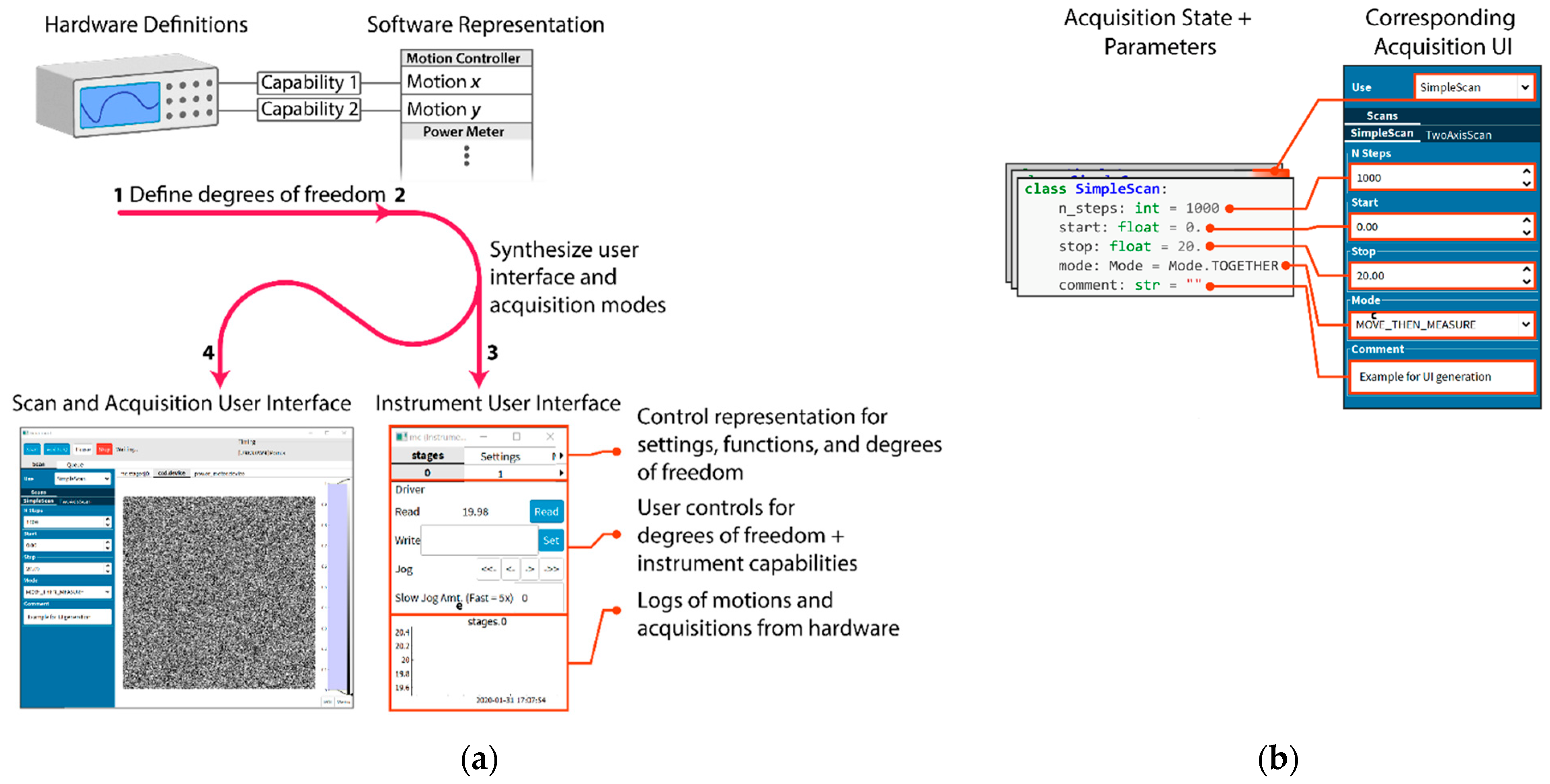
Relieving the burden of application programming from scientists requires automatically generating as much of the common user interface as is possible. AutodiDAQt leverages the highly structured nature of DAQ tasks to generate user interface (UI) elements for experiment parameters, collected values, data streams, and experimental apparatus. For this reason, AutodiDAQt uses schemas extending the Python-type system to provide control over data validation and data representation in the UI. At a coarser level, we recognize that writing DAQ software is an application programming task more than an algorithmic one and so provides high-level primitives for the UI that map onto application features where it is necessary or desirable to extend the default AutodiDAQt—for instance as the application needs to mature with an experiment. Experiment controls and acquisition interfaces are generated automatically (Figure 1(a3)) together within the acquisition session manager (Figure 1(a4)) just by defining the degrees of freedom in an experiment in terms of hardware capabilities exposed by instrument drivers (Figure 1(a1)). Most significantly, AutodiDAQt generates controls, streaming plots, and virtual front panels for hardware (Figure 1(a3)), obviating the need for UI programming, unless an experiment’s constraints are very unusual, through a combination of schema annotation and instrument driver specification. By defining these degrees of freedom, we will see in the following section that AutodiDAQt makes it straightforward to compose acquisition programs. Internal state and acquisition parameters of these programs are also associated automatically with user interface elements (Figure 1b).
The following user interface programming tasks are requirements that have been carried out by scientists—creating front panels for instruments that are coherently linked with the acquisition system, creating control interfaces for different acquisition programs and their data streams, and linking the internal application state to user interface elements; however, AutodiDAQt can perform all of these just by defining the software representation of the hardware capabilities (Figure 1(a1,a2) and Supplementary Materials).

Composability

In AutodiDAQt, the structure of acquisition programs reduces the burden on scientists to prototype their acquisition software. Principally, AutodiDAQt automates experiment planning by using the definitions of the underlying experimental degrees of freedom in two ways. First, AutodiDAQt permits defining logical hardware atop physical hardware by expressing coordinate transforms and their inverse functions over physical hardware. This is exceptionally useful for sample positioning but carries the benefits of allowing the experimenter to attach physically meaningful coordinates to hardware, such as when a motion controller is used to implement an optical delay line and would prefer to work in temporal units instead of spatial units.
The second and most beneficial way is by permitting acquisition composition, effectively by running one acquisition program inside another, or by performing direct products over the configuration spaces of two acquisition programs. This facility, sometimes called sweep composition or acquisition strategies, is available in other software such as Auspex [38] and Bluesky [43]. However, AutodiDAQt coordinates exceptionally well with user interface generation, as it can also supply all the user interface elements required to populate the composite acquisition program (see Supplementary Materials for an example). In practice, the composition of arbitrary acquisition programs is possible because AutodiDAQt separates the set of high-level instructions required to perform acquisition—which is what the scientist cares about—from the asynchronous runtime required to orchestrate the hardware and acquisition. This declarative approach—such as that adopted in Bluesky—has distinct advantages that make writing experiments more expressive and improves the durability and correctness of results. Acquisition sequences are automatically logged and recorded alongside the collected data, meaning the scientist can replay and retrospect the acquisition in ways that are very difficult, if not impossible, to accomplish without declarative separation. Acquisition sequences are automatically robust to changes in instrumentation because of inherent loose coupling. Because of this loose coupling, AutodiDAQt can also create mock instruments for prototyping by generating synthetic values according to their declared schema. This approach pushes error handling and recovery fully onto AutodiDAQt, which improves acquisition software robustness and correctness. Finally, the declarative approach makes it straightforward to allow an external analysis routine to specify the acquisition sequence, providing tighter feedback between data analysis and data acquisition while offloading analysis responsibilities that bloat and complicate data acquisition systems.
The core provision for modularity in AutodiDAQt comes from viewing the configuration space of the experiment as inheriting algebraic structure. Direct products of the degrees of freedom of the experiment define high-dimensional configuration spaces where data can be recorded. Analogously, direct products of coordinate intervals (e.g., one-dimensional sweeps) for these degrees of freedom correspond to acquisition programs that follow trajectories through this space.

3. Results

3.1. Analysis-in-the-Loop: Applications to ARPES

So far, we have described how AutodiDAQt provides application primitives that remove the burdens common to implementing correct and reliable data acquisition applications. In a large variety of scientific data acquisition tasks, the experimenter needs to iteratively refine the acquisition task based on the quality of data previously acquired or conditioned on features of the data identified by on-the-spot analysis. The most straightforward approach is to integrate appropriate analysis tools directly into the acquisition suite. However, this approach is fundamentally flawed because the software used to make DAQ systems (LabVIEW, systems languages, and asynchronous runtimes) is ill-suited to analysis. In addition, placing burden on the acquisition runtime can cause errors and even pose safety risks, as analysis code typically has less rigor and minimal quality control when compared to the code managing hardware. As a practical matter, the inclusion of analysis tools further complicates analysis for scientists at user facilities, who cannot plug their favorite analysis tools directly into the acquisition suite and must instead learn to use an additional system to perform their work under time constraints. A safer approach that simultaneously makes better use of the rich scientific data ecosystem built-in languages such as Python is to isolate analysis from acquisition but to make data available for analysis in open formats during the data acquisition session and even before data are written to disk.
AutodiDAQt addresses this issue by providing no programming interface to facilitate real-time analysis in the acquisition framework. In fact, AutodiDAQt performs minimal handling of data and encourages direct retention of the analysis log as the experimental ground truth. This approach provides high runtime performance and better correctness guarantees. Instead, AutodiDAQt provides a client library, AutodiDAQt Receiver, which runs alongside AutodiDAQt across a message broker. The receiver collates data during an acquisition into an analysis process running on the same or a remote computer and can issue control instructions driven by an experimenter’s analysis. The receiver can also dispatch predefined experiments, as through the application UI. In practice, the receiver can issue, write, and read commands using the same API as when manual experiment planning is used in AutodiDAQt directly (see examples in the receiver codebase and the AutodiDAQt codebase). Partial data are available on the receiver as a convenient xarray. Dataset instance containing all prior data received from the runtime.
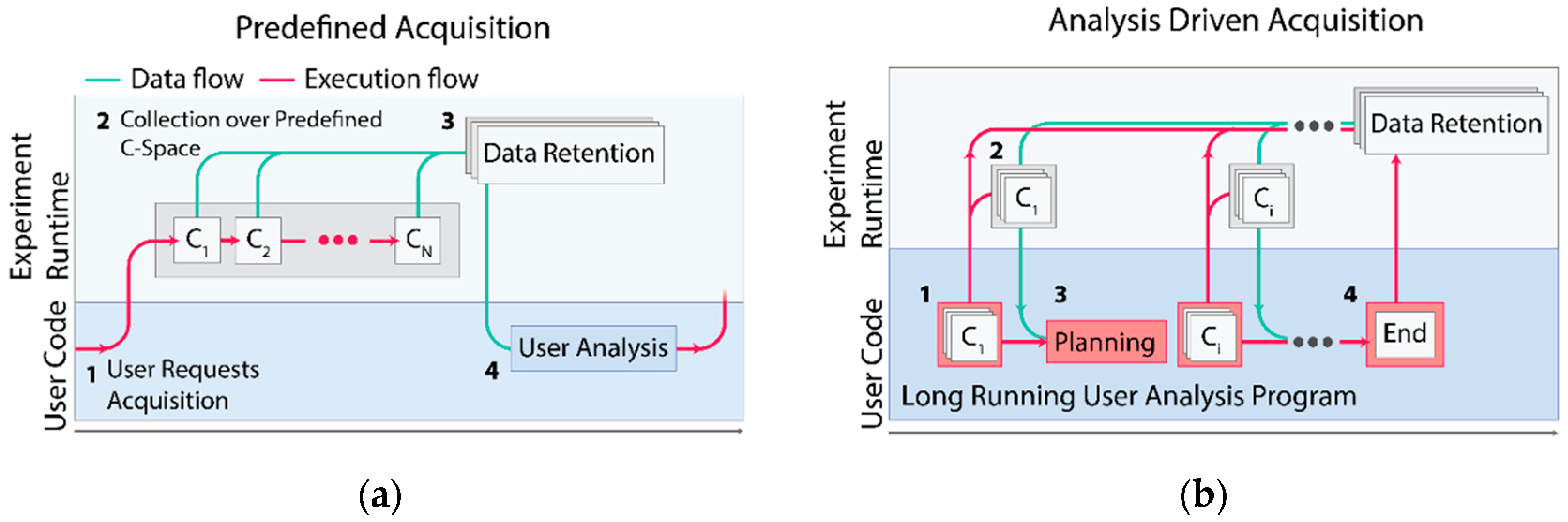
With this change, it becomes apparent to perform complex acquisitions under one of two different paradigms for data acquisition. Under the traditional paradigm, users can select a predefined acquisition program and issue collection over a predefined collection of experimental configurations (Figure 2a). Next, they can analyze their data before making further decisions about what data to collect. Alternatively, the fine-grained decisions about the next data point to collect can be made by a user analysis program running asynchronously on AutodiDAQt Receiver, as is shown in Figure 2b. The ability to perform acquisitions driven by analysis, or simply to rapidly adapt the acquisition in response to the experimental data, provides a leap in capability and experimental efficiency. Because data are available during acquisition, the experimenter is free to begin analysis and decision making using whatever tools they are most comfortable with.
It pays to be concrete, so here we will consider two examples that stem from photoemission spectroscopy. By considering nanoARPES and nanoXPS, where regions with distinct electronics and morphology require efficient use of acquisition time, we will explore two approaches that permit the rapid acquisition and interpretation of data. Using time-resolved ARPES (TARPES), we will see how the approach can improve the reliability and fidelity of recorded data and reconfigure the acquisition to defeat hardware limitations.

3.2. Application to NanoXPS
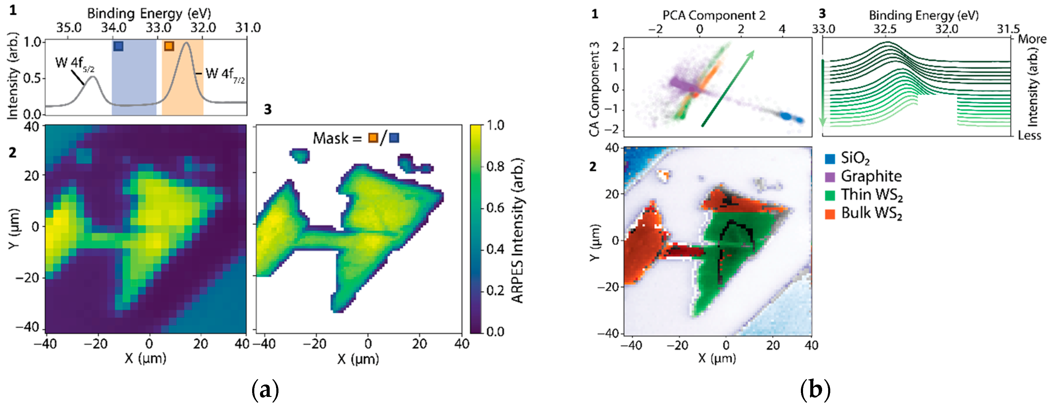
In Figure 3a(1–3), we show how even rudimentary applications of the analysis-in-the-loop would provide gigantic efficiency gains over data that were collected under standard acquisition controls. In Figure 3(a1), core-level spectra from a multilayer sample of WS2 were collected by coarsely rastering over a sample surface (Figure 3(a2)) using a nanoXPS setup. In the conducted experiment, which was performed with traditional DAQ software roughly following the scheme of Figure 2a, the resolution was increased by a factor of nine to resolve details in the sample morphology. However, analysis-in-the-loop, which adaptively increases the resolution only on a sample region with intense W 4f core levels (orange divided by blue regions in Figure 3(a1)), would have permitted acquiring data over only relevant portions of the sample, shown in Figure 3(a3), and would have used only 37% of the total acquisition time as was used in the measurement.
Other more sophisticated schemes, falling under the broader umbrella of machine-learning-in-the-loop, have been explored. One approach class based on Gaussian process (GP) regression has already demonstrated progress toward autonomous experimentation in photoemission spectroscopy [29]. Autonomous GP regression assumes, however, that all sources of variance in experimental data are salient, whereas most are not and can be rejected instantly by a domain expert. This contention between automation and domain expertise is likely to prevent the wide application of fully autonomous experimentation for a long time to come, with narrow exceptions for well-defined experimental tasks. Human-in-the-loop methods, which improve the decision-making power of scientists, are a more capable middle ground and promise to improve throughput while targeting the specific needs of scientists. Of course, these approaches can include machine learning, especially that used for exploratory data analysis. Figure 3b(1–3) illustrate an approach covering the same problem space as discussed in Figure 3a(1–3). Figure 3b1 shows a principal component analysis (PCA) decomposition of the XPS curves from the same sample region. Colored scatter cohorts are identified by visual clustering and correspond to sample morphology and content in Figure 3(b3). Although not principled in the sense of accurately modeling the experimental data’s distribution, rudimentary decompositions such as PCA rapidly provide insight that drives the efficient use of acquisition time. Decomposition features are also frequently highly correlated with relevant sample physics even if they provide no causal or generative information: in Figure 3(a3), it is apparent that PCA has identified a proxy for the inhomogeneous doping variations on the WS2 sample. In this scheme, machine learning is used for the rapid surveying and summarization of datasets, optimizing the use of available scientific expertise for decision making.

3.3. Application to Pump-Probe ARPES

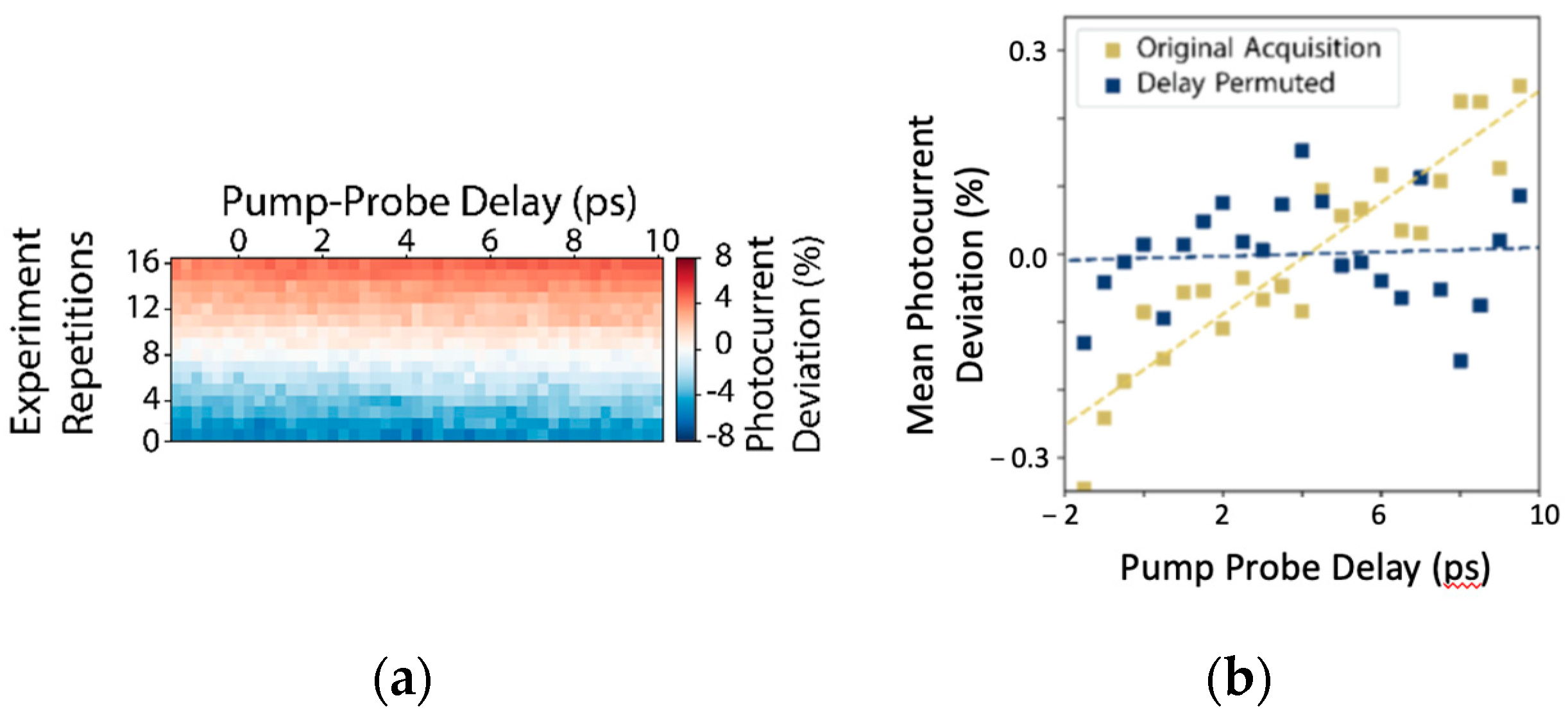
Alternatively, the analysis-in-the-loop approach provides scientists with the ability to rapidly adapt to changes in experimental conditions and to remove dataset bias, by treating software as a malleable tool rather than a fixed constraint. To give an example where this is valuable, we now turn to issues of systematic bias arising in pump-probe ARPES experiments. Because fourth harmonic or high harmonic generation is common in attaining DUV and XUV pulses from Ti:Sapph lasers, pump-probe ARPES experiments are especially susceptible to laser intensity fluctuations. These fluctuations can create confounding effects where infrared and UV doses can be highly correlated with measured delay time. These issues compound with other nonlinearities in the photoelectron detection process [44]. One very common way of minimizing this effect, if stabilizing the source power is not feasible, is to repeat the experiment in many short repetitions so that transients are better spread across different delays. Although not guaranteed to remove the correlation between delay and laser power, this approach is very common on photoemission apparatus because it is simple to shoehorn it into complicated data acquisition software merely by running additional sweeps. The resulting total dose delivered can be visualized in this scheme for an actual experiment in Figure 4a. Despite the appearance that this minimizes the effects of transients, when we average data across repetitions, we see that there is still a pernicious dependence of mean dose, measured by total photoelectron yield, as a function of the experimental delay, as in Figure 4b. Properly removing the bias requires stratifying individual experimental runs by dose cohort and randomly shuffling the acquisition order so that there can be no correlation. Adaptively accommodating these kinds of responses to issues arising during acquisition requires a dynamic and cooperative approach between acquisition and analysis. In this narrow case, AutodiDAQt provides support for acquisition shuffling in either of the supported acquisition paradigms.
In the broader context, deeper cooperation between DAQ-aware user analysis programs, such as PyARPES [9] in the context of angle-resolved photoemission spectroscopy, permit scientists to rapidly define acquisitions over trajectories that are challenging to define without expert knowledge. In this approach, it is straightforward to collect data along a particular path in a given material’s 2D surface Brillouin zone, or in the 3D bulk Brillouin zone.

4. Discussion

AutodiDAQt makes some assumptions about the data acquisition task to simplify the acquisition runtime. Significantly, because AutodiDAQt implements the acquisition runtime as a set of asynchronous tasks running on a single process, AutodiDAQt assumes that reads from instrumentation are IO bound rather than CPU bound. Although this is not a strict assumption, communication with another process that is set up during the application startup is still possible, circumventing this assumption requires that the end user take care of any multitasking concerns arising out of the partial adoption of multiprocessing.
Despite this constraint, the AutodiDAQt runtime is a very low overhead, as can be verified by running the profiling benchmarks included in the source repository. Benchmarks are always machine dependent, but on plain consumer hardware available at the time of publication, the overhead per experimental configuration (“point”) is in the order of 200   μ s when running an acquisition generating synthetic data from a 250 px by 250 px virtual CCD. As AutodiDAQt is not intended for applications that need to operate instruments in closed loop control or collect data in real-time, overheads of less than one millisecond per point makes the use of multiprocessing unnecessary for most experiments. AutodiDAQt achieves this level of performance by running UI repainting infrequently, using the Qt event loop in place of the standard library event loop, and by performing essentially no data bookkeeping other than memory allocation during an experimental run. All data collation and transformation is deferred to a separate process once an experiment is complete.

5. Conclusions

Compared to the existing approaches to the data acquisition task, AutodiDAQt represents a compromise between data acquisition simplicity and holism that makes it the ideal platform for scientists who do not want the writing of software to overshadow their central task: collecting and understanding data. By providing synchronous and isolated control and analysis via AutodiDAQt Receiver, this compromise is better seen as a strength, which we believe will enable a new generation of experiments driven by real-time ML analysis during the experiment. Analysis isolation encouraged by the remote broker design of AutodiDAQt minimizes the trust surface area between user code and DAQ code, making AutodiDAQt appropriate for experiments with many nonexpert users. As scientists are allowed to make more parsimonious use of time during experiment design and during acquisition, AutodiDAQt opens the door to treating data collection as a living and malleable part of the analysis process.

Supplementary Materials

The following supporting information can be downloaded at: https://www.mdpi.com/article/10.3390/software2010005/s1, A PDF file, including Figure S1: Products (top) and sums (bottom) of configuration spaces and programs; Figure S2: Code Listing; Figure S3: Generated UI and DAQ program for code listing 1; Figure S4: Output data for code listing 1; Figure S5: Structure of the AutodiDAQt Framework and Experiment Control Flow. References [45,46,47,48,49] are cited in the Supplementary Materials.

Author Contributions

Conceptualization, C.H.S. and A.L.; methodology, C.H.S.; software, C.H.S.; data curation, C.H.S.; writing—review and editing, C.H.S. and A.L.; visualization, C.H.S. and A.L.; supervision, A.L.; project administration, A.L.; funding acquisition, A.L. All authors have read and agreed to the published version of the manuscript.

Funding

This research was funded by the Director, Office of Basic Energy Sciences, Materials Science and Engineering Division, of the U.S. Department of Energy, under Contract No. DE-AC02-05CH11231, as part of the Ultrafast Materials Science Program (KC2203). The authors would like to thank Ping Ai and Jacob Gobbo for their assistance in the trial application AutodiDAQt to time-of-flight photoemission spectroscopy experiments and Daniel H. Eilbott for test application in terahertz spectroscopy experiments. The practical need for flexible acquisition software accompanying the development of these two new experiments in our lab were a proximate cause for developing AutodiDAQt from a software experiment into a usable system and their needs underpin the approach to data acquisition pursued here.

Institutional Review Board Statement

Not applicable.

Informed Consent Statement

Not applicable.

Data Availability Statement

The data that support the finding of this study are available from the corresponding author upon request.

Conflicts of Interest

The authors declare no conflict of interest.

References

  1. Celestre, R.; Nowrouzi, K.; Shapiro, D.A.; Denes, P.; Joseph, P.M.; Schmid, A.; Padmore, H.A. Nanosurveyor 2: A compact instrument for nano-tomography at the advanced light source. J. Phys. Conf. Ser. 2017, 849, 012047. [Google Scholar] [CrossRef] [Green Version]
  2. Cheng, Y. Single particle cryo-EM-How did it get here and where will it go. Science 2018, 361, 876. [Google Scholar] [CrossRef] [Green Version]
  3. Egelman, E.H. The current revolution in cryo-EM. Biophys. J. 2016, 110, 1008. [Google Scholar] [CrossRef] [Green Version]
  4. Schermelleh, L.; Ferrand, A.; Huser, T.; Eggeling, C.; Sauer, M.; Biehlmaier, O.; Drummen, G.P.C. Super-resolution microscopy demystified. Nat. Cell Biol 2019, 21, 72. [Google Scholar] [CrossRef]
  5. Zipfel, W.R.; Williams, R.M.; Webb, W.W. Nonlinera magic: Multiphoton microscopy in the bioscience. Nat. Biotechnol. 2003, 21, 1369. [Google Scholar] [CrossRef]
  6. Wang, H.; Rivenson, Y.; Jin, Y.; Wei, Z.; Gao, R.; Günaydın, H.; Bentolila, L.A.; Kural, C.; Ozcan, A. Deep learning enables cross-modality super-resolution in fluorescence microscopy. Nat. Methods 2019, 16, 103. [Google Scholar] [CrossRef]
  7. Damascelli, A.; Hussain, Z.; Shen, Z.X. Angle resolved photoemission studies of the cuprate superconductors. Rev. Mod. Phys. 2003, 75, 473. [Google Scholar] [CrossRef] [Green Version]
  8. Lin, C.Y.; Moreschini, L.; Lanzara, A. Present and future trends in spin ARPES. Europhys. Lett. 2021, 134, 57001. [Google Scholar] [CrossRef]
  9. Stansbury, C.; Lanzara, A. PyARPES: An analysis framework for multimodal angle resolved photoemission spectroscopies. SoftwareX 2020, 11, 100472. [Google Scholar] [CrossRef]
  10. Day, R.P.; Zwartsenberg, B.; Elfimov, I.S.; Damascelli, A. Computational framework chinook for angle-resolved photoemission spectroscopy. NPJ Quantum Mater. 2019, 4, 1. [Google Scholar] [CrossRef] [Green Version]
  11. Kim, Y.; Oh, D.; Huh, S.; Song, D.; Jeong, S.; Kwon, J.; Kim, M.; Kim, D.; Ryu, H.; Jung, J.; et al. Deep learning-based statistical noise reduction for multidimensional spectral data. Rev. Sci. Instrum. 2021, 92, 073901. [Google Scholar] [CrossRef]
  12. Peng, H.; Gao, X.; He, Y.; Li, Y.; Ji, Y.; Liu, C.; Ekahana, S.A.; Pei, D.; Liu, Z.; Shen, Z.; et al. Super resolution convolutional neural network for feature extraction inn spectroscopic data. Rev. Sci. Instrum. 2020, 91, 033905. [Google Scholar] [CrossRef]
  13. He, Y.; Wang, Y.; Shen, Z.-X. Visualizing dispersive features in 2D image via minimum gradient method. Rev. Sci. Instrum. 2017, 88, 073903. [Google Scholar] [CrossRef] [Green Version]
  14. Avila, J.; Asensio, M.C. First NaanoARPES User Facility Available at SOLEIL: An Innovative and Powerful Tool for Studying Advanced Materials. Synchrotron Radiat News 2014, 27, 24. [Google Scholar]
  15. Bostwick, A.; Rotenberg, E.; Avila, J.; Asensio, M.C. Zooming in electronic structure: NanoARPES at SOLEIL and ALS. Synchrotron Radiat. News 2012, 25, 19. [Google Scholar] [CrossRef]
  16. Rotenberg, E.; Bostwick, A. MicroARPES and nanoARPES at diffraction-limited light sources: Opporttuniities and performance gains. J. Synchrotron Radiat. 2014, 21, 1048. [Google Scholar] [CrossRef]
  17. Jozwiak, C.; Graf, J.; Lebedev, G.; Andresen, N.; Schmid, A.K.; Fedorov, A.V.; Gabaly, F.E.; Wan, W.; Lanzara, A.; Hussain, Z. A high efficiency spin-reesolved photoemission nspectrometer combining time-of-flight spectroscopy with exchange-scattering polarimetry. Rev. Sci. Instrum. 2010, 81, 053904. [Google Scholar] [CrossRef] [Green Version]
  18. Medjanik, K.; Fedchenko, O.; Chernov, S.; Kutnyakhov, D.; Ellguth, M.; Oelsner, A.; Schönhense, B.; Peixoto, T.R.F.; Lutz, P.; Min, C.-H.; et al. Direct 3D mapping of the Fermi surface and Fermi velocity. Nat. Mater. 2017, 16, 615–621. [Google Scholar] [CrossRef]
  19. Kutnyakhov, D.; Xian, R.P.; Dendzik, M.; Heber, M.; Pressacco, F.; Agustsson, S.Y.; Wenthaus, L.; Meyer, H.; Gieschen, S.; Mercurio, G.; et al. Time and momentum resolved photoemission studies using time of flight momentum microscopy at a free-electron laser. Rev. Sci. Instrum. 2020, 91, 013109. [Google Scholar] [CrossRef]
  20. Kastl, C.; Chen, C.T.; Koch, R.J.; Schuler, B.; Kuykendall, T.R.; Bostwick, A.; Jozwiak, C.; Seyller, T.; Rotenberg, E.; Weber-Bargioni, A.; et al. Multimodal spectromicroscopy of monolayer WS2 enabled by ultra-clean van der Waals epitaxy. 2D Mater. 2018, 5, 045010. [Google Scholar] [CrossRef]
  21. Wilson, N.R.; Nguyen, P.V.; Seyler, K.; Rivera, P.; Marsden, A.J.; Laker, Z.P.L.; Constantinescu, G.C.; Kandyba, V.; Barinov, A.; Hine, N.D.M.; et al. Determination of band offsets, hybridization and exciton binding in 2D semiconductor heterostructures. Sci. Adv. 2017, 3, e1601832. [Google Scholar] [CrossRef] [Green Version]
  22. Stansbury, C.H.; Utama, M.I.B.; Fatuzzo, C.G.; Regan, E.C.; Wang, D.; Xiang, Z.; Ding, M.; Watanabe, K.; Taniguchi, T.; Blei, M.; et al. Visualizing electron localization of WS2/WSe2 moire’ superlattices in momentum space. Sci. Adv. 2021, 7, eabf4387. [Google Scholar] [CrossRef]
  23. Utama, M.I.B.; Koch, R.J.; Lee, K.; Leconte, N.; Li, H.; Zhao, S.; Jiang, L.; Zhu, J.; Watanabe, K.; Taniguchi, T.; et al. Visualizaation of the flaat electronic band in twisted bilayer graphene near the magic angle twist. Nat. Phys. 2020, 1, 184–188. [Google Scholar]
  24. Lisi, S.; Lu, X.; Benschop, T.; de Jong, T.A.; Stepanov, P.; Duran, J.R.; Margot, F.; Cucchi, I.; Cappelli, E.; Hunter, A.; et al. Observation of flat bands in twisted bilayer graphene. Nat. Phys. 2021, 17, 189. [Google Scholar] [CrossRef]
  25. Ulstrup, S.; Koch, R.J.; Singh, S.; McCreary, K.M.; Jonker, B.T.; Robinson, J.T.; Jozwiak, C.; Rotenberg, E.; Bostwick, A.; Katoch, J.; et al. Direct observation of minibands in a twisted graphene/WS2 bilayer. Sci. Adv. 2020, 6, eaay6104. [Google Scholar] [CrossRef] [Green Version]
  26. Nguyen, P.V.; Teutsch, N.C.; Wilson, N.P.; Kahn, J.; Xia, X.; Graham, A.J.; Kandyba, V.; Giampietri, A.; Barinov, A.; Constantinescu, G.C.; et al. Visualizing electrostatic gating effects in two dimensional heterostructures. Nature 2019, 572, 220–222. [Google Scholar] [CrossRef] [Green Version]
  27. Joucken, F.; Avila, J.; Ge, Z.; Quezada-Lopez, V.; Yi, H.; Le Goff, R.; Baudin, E.; Davenport, J.L.; Watanabe, K.; Taniguchi, T.; et al. Visualizing the Effect of an electrostatic gate with angle resolved photoemission spectroscopy. Nano Lett. 2019, 19, 2682. [Google Scholar] [CrossRef] [Green Version]
  28. Jones, A.J.H.; Muzzio, R.; Majchrzak, P.; Pakdel, S.; Curcio, D.; Volckaert, K.; Biswas, D.; Gobbo, J.; Singh, S.; Robinson, J.T.; et al. Observation of electrically tunable van hove singularities in twisted bilayer graphene from nanoARPES. Adv. Mater. 2020, 32, 2001656. [Google Scholar] [CrossRef]
  29. Melton, C.N.; Noack, M.M.; Ohta, T.; Beechem, T.E.; Robinson, J.; Zhang, X.; Bostwick, A.; Jozwiak, C.; Koch, R.J.; Zwart, P.H.; et al. K-means-driven Gaussian process data collection for angle resolved photoemission spectroscopy. Mach. Learn. Sci. Technol. 2020, 1, 045015. [Google Scholar] [CrossRef]
  30. Noack, M.M.; Yager, K.G.; Fukuto, M.; Doerk, G.S.; Li, R.; Sethian, J.A. A Kriging-based approach to autonomous experimentation with applications to x-ray scattering. Sci. Rep. 2019, 9, 11809. [Google Scholar] [CrossRef] [Green Version]
  31. Flores-Leonar, M.M.; Mejía-Mendoza, L.M.; Aguilar-Granda, A.; Sanchez-Lengeling, B.; Tribukait, H.; Amador-Bedolla, C.; Aspuru-Guzik, A. Materials Acceleration platforms: On the way to autonomous experimentation. Curr. Opin. Green Sustain. Chem. 2020, 25, 100370. [Google Scholar] [CrossRef]
  32. Castle, J.E.; Baker, M.A. The feasibility of an XPS expert system demonstrated by a rule set for carbon contamination. J. Electron Spectrosc. Relat. Phenom. 1999, 105, 245–256. [Google Scholar] [CrossRef]
  33. Zahl, P.; Bierkandt, M.; Schröder, S.; Klust, A. The flexible and modern open source scanning probe microscopy software package GXSM. Rev. Sci. Instrum. 2003, 74, 1222. [Google Scholar] [CrossRef]
  34. Horcas, I.; Fernández, R.; Gómez-Rodríguez, J.M.; Colchero, J.; Gómez-Herrero, J.; Baro, A.M. WSXM: A software for scanning probe microscopy and a tool for nanotechnology. Rev. Sci. Instrum. 2007, 78, 013705. [Google Scholar] [CrossRef] [Green Version]
  35. Jermain, C.; Minhhai; Rowlands, G.; Girard, H.-L.; Schippers, C.; Schneider, M.; Chweiser; Buchner, C.; Spirito, D.; Feinstein, B.; et al. Ralph-Group/Pymeasure: PyMeasure 0.8; Zenodo; Organisation Europenne Pour la Recherche Nucleaire: Geneva, Switzerland, 2020. [Google Scholar]
  36. Bogdanowicz, N.; Rogers, C.; Zakv; Wheeler, J.; Pelissier, S.; Marazzi, F.; Eedm; Galinskiy, I.; Abril, N. Mabuchilab/Instrumental: 0.6; Zenodo; Organisation Europenne Pour la Recherche Nucleaire: Geneva, Switzerland, 2020. [Google Scholar]
  37. Koerner, L. Instrbuilder: A python package for electrical instrument control. J. Open Source Softw. 2019, 4, 1172. [Google Scholar] [CrossRef]
  38. Rowlands, G.; Ribeill, G.; Ryan, C.; Ware, M.; Johnson, B.; Kalfus, B.; Fallek, S.; Hai, M.; Mcgurrin, R.; Ellard, D.; et al. Auspex. 2021. Available online: https://github.com/BBN-Q/Auspex (accessed on 21 January 2020).
  39. Weber, S.J. PyMoDAQ: An open-source python-based software for modular data acquisition. Rev. Sci. Instrum. 2021, 92, 045104. [Google Scholar] [CrossRef]
  40. The Lanzara Group. Available online: https://github.com/chstan/arpes (accessed on 16 January 2023).
  41. Koerner, L.J.; Caswell, T.A.; Allan, D.B.; Campbell, S.I. A python data control and acquisition suite for reproducible research. IEEE Trans. Instrum. Meas. 2020, 69, 1698. [Google Scholar] [CrossRef]
  42. The LabRAD Authors, LabRAD (n.d.). Available online: https://github.com/labrad/pylabrad (accessed on 16 January 2023).
  43. The Bluesky Authors, Bluesky. 2021. Available online: https://blueskyproject.io (accessed on 16 January 2023).
  44. Reber, T.J.; Plumb, N.C.; Waugh, J.A.; Dessau, D.S. Effects, determination and correction of count rate nonlinearity in multi-channel analog electron detectors. Rev. Sci. Instrum. 2014, 85, 043907. [Google Scholar] [CrossRef] [Green Version]
  45. van der Walt, S.; Colbert, S.C.; Varoquaux, G. The NumPy array: A structure for efficient numerical computation. Comput. Sci. Eng. 2011, 13, 22. [Google Scholar] [CrossRef] [Green Version]
  46. Virtanen, P.; Gommers, R.; Oliphant, T.E.; Haberland, M.; Reddy, T.; Cournapeau, D.; Burovski, E.; Peterson, P.; Weckesser, W.; Bright, J.J.; et al. SciPy1.0: Fundamental algorithms for scientific computing in Python. Nat. Methods 2020, 17, 261. [Google Scholar] [CrossRef] [Green Version]
  47. Hamman, J.; Hoyer, S. Xarray: N-D labeled arrays and datasets in Python. J. Open Res. Softw. 2017, 5, 10. [Google Scholar]
  48. Wes McKinney, W. Pyton for Data Analysis; O’Reilly Media Inc.: Sebastapol, CA, USA, 2011. [Google Scholar]
  49. Miles, A.; Kirkham, J.; Durant, M.; Bourbeau, J.; Onalan, T.; Hamman, J.; Patel, Z.; Shikharsg; Rocklin, M.; Dussin, R.; et al. Zarr-Developers/Zarr-Python: V2.4.0; Zenodo; Organisation Europenne Pour la Recherche Nucleaire: Geneva, Switzerland, 2020. [Google Scholar]
Figure 1. User interface generation. ((a), 1–4) Elements of the default user interface provided by AutodiDAQt and their correspondence to data acquisition hardware. (a1) Acquisition hardware and software drivers express degrees of freedom (axes) and capabilities (settings, functions) for instruments. (a2) Hardware capabilities are mapped to a uniform representation for experimental degrees of freedom and experimental states in AutodiDAQt. In certain contexts, this mapping can be built automatically by driver introspection. Otherwise, an expressive API for defining the hardware semantics of an experiment is available. Device semantics cover details of how to invoke instrument methods to control hardware, limits on values, their concrete types, and their role in an experiment. (a3) User interface elements corresponding to each degree of freedom and capability of the hardware are provided automatically and synchronize automatically with the data acquisition program state. (a4) Degrees of freedom defined in the software representation of (a2) can be automatically composited into acquisition programs, with associated software generated controls. The complex user interface programming tasks of (a3,a4), in fact most data acquisition software and interfaces, can be handled automatically by adopting a uniform software representation for the degrees of freedom of the hardware. The leftmost panel shows the main acquisition window with acquisition status, data streams, acquisition program queue, and acquisition parameters. (b) At a more fine-grained level, users can use the UI generation primitives for basic types, composite data structures, and classes. In the cases where acquisitions are parameterized—for instance, by the range over which to acquire data, the number of points to collect, or the details of control flow such as logging details or whether to wait after motion—AutodiDAQt will generate appropriate controls for the parameters that will be used at the beginning of an acquisition. If the user assigns multiple independent modes of collecting data, a control for the active collection mode will be generated as well.
Software 02 00005 g001
Figure 2. Analysis-driven acquisition. ((a), 1–4) (a,b) Supported data collection paradigms. (a) In traditional conceptions of data acquisition, a scientist selects from a limited menu of predefined collection modes over a fixed coordinate space. Once requested (1a), the system collects data over the states C i (2a) of this space until all data are available, at which point the system retains the data for later analysis (3a). The scientist inspects the data (4a) and the process is repeated. (b) Analysis-in-the-loop conception of data acquisition. A scientist submits a program to the acquisition system (1b). The program can issue acquisition instructions that are validated and performed by the acquisition system (2b) and intermediate data are collected as well as provided back to the program. In response to the acquired data or as part of a pre-existing acquisition strategy, the scientist’s program can issue additional instructions (3b), which are iteratively handled until the program decides the acquisition is finished (4b).
Software 02 00005 g002
Figure 3. nanoARPES Opportunities for Analysis-Driven Acquisition. (a1) Tungsten 4f core-level X-ray photoelectron spectrum at a specific location (a2) Tungsten 4f core-level X-ray photoelectron spectrum as a function of position (a3) Tungsten 4f core-level X-ray photoelectron spectrum at binding energy shown in the blue and orange areas of (a1). (b1) Coarse nanoXPS image providing sample topography, with complex region-of-interest. (b2) High-resolution experiment trajectory on sample regions with intense W 4f peak (blue divided by orange energy region). Collected area occupies 37% of total scan window. (b1b3) Integrating machine learning into the analysis–acquisition loop permits rapid understanding of the sample morphology and efficient use of acquisition time. (b1) PCA component projection for XPS curves across the sample surface colored according to their composition (labels at right of (b3)). (b2) Spatial map of all XPS curves across the sample corresponding to scattered points in (b2) showing correspondence to distinct physical regions on the sample. (b3) W 4 f 7 / 2 level green WS2 multilayer region of the sample corresponding to spatial cohorts with varying PCA components (green arrow in (b2)). Even coarse decompositions such as PCA map onto physically interpretable qualities such as inhomogeneous doping across the sample surface inducing shifts in the peak locations seen by nanoXPS.
Software 02 00005 g003
Figure 4. Using analysis-in-the-loop to improve experimental reliability. (a,b) Scan primitives provide options to reduce systematic bias in time-resolved angle-resolved photoemission spectroscopy experiments. (a) laser power fluctuations over a Tr-ARPES experiment acquired by traversing delay and repetitions in major delay order. (b) Systematic bias due to small laser power variations throughout the experiment (yellow dots and trend), which are removed by acquiring data in random order (simulated with identical variability, blue points).
Software 02 00005 g004
Disclaimer/Publisher’s Note: The statements, opinions and data contained in all publications are solely those of the individual author(s) and contributor(s) and not of MDPI and/or the editor(s). MDPI and/or the editor(s) disclaim responsibility for any injury to people or property resulting from any ideas, methods, instructions or products referred to in the content.

