Market Crashes and Time-Translation Invariance

Abstract

The general framework for quantitative technical analysis of market prices is revisited and extended. The concept of a global time-translation invariance and its spontaneous violation and restoration is introduced and discussed. We find that different temporal patterns leading to some famous crashes (e.g., bubbles, hockey sticks, etc.) exhibit analogous probabilistic distributions found only in the time series for the stock market indices. A number of examples of crashes are presented. We stress that our goal here is to study the crash as a particular phenomenon created by spontaneous time-translation symmetry breaking/restoration. We ask only “how to calculate and interpret the probabilistic pattern which we encounter in the day preceding crash, and how to calculate the typical market reactions to shock?”.

1. Introduction

The famous physicist Frederic Joliot-Curie pioneered a fundamental symmetry approach to natural sciences. He stated that, for the occurrence of a phenomenon, some original and relevant property of symmetry must be broken. Spontaneous symmetry breaking happens without the presence of any asymmetric cause [1].

Modern financial theory is geared towards ergodicity violations. Ergodicity violations [2,3,4,5] may be understood as a manifestation of a violation of the time invariance of a random process. One can think that seasonality effects in a time series could represent its classical analog of a spontaneous breaking of time-translation symmetry in quantum systems [6].

The concept of spontaneously broken time-translation invariance can be useful in application to market dynamics [7]. The relative probabilities of the evolution patterns could be derived from the stability considerations. The probability introduced in [8] is closer to the time probability, concerned with a single person living through time, see [4,5].

Assume that numerical data on the price s are available in the given time domain. I.e., there is a known sequence of $N+1$ values

$$s\left(t_0\right),s\left(t_1\right),\dots ,s\left(t_N\right),$$

for corresponding $N+1$ equidistant successive moments in time $t=t_j$, where $j=0,1,2\dots ,N.$ In finance, one is interested primarily in the value of log-return (see, e.g., [9]).

$$R(t_N+\delta t)=ln\left(\frac{s(t_N+\delta t)}{s\left(t_N\right)}\right).$$

(1)

Mind that a catastrophic downward acceleration regime (for the prices) is known as a crash [10]. Market price dynamics in the vicinity of a crisis (crash, melt-up) could be treated as a self-similar evolution, because of the prevalence of the collective crowd behavior [8,11,12]. Prediction markets [13] often work pretty well; however, there are many cases when they give wrong predictions or make any prediction at all. It could be reasonably speculated that market crowds can have collective breakdowns and tend to wrongly assess the risks of the stock market crashes [14].

We intend to develop some consistent technique for spontaneous symmetry breaking with its subsequent restoration, thus extending further the ideas and methods of [7].

2. Self-Similarity and Time-Translation Invariance

The proper laws of nature are supposed to respect self-similarity. In particular, in classical mechanics they are formulated in a form that respects a time-translation invariance [15].

One would like to find and formulate mathematically the corresponding underlying symmetry for price dynamics. Really, during the times perceived as normal one can expect an approximate price growth rate or a constant return. The average price trajectory is expected to be exponential and reflect the power of compounding interests. Then, as explained in [5], the so-called expected forward price is given by the exponential function.

$$F_t^P=s_{t_0}exp\left(\beta (t-t_0)\right).$$

(2)

Here, $s_{t_0}$ is an underlying index or security price at $t=t_0$, and $F_t^P$ stands for the fair value of the future requiring a risk associated with expected return $\beta$.

The financial markets tend to deviate from such simple descriptions. The bubbles are formed, as well as various temporal patterns considered by technical analysis. However, the fundamental value is not directly observable, greatly complicating the urgent practical task of defining time intervals where such deviations persist. The causes of deviation were explained in [10,16].

Let us accept a self-similar evolution for the marker price s. More precisely, one can see that

$$s(t+\tau ,a)=s(t,s(\tau ,a\left)\right),$$

(3)

for an arbitrary shift $\tau$. The corresponding initial condition

$$s(0,a)=a,$$

(4)

is valid [17,18,19].

The linear function (regression) obviously satisfies the desired property (3), as expalained in great detail in [20,21]. The polynomial regression obtained in a standard way serves as the expansion of the price to be improved by applying some resummation procedure expressed by the exponential and super-exponential approximants [7].

Let us obtain the linear regression on the data around the origin $t_0=0$,

$$s_{0,1}\left(t\right)=a_1+b_{1}t.$$

The point of origin is arbitrary and can be moved to an arbitrary position (origin) specified by the real number r, so that

$$s_{r,1}\left(t\right)=A_1\left(r\right)+B_1\left(r\right)(t-r).$$

(5)

The coefficients are related, i.e.,

$$A_1\left(r\right)=a_1+b_{1}r,B_1\left(r\right)=b_1,$$

and

$$s_{r,1}\left(t\right)\equiv s_{0,1}\left(t\right).$$

Each of the replicas $s_{r,1}\left(t\right)$ respects the time-translation symmetry, which can be called then a global time invariance. When one considers the linear “approximant” (5) for extrapolation, the prediction for the same moment of the future will not depend on r.

Eventually, we will have to find the position of origin r explicitly, from some resummation and optimization procedures. The resummation procedure will have to break the replica symmetry, while optimization will have to restore the symmetry. Most importantly, the form (5) can be used constructively, as discussed below.

Exponential function also satisfies conditions (3) and (4), as elaborated in the paper [20]. The exponential function can be replicated as explained in [20]. The replicas $E_r\left(t\right)$ are time-translation invariant. Again, the prediction by the $E_r\left(t\right)$ for the same moment of the future will not depend on r [20]. In addition, each of the replicas still respects the time-translation symmetry, which can be considered as a global time invariance. More examples of self-similar functions can be found in the papers [20,22].

Obviously, if the exponential is obtained by fitting data, the fit will possess the global time-translation symmetry as well as the replica symmetry.

In order to break the symmetries, one should proceed differently. The polynomial regression can be transformed to the sought exponential form by means of the exponential approximants [7]. However, when the exponential approximant $E_1^{*}(t,r)$ is derived as asymptotically equivalent, say to the linear regression represented in form (5), we arrive to the form

$$E_1^{*}(t,r)=A_1\left(r\right)exp\left(\frac{B_1\left(r\right)}{A_1\left(r\right)}\left(t-r\right)\right),$$

(6)

with r-dependent ratio $\frac{B_1\left(r\right)}{A_1\left(r\right)}\equiv \beta \left(r\right)$. Thus, the replica symmetry is broken, when one considers the approximant (6) for extrapolation, meaning that the prediction for the same moment of the future will depend on origin r. Having $\beta$ dependent on r (and (or) t) in Formula (6) violates replica symmetry. As a consequence, instead of a global time-invariant law of motion, producing extrapolations in time independent of r, we have a set of local laws near each point of origin r.

Yet, each of the replicas still respects the time-translation symmetry. Instead of the global properties expressed in relations (3) and (4), we have a local time invariance symmetry. Then, which one of the local laws is correct, and how can it be selected?

We suggest below some relatively simple techniques for finding local laws and finding an optimal one in the following subsections. However, having r in such a formula fixed by imposing some additional, optimal condition, will completely (or partially) restore the globally symmetric law of motion.

Some other symmetries, such as shape invariance [23], scaling invariance [24] and discrete scale invariance [16], are discussed in more detail in the companion paper [20]. Gauge symmetry is also known and could be employed in finance [25].

In the companion paper [20], we discuss some techniques that account for higher-order terms in regression, making $\beta$ also a time-dependent $\beta (r,t)$. Instead of a single relaxation time we can have an effective relaxation time, as expounded extensively in [20]. In our study, $\beta$ plays the same role as the expected growth rate of multiplicative random processes and could be optimized directly, in principle [2,4].

2.1. Higher-Order Regression, Approximants and Multipliers

In the current paper, we intend to extend the quantitative technical analysis of the paper [7], by employing the higher-degree regressions. Yet, our primary goal is to advance some consistent technique for the global time invariance and replica symmetry breaking, with their subsequent restoration.

The higher-order regressions adhere to the replica symmetry as well. The quadratic regression

$$s_{0,2}\left(t\right)=a_2+b_{2}t+c_2{t}^2,$$

can be replicated as follows:

$$s_{r,2}\left(t\right)=A_2\left(r\right)+B_2\left(r\right)(t-r)+C_2\left(r\right){(t-r)}^2,$$

with

$$A_2\left(r\right)=a_2+b_{2}r+c_2{r}^2,B_2\left(r\right)=b_2+2c_{2}r,C_2\left(r\right)=c_2,$$

so that

$$s_{r,2}\left(t\right)\equiv s_{0,2}\left(t\right),$$

(7)

i.e., the quadratic regression respects the replica symmetry. Explicit formulas for the fourth-order regressions can be found in the companion papers [20,21].

For the second-order regression, we have for practical purposes of extrapolation the concrete approximation

$$E_1^{*}(t,r)=A_2\left(r\right)exp\left(\frac{B_2\left(r\right)}{A_2\left(r\right)}\left(t-r\right)\right),$$

(8)

which is analogous to Formula (6). Of course, everything stated above on replica symmetry and its violation/restoration for approximant (6) holds for approximant (8) and look-alike approximations, to be employed in an arbitrary order of basic regression.

When extrapolations are accomplished by means of the $E_1^{*}(t_N+\delta t,r)$, they turn out to be different for various r. The latter means a breaking of the replica symmetry. Of course, the global time-translation symmetry is broken as well. Moreover, when we advance from the polynomial regressions to the exponential approximations, we are confronted with the whole emergent spectrum of relaxation (growth) times [20,21]. The spectrum could be continuous or discrete. The methods of finding the spectrum will be discussed further on.

For approximants (6) and (8), we can introduce the so-called multipliers [8,20]

$$M_1^{*}(t,r)=exp\left(\frac{B\left(r\right)}{A\left(r\right)}(t-r)\right),$$

(9)

explicitly and in a simple form. Multipliers characterize the stability of the approximants. Simple exponential approximations allow, among other things, a nice graphical representation of the probabilities expressed as the relation (10), as shown below.

Now, one can introduce introduce probability for each solution [8,20]

$$Probability\propto {\left|M_1^{*}(t,r)\right|}^{-1},$$

(10)

with proper normalization [8].

By analogy, one can also construct for the quadratic regression and alikes the second-order super-exponential approximant [26],

$$E_2^{*}(t,r)=A_4\left(r\right)exp\left(\frac{B_2\left(r\right)}{A_2\left(r\right)}(t-r)exp\left(T_2\left(r\right)\frac{C_2\left(r\right)}{B_2\left(r\right)}(t-r)\right)\right),$$

(11)

with the control function $T_2\left(r\right)=1-\frac{B_2{\left(r\right)}^2}{2A_2\left(r\right)C_2\left(r\right)}.$ The first- and second-order approximants can be trivially extended to the higher order.

2.2. Methods of Finding Origin

We recognize here three main approaches to constructing approximants.

The first approach is the most conventional. It amounts to an improvement in the quality of the approximations by adding new information at each approximation step. At every step, the approximants are getting even more complex [27].

The second approach prescribes the correct form of the solution already in the starting approximation. The starting zero approximation is corrected then by asymptotically matching the corrected approximations with the truncated series/regressions [27].

The third approach emerges when the form and order of the approximants are kept the same in all orders. However, the underlying regressions are let to evolve into higher orders. In all orders of regression, we employ the very same form given by the exponential approximants, but with parameters changing numerically in different orders. In the current paper, we are mostly dealing with the third approach.

The position of origin is considered as an optimization parameter. To such an end, the following procedures are recommended. They include a continuous and a discrete spectrum of the origins.

1. The origin is to be considered as a dummy variable and will be integrated out, as first suggested in the companion paper [20]. The formula

$$I(t,T)=\frac{{\int }_{t_0-T}^{{}^{t_N+T}}{E}_1^{*}(X,t){\left|M_1^{*}(X,t)\right|}^{-1}dX}{{\int }_{t_0-T}^{{}^{t_N+T}}{\left|M_1^{*}(X,t)\right|}^{-1}dX},$$

(12)

is brought here for a completeness of presentation, while more discussion can be found in the paper [20]. The result of integration is required to satisfy the condition

$$I(t_N,T)=s\left(t_N\right).$$

(13)

From Equation (13), one has to find the integration limit $T=T{}^{*}$.

2. The additional condition of the same type is to be imposed directly on the exponential predictors without previous integration. i.e.,

$$E_1^{*}(t_N,r)=s\left(t_N\right).$$

(14)

One has to solve Equation (14) in order to define the particular few isolated origin(s) $r=r^{*}$ and arrive at a discrete spectrum of origins [20]. In the discrete spectrum consisting of M solutions, one can also apply the averaging procedure [20], leading to the predictor ${\overline{E}}_1$ given by Equation (48), from the companion paper [20]. It can be understood as a discrete version of Formula (12) for the continuous spectrum. With only the most stable solution selected for extrapolation we have the time-translation invariance restored completely. But when the average ${\overline{E}}_1$ is considered the symmetry is restored only partially.

Some of the solutions in the discrete spectrum do follow the raw data rather closely. Such a situation could be considered as “normal”. Such solutions tend to be less stable, with multipliers ∼1.

Otherwise, the solutions adhering to the data rather loosely are considered as “anomalous”. They are formally the most stable with small multipliers. Anomalous solutions are of paramount importance for our study. They correspond to crashes (melt-downs) and to the opposite of the crash situation, a melt-up. The discrete spectrum of scenarios is shown in Figure 1. The case of melt-ups should be studied separately.

Different approximants can be replicated and corresponding calculations involving the discrete spectrum can be performed as well. By analogy, one can construct the second-order super-exponential approximant (11), with the following equation on origins

$$E_2^{*}(r,t_N)=s\left(t_N\right),$$

(15)

to be solved.

The second method of optimization seems to be the most adequate and practical. It will be employed the most.

2.3. Ad Hoc Approximants

The third approach to constructing approximants can be developed further to also include explicitly the second-order terms from the regression. In addition to the exponential approximants, one can produce higher-order approximants, which would respect the time-translation symmetry. Such approximants are presented below and are discussed in great detail in the companion paper [20].

They could be viewed as ad hoc approximants. The idea is to create a closed-form approximation that can be realized only in special situations within low-order regressions. In contrast, the super-exponential approximants could be easily extended into the higher orders [26]. In fact, there is no formal limitation on the order of regression if such approximants are employed.

However, all approximants mentioned for the first approach to creating approximants systematically [27] do tend to violate the time-translation symmetry. Thus, they can not be used for the purposes of a complete replica symmetry and global time-translation symmetry restoration. That is why we are particularly interested in developing such ad hoc, special forms/approximants with an explicit preservation of the property of a time-translation invariance.

The motivation and reasoning behind the introduction of the logistic approximants is explained in the papers [20,21]. The so-called logistic function is time-translation invariant. The logistic approximant, in its general, r-dependent form, is designed to violate both replica symmetry and global time-translation invariance but becomes replica-invariant and respects global time invariance when the origin is fixed by an optimization of the type discussed in the preceding Section 2.2, with the exponential approximant to be simply replaced by the logistic approximant.

The logistic approximant was suggested in the following form,

$$L(t,r)=\frac{1}{q_2\left(r\right)+\frac{(1-q_1\left(r\right)q_2\left(r\right))exp(-q_0\left(r\right)(t-r))}{q_1\left(r\right)}},$$

with the corresponding multiplier

$$M_L(t,r)=\frac{q_0\left(r\right)e^{q_0\left(r\right)(-(t-r))}(1-q_1\left(r\right)q_2\left(r\right))}{B\left(r\right)q_1\left(r\right){\left(\frac{e^{q_0\left(r\right)(-(t-r))}(1-q_1\left(r\right)q_2\left(r\right))}{q_1\left(r\right)}+q_2\left(r\right)\right)}^2}.$$

All the parameters in the formulas above can be found explicitly and are presented in the companion paper [21]. The parameter r has to be found from the optimization of the type discussed in the preceding Section 2.2.

Another approximation can be developed from the Gompertz function [28]. The motivation and reasoning behind the introduction of the Gompertz approximants is explained in the paper [20]. The Gompertz approximant could be developed from the Gompertz function and underlying regression formulas, i.e.,

$$G(t,r)=g_0\left(r\right)exp(g_1\left(r\right)exp\left(g_2\left(r\right)(t-r)\right)),$$

with the corresponding multiplier $M_G(t,r)$ defined in [20]. Again, all the parameters can be found in explicit form and are presented in the paper [20]. With the origin r to be found from the optimization of the type discussed in the preceding Section 2.2, with the exponential approximant replaced by the Gompertz approximant, the return R for the Gompertz approximants turns out to be time-translation invariant [20].

The explicit connection of the returns to the effective relaxation (growth) time is discussed in the companion paper [20]. We only state here that, only in the cases of a very fast relaxation and corresponding short relaxation time entering the price dynamics, one can have potentially huge returns, see the papers [10,20].

The form $EL(t,r)=expL(t,r)$ can be considered as well. Moreover, it will respect a time-invariance property of returns. The generalized logistic function (the so-called Richards curve [28,29]) can be transformed into approximants as well.

3. Examples

We consider below only rather significant market price crashes with magnitudes of more than $5\%$. Formally, smaller moves can be described just as the larger moves, but there is extensive empirical evidence that larger moves are less affected by noise [7]. Thus, to study the crash as a phenomenon, we pick the subset of larger moves. However, we expect that even for smaller moves the ideas of the violation/restoration of a replica symmetry and global time-translation symmetry will be applicable in principle.

However, even the large moves, such as the drops in oil price on 8 March 2020 and 10 March 2020, could be caused by highly specific reasons not related to a self-similar evolution. In this case, we are still able to recognize the direction correctly, but magnitude could be estimated only with a very large error in both cases.

It turns out that the Shanghai Composite index experienced around 100 of such events during the course of its history, beginning from 1992, conforming to its reputation as a “casino”. It is even believed that crashes form different statistical populations with extreme properties (also called “dragon-kings”). They may be predictable to some degree [30].

All the events in Shanghai Composite, termed as crashes, will be considered elsewhere. Preliminary results suggest that the crash is almost always preceded by a very similar probabilistic pattern, which can be calculated from the corresponding time series. Rephrasing Tolstoy, all good examples are alike; each bad case is bad in its own way. Such a viewpoint is also in agreement with Kahneman and Tversky [14].

We discuss below the methodology and its application to several examples of apparently representative events of general interest. Without any considerable loss of generality, we are going to demonstrate some basic stability patterns, corresponding to dependencies of the predictors and inverse multipliers on origin r. Such patterns tend to repeat themselves in many examples considered as good ones.

It is established beyond any reasonable doubt that prices move in response to the arrival of new and unexpected information [31]. In the case of exogenous shocks, their effects were clearly presented in the paper [32]. However, the narratives are emerging spontaneously. They can be understood in terms analogous to evolutionary biology [14]. The narratives can be considered as largely exogenous shocks [14].

In addition to external shocks, panic on the market can be due to self-generated nervousness as discussed in the paper [33]. The self-generated nervousness is much harder to discern, because of competing and interfering economic rationalizations that are also plausible.

In the developing science of econophysics, noone has yet identified and studied the relevant symmetries and applied the notion to a specific phenomenon important from the standpoint of financial science. Along this pass, one can expect to realize consistently the promise of econophysics [34]. In highly sophisticated and interesting gauge theories of finance (see [25] and many references therein), there is no broken gauge symmetry and no key phenomena akin to the Meissner–Higgs effect in original gauge theories [35], to the best of our understanding. There is a formal application of field–theoretical methods, but no specific phenomena to describe.

We are not going to try and forecast/time the crash here, but we are going to apply our best efforts to study the symmetry behind the crash. We attempt to understand the crash as a particular phenomenon emergent from the spontaneous replica symmetry and global time-translation symmetry breaking and subsequent complete (or partial) restoration. In particular, we are going to explore the following issues:

1.

How do we calculate and interpret the probabilistic pattern that we encounter in the day preceding a crash?

2.

How do we actually calculate the typical market reactions expressed through the price movements, if we know that a shock has already struck?

The examples to be considered can be divided into three types:

1.

The examples of the first type are supposed to exemplify the reaction to shock.

2.

The second group brings up the so-called bubbles.

3.

The third group includes some non-monotonous price configurations reminiscent of the typical patterns of technical analysis.

Typically, we keep the number of data points employed per quartic regression parameter in the range from 3 to 4. In addition, we have tried to recreate the narrative, whenever it seemed appropriate. Narrative could be decisive when the choice between normal and anomalous solutions is to be made in real time.

3.1. 9/11

Consider the most infamous case of a “Black Swan turned Gray” of 9/11, 2001. The crash amounted “only” to a gray swan arrival. It was accompanied by a percentage drop of 7.13% of the Dow Jones Industrial Average (DJ) in the vicinity of 9/11, from the value $s_{17}=9605.51$ to $s_{18}=8920.7,$ on 17 September 2001. In this case, we have to slightly broaden the data set to $N=17$, to see the typical pattern shown in Figure 2. Note that for $17\le N\le 20$ the pattern of structural components remains very stable, with only quantitative changes. Figure 2 demonstrates the data and the structural components contributing to the integral.

We find the two asymmetric probabilistic humps coming from the inverse multiplier. Thus, the region of negative origins is dominant.

The most stable solution to Equation (14) leads to the following results,

$$E_1^{*}=9069.47,M_1^{*}=0.0111399,$$

and the error of $1.67\%$. There is also an “upward” solution,

$$E_1^{*}=\mathrm{10,332.8},M_1^{*}=0.0335849,$$

but it appears to be much less stable. There are also a couple of metastable solutions in between, with multipliers ∼1.

The Gompertz approximant gives a rather good extrapolation

$$G=8887.22,M_G=0.00151429.$$

It shows a stunning accuracy of $0.37\%$. There is an upward solution that is 4-times less stable. In addition, we observe the two other metastable solutions. One of them, corresponding to a no-change solution, is about 8-times less stable compared with the solution describing the crash. In such a case, the metastable solutions can significantly contribute to the weighted average or even change the outcome in the normal situation without a shock. The role of the shock consisted in forbidding effectively all solutions but the most extreme corresponding to the crash.

The crash, on the level of binary forecast, was also anticipated by Hurst time series analysis [36], and by the co-movement indicator [33].

3.2. America Goes to War

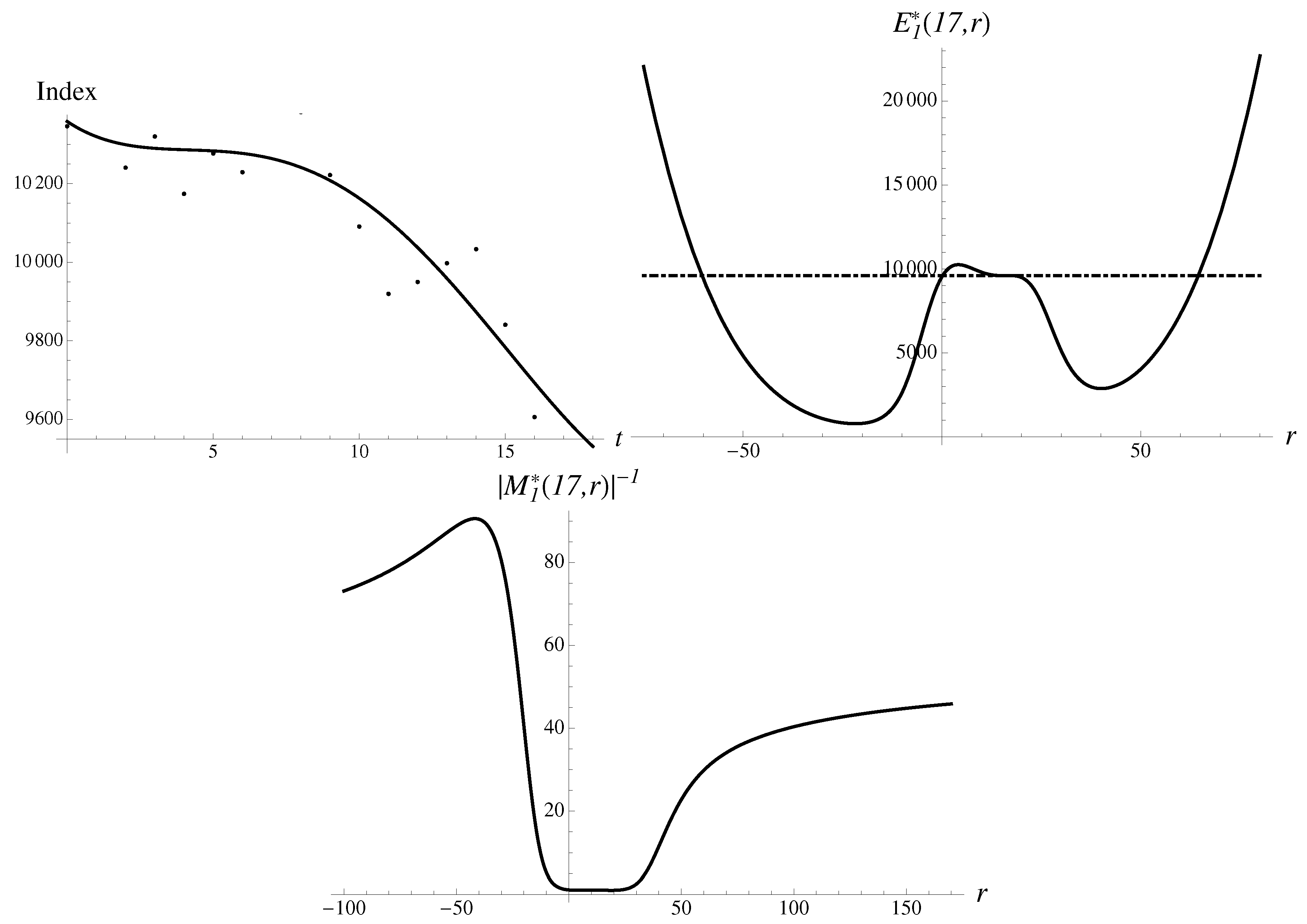
On 1 February 1917, Germany returned to the policy of unrestricted submarine warfare. The US market responded with a drop of 7.24% in Dow Jones, to $s_{17}=88.52$, from the value $s_{16}=95.43$. Soon, America goes to war. One might expect that the onset of a pandemic, pending war and terrorist attack will fit the same narrative, reflected in numbers and in almost identical market reaction, as illustrated in Figure 3. It demonstrates the data and the structural components, in striking resemblance to the two cases just considered above.

The most stable solution to Equation (14) could be extrapolated to the near future with the following results,

$$E_1^{*}=89.0437,M_1^{*}=0.0105049,$$

with an error of just $0.59\%$. There is also a less stable “upward” solution,

$$E_1^{*}=104.611,M_1^{*}=0.0405037.$$

There are also a couple of metastable solutions in between, with multipliers ∼1. The logistic approximant also gives rather good extrapolation numbers,

$$L=88.8922,M_L=0.00589679,$$

with the error equal to just $0.42\%$.

3.3. Fukushima, or Godzilla Strikes Again

Let us evaluate how Japan’s Nikkei stock index reacted to the triplet of earthquake, tsunami and nuclear crisis on 11–15 March 2011.

On Friday, 11 March, an earthquake struck and tsunami hit the coast of Japan, and over the weekend an explosion and radiation leaks were reported. The first trading day, on 14 March, saw a big drop of 6.18% in the value index, from the value of 10,254.43 to 9620.49. The second stage, on 15 March, Tuesday, brought a crash of 10.6% to the value of 8605.15, as fears of a nuclear crisis unfolded. All appearances and calculations for the first day drop are standard and are quite accurate, for $N=15$. Already, $E_1^{*}\left(16\right)=9600.25$ is good, with an error of just 0.21%. In addition, the data, multipliers and approximants look very similar to the second stage.

Consider the second stage, the crash, in more detail. In Figure 4, the data and the structural components are demonstrated, in striking resemblance to the cases just considered above.

The most stable solution to Equation (14) extrapolates to the following numbers,

$$E_1^{*}\left(16\right)=8922.19,M_1^{*}\left(16\right)=0.0115742,$$

with an error of $3.68\%$. There is also a less stable solution,

$$E_1^{*}\left(16\right)=\mathrm{10,544.3},M_1^{*}\left(16\right)=0.0303566,$$

pointing upward. In addition, there are two metastable solutions in between. The second-order Gompertz approximant gives rather good extrapolated numbers,

$$G\left(16\right)=8688.45,M_G\left(16\right)=0.00159094,$$

The numerical error brought by the Gompertz approximant equals to a small $0.97\%$.

3.4. Flash Crash

Sharp intraday movements can lead to the so-called flash crashes [37,38]. Such ultra-fast extreme events are so unexpected that they sometimes are equated with an ultra-fast black swan [38]. We believe that some features of the flash crashes may still be subject to symmetry considerations.

In particular, their magnitude could be captured based on the same type of information input and self-similarity technique as all other crashes. Or is it required to incorporate a shorter time scale and apply some modified methods?

Indeed, consider the famous flash crash of 6 May 2010. There were two stages of the price evolution. The first stage corresponded to the DJ index super-fast decline from the value of $s_{15}=$ 10,868.1, to the value $s_{15+3/4}=9869.62$, happening in the late afternoon and corresponding to the crash of 9.19% by magnitude, and the second stage of a fast recovery to the closing price $s_{16}=$ 10,520.3, with a relatively modest resulting final drop of 3.2%. Thus, there are two numbers to explain.

In Figure 5, the data and the structural components are demonstrated, in striking resemblance to the cases just considered above.

In a bit of a surprise, the probabilistic pattern preceding the flash crash is identical to the previous examples. The most stable solution corresponding to the lower bound gives the following estimate,

$$E_1^{*}\left(16\right)=\mathrm{10,277.1},M_1^{*}\left(16\right)=0.0125472,$$

with an error of $4.13\%$ compared to the bottom value of $s_{15+3/4}$. It is also about 3-times less stable, but still a rather stable solution pointing upward. The averaging over all (four) solutions in the discrete spectrum gives the result ${\overline{E}}_1\left(16\right)=$ 10,675.5, with a reasonable accuracy of $1.48\%$, compared to the value of $s_{16}$. The combined action of the two most influential solutions (groups of traders?) gives rather reasonable accuracy. One can deduce the meaning of such an exemplary performance of the average: as the dominating contribution was equivalent to panic selling caused by some technical reason, there was delayed minority buying, as well as some much less influential groups acting on a belief that the market would stabilize around $s_{15}$. The technical error had the same effect as the external shocks in previous examples, exposing the lowest possible bound, by prohibiting buying orders. As soon as the technical problem was resolved, buying resumed and brought the price to the equilibrium defined by the weighted average of all solutions.

Using the same methodology, we obtain a good lower bound by applying the Gompertz approximant, i.e.,

$$G\left(16\right)=\mathrm{10,079.5},M_G=0.00173164,$$

The numerical error brought by the Gompertz approximant equals $2.13\%$, compared to $s_{15+3/4}$. The averaging over all (four) solutions gives the result $\overline{G}\left(16\right)=$ 10,637.1, with a reasonable accuracy of $1.11\%$, compared to the value of $s_{16}$.

3.5. Bubbles

Consider the case of a so-called price bubble. At first, the index is going up monotonously and then changes the direction rapidly at some point. Such a development unfolds fast [39]. We could find a number of almost perfect bubbles “living” for 15–20 days, exclusively in the data on Shanghai Composite, while failing to find a good group of examples for the US indices.

When the global symmetry of time invariance is broken, the bubble is born. Its end is notoriously difficult to pinpoint [40]. Even high probability may not lead to the immediate bursting of the bubble over some period of time.

Consider a $7.78\%$ crash on 30 April 1996. In Figure 6, an almost perfect monotonous growth is seen. The pattern, with a little stretch of the imagination, could also be called a hockey stick.

With $N=15$, there are the following data points available:

$$s_0=581.38,s_1=578.07,s_2=579.82,s_3=583.38,s_4=586.96,s_5=584.67,$$

$$s_6=590.85,s_7=593.38,s_8=600.28,s_9=618.12,s_{10}=613.97,s_{11}=623.77,$$

$$s_{12}=664.65,s_{13}=652.67,s_{14}=707.61,s_{15}=738.62.$$

Moreover, the drop to the value of $s_{16}=681.16$ is to be “predicted”.

We are going to discuss below the results for the quadratic, cubic and quartic regressions. In such a way, one can appreciate the pattern’s evolution with increasing the order of regression.

3.5.1. Hockey Stick Bubble: Second Order

For the data given above, we find

$$s_{0,2}\left(t\right)=586.172-5.23371t+0.90299t^2.$$

The inverse absolute value of the first-order multiplier is shown in Figure 7. The first-order approximant is presented here as well. There is a typical probabilistic structure with two humps in the multiplier dependence on r.

The integral representation for the continuous spectrum could be calculated as well and the extrapolation is given as $I(16,86.8181)=732.002,$ with a relative percentage error of $7.46\%$. The result generated by the most stable solution in a discrete spectrum is given as follows,

$$E_1^{*}(16,-74.3412)=721.55,M_1^{*}(16,-74.3412)=0.120949,$$

with a numerical error of $5.93\%$. We also found a less stable solution pointing upward. Both methods give qualitatively correct results.

3.5.2. Hockey Stick Bubble: Third Order

For the data given above we find

$$s_{0,3}\left(t\right)=577.928+3.34243t-0.682388t^2+0.0754942t^3.$$

The inverse absolute value of the multiplier behaves qualitatively differently than in the previous example, as shown in Figure 8. A similar statement holds for the first-order approximant. There is only one dominating hump in the multiplier dependence on r, strongly skewed to the right.

The integral can be calculated taking into account that the region of integration is limited from the left and it is the upper integration limit that ought to be optimized. The integral equals $I(16,30.2579)=786.899,$ pointing upwards and in the wrong direction. The result given by the most stable solution equals

$$E_1^{*}(16,38.1776)=793.7,M_1^{*}(16,38.1776)=0.202898,$$

which also points in the wrong direction. There is also a less stable solution pointing upward. Yet, from the standpoint of stability, the second-order solutions are better than the third order.

3.5.3. Hockey Stick Bubble: Fourth Order

For the data given above, we find

$$s_{0,4}\left(t\right)=581.36-3.7571t+1.78459t^2-0.204487t^3+0.00999933t^4.$$

Integral (13) can be calculated numerically, with the sough extrapolation given as $I(16,57.9116)=682.93,$ with a relative percentage error of just $0.26\%.$

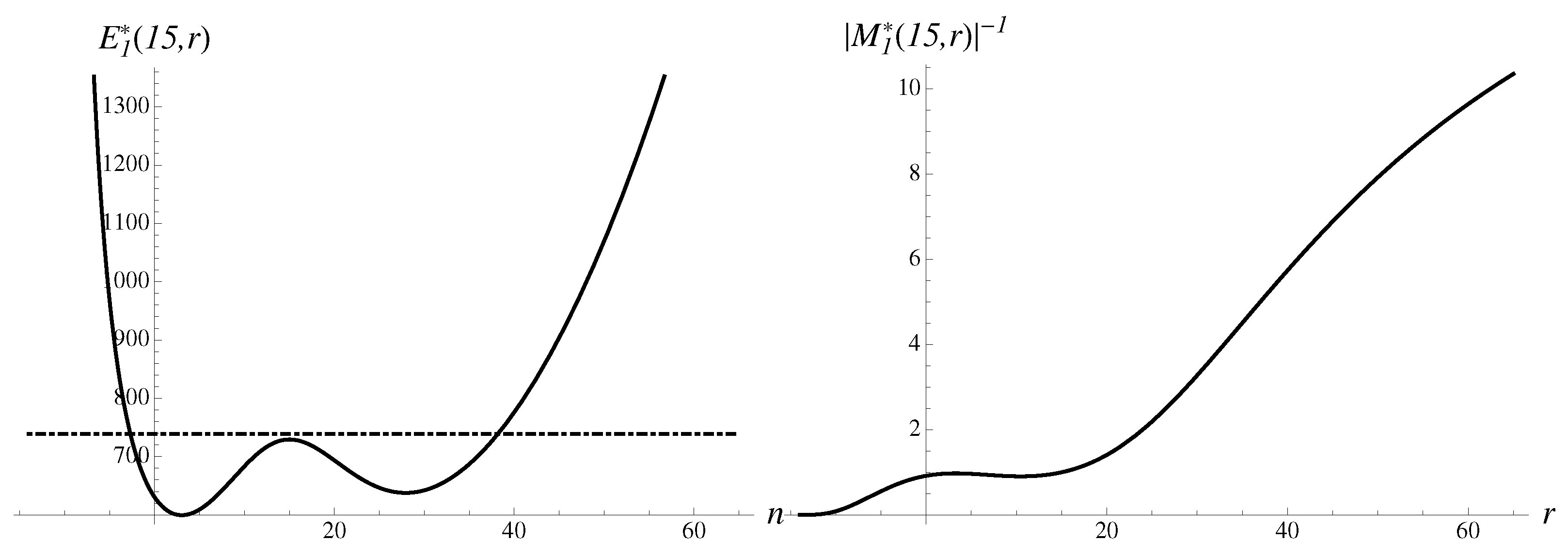
Let us analyze the components contributing to the integral. The inverse multiplier of the first order is shown in Figure 9. The first-order exponential approximant is presented here as well.

There are two very asymmetric probabilistic humps in the inverse multiplier.

The second method finds the solutions in a discrete spectrum to Equation (14). The most stable solution gives

$$E_1^{*}(16,-48.1034)=685.608,M_1^{*}(16,-48.1034)=0.00844428,$$

with a very small error of $0.65\%$. An upward solution appears much less stable, with

$$E_1^{*}(16,34.2447)=836.417,M_1^{*}(16,34.2447)=0.103455.$$

There are also a couple of additional solutions located in between with much larger multipliers ∼1, although such solutions carry little weight and do not contribute to the averages much. However, in real time such solutions may still show up under special conditions.

From the stability standpoint, the fourth-order solutions are better than in the third order, suggesting that downward solutions will be more probable than upward.

The second-order super-exponential approximant (11) gives

$$E_2^{*}(16,-102.776)=669.048,M_2^{*}(16,-102.776)=0.00132161.$$

The numerical error brought by the super-exponential approximant (11) is $1.78\%$. Similarly, the Gompertz approximant gives the following estimate

$$G(16,-111.248)=667.12,M_G(16,-111.248)=0.00108169,$$

with an error of $2.1\%$. The logistic approximant gives

$$L(16,-59.9771)=684.40,M_L(16,-59.9771)=0.0047201,$$

with an error of just $0.47\%$.

We observe that, for the hockey stick bubble, symmetric $E_1^{*}$ and logistic approximants give better results than approximants with broken symmetry. Compared to the original fourth-order regression, which gives the error of $15.9\%$ and predicts the wrong direction, the improvement appears to be significant.

In the most stable case of the fourth-order theory, the examples of crashes considered above give very similar patterns in the probabilistic sense, despite their original data sets being very different. We are unable to verify that any external shock caused the bubble burst, but we may very well suspect it by analogy. In the examples below, we consider only the fourth-order models, since the models of lower orders turned out to be less stable.

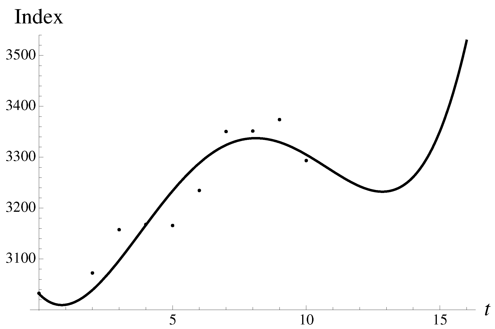
3.5.4. The Largest Bubble

Consider, in the fourth order, the largest so far and known to us, a drop in the Shanghai Composite index, with a magnitude of $16.4\%$, to the value of $s_{16}=750.3$. It occurred on 23 May 1995. The year 1995 saw a deteriorating relationship between China and the rest of the world. Loans from Hong Kong seized and the Chinese economy stalled. May 1995 saw a halt to treasury bond futures trading, after a price manipulation scandal in February 1995.

We think that the magnitude of the drop is important, because it is more difficult to ascribe the severe crash to some noisy outburst [7], while much smaller moves/crashes can be influenced by noise.

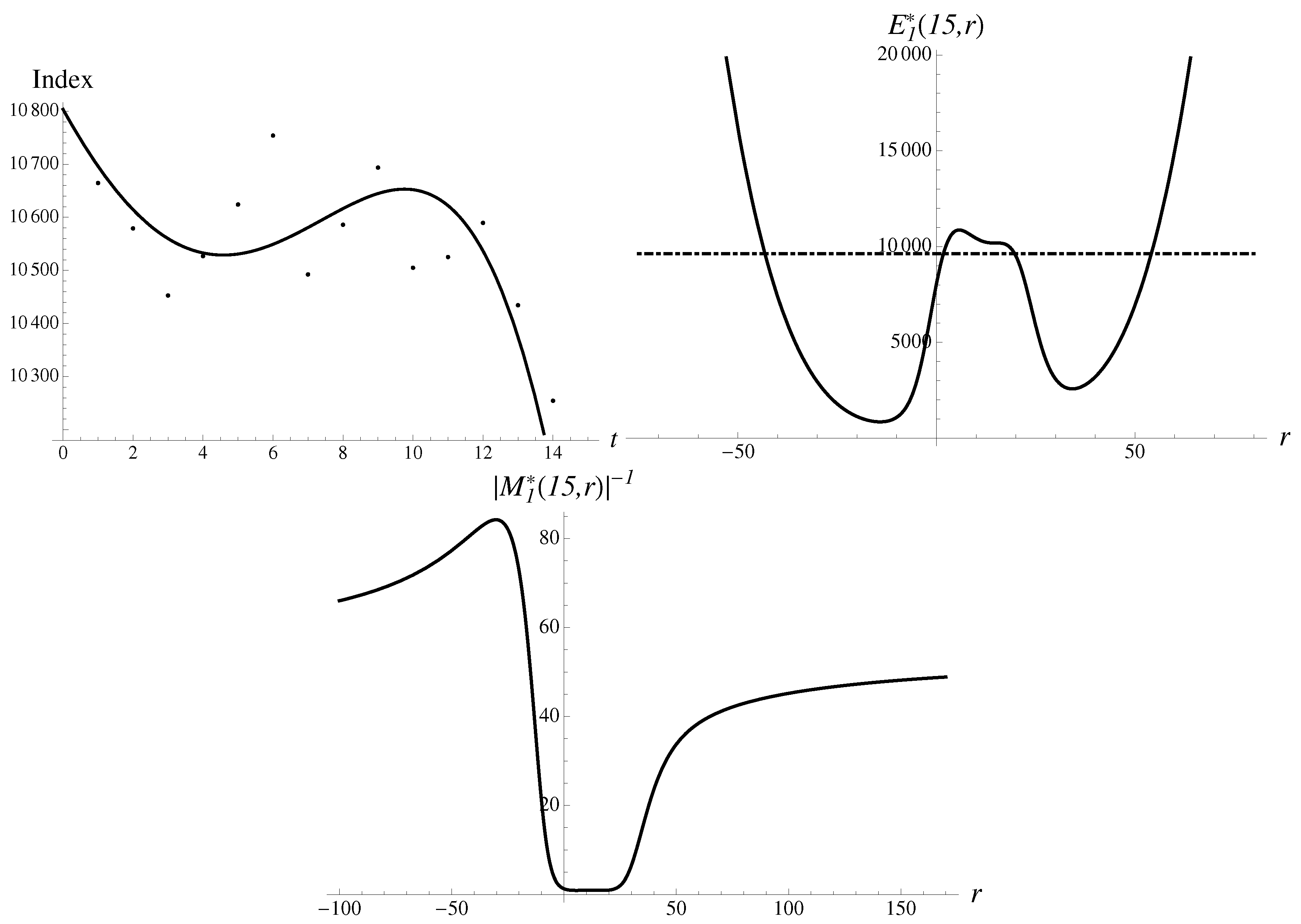
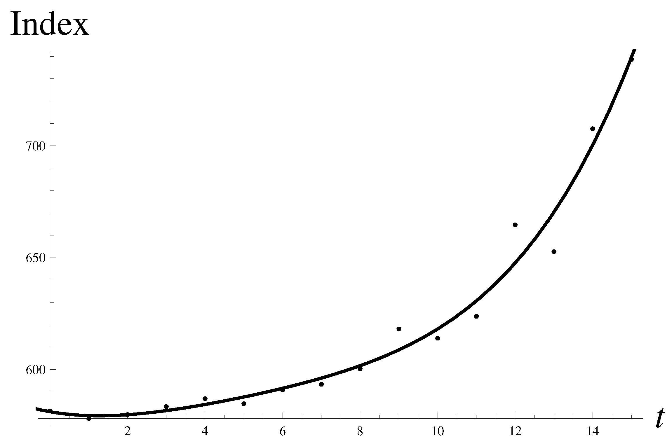
It is always helpful to look at the original data and compare them to the quartic regression. There is almost monotonous rapid growth as can be seen in Figure 10.

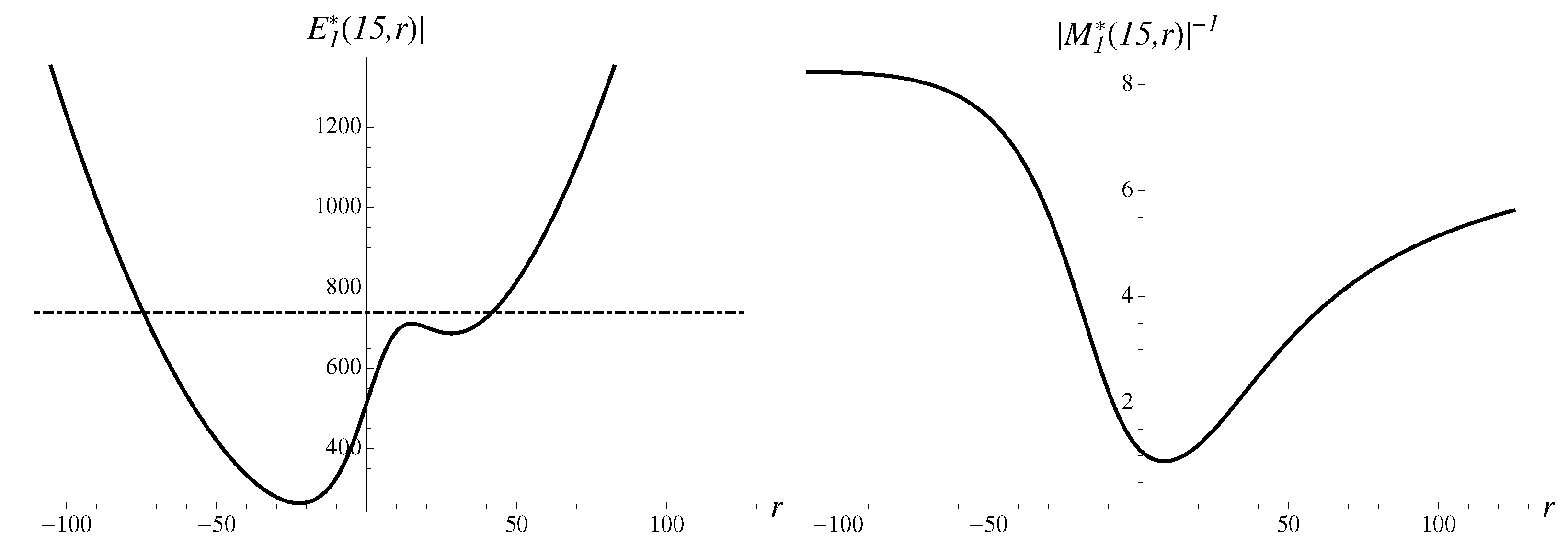
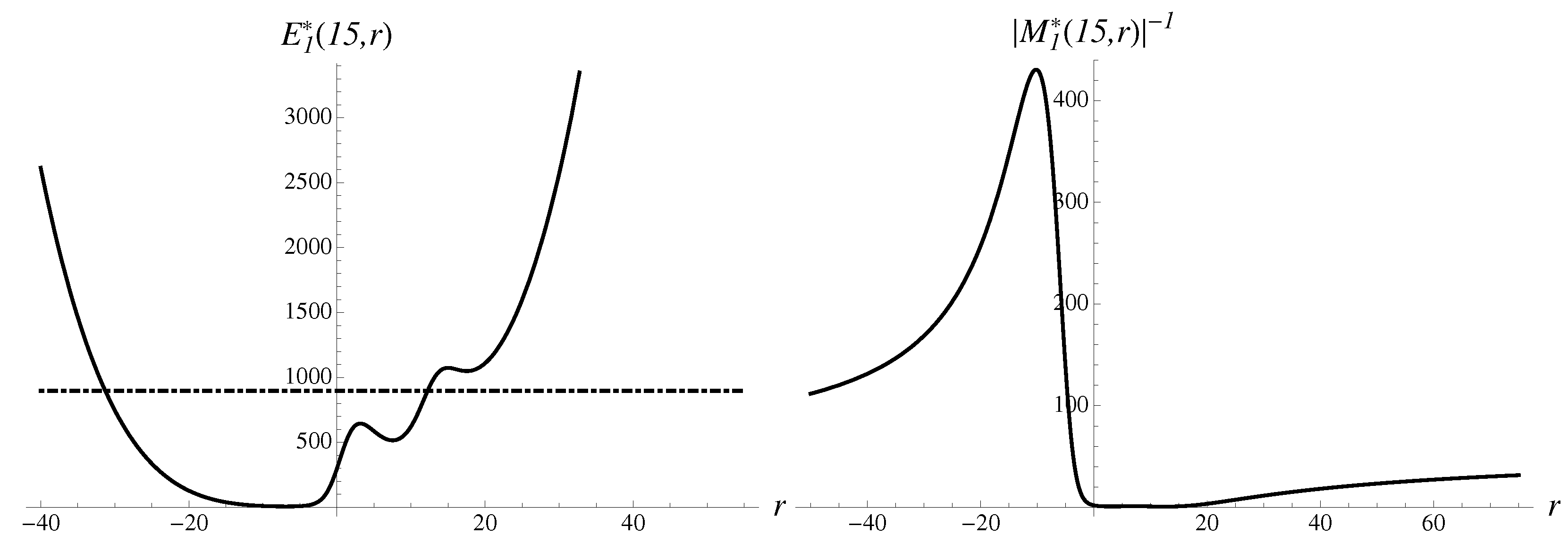
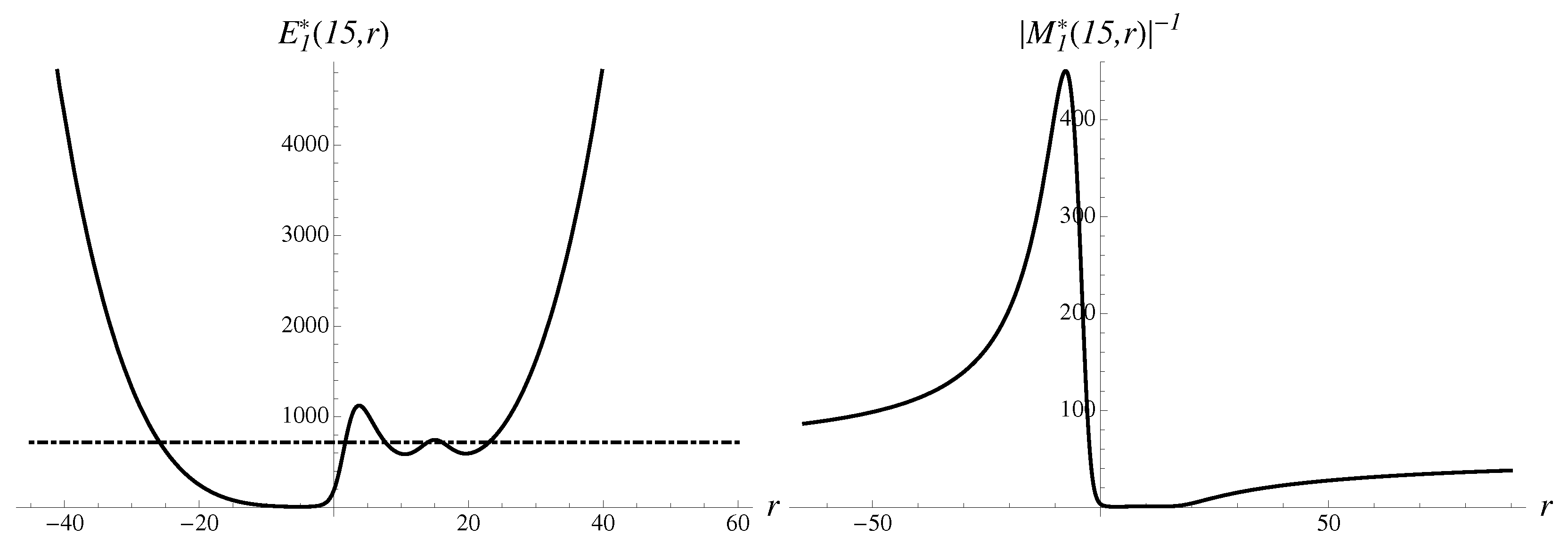
Let us analyze the structural components contributing to the integral. The first-order inverse multiplier is shown in Figure 11. The first-order approximant is shown as well.

There are two very uneven probabilistic humps in the inverse multiplier, suggesting that the region of large negative r dominates. The forecast by integration method expressed by Equation (13) is equal to $I(16,41.2538)=762.326,$ with an error of $1.6\%$.

In the discrete spectrum, the most stable downward solution gives

$$E_1^{*}(16,-31.2853)=803.998,M_1^{*}(16,-31.2853)=0.00552808,$$

with an error of $7.2\%$. However one can also find an unstable solution pointing upward, i.e.,

$$E_1^{*}(16,12.2433)=1007.785,M_1^{*}(16,12.2433)=1.54605.$$

There are no additional metastable solutions, and nothing can theoretically prevent the strong move. Approximant (11) gives the result $773.847$, while the Gompertz approximant gives the estimate $770.287$, with an error of $2.7\%$. The logistic approximant is also qualitatively correct and gives an error of $6.9\%$. Thus, the methods with broken or partially restored symmetry perform better.

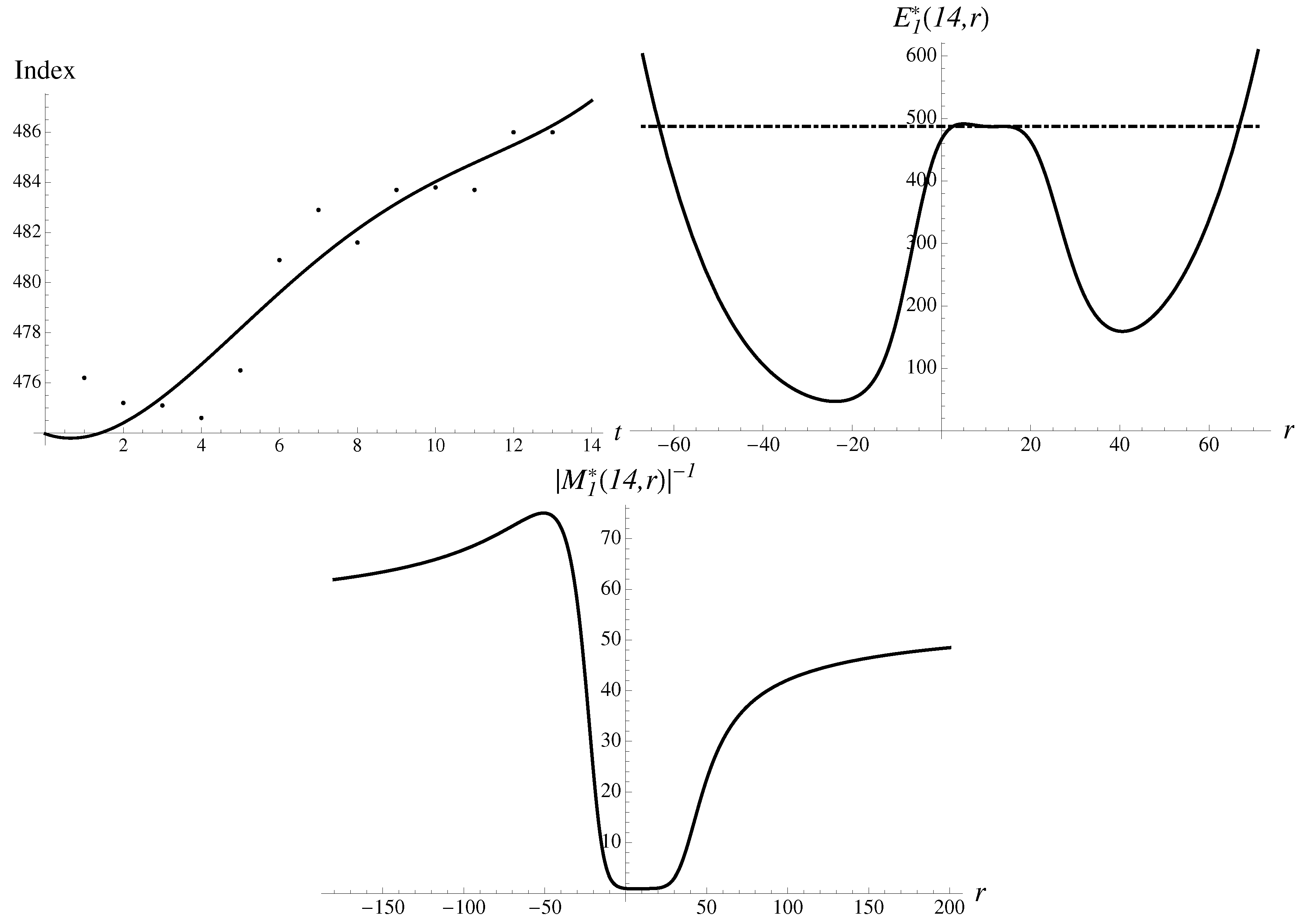
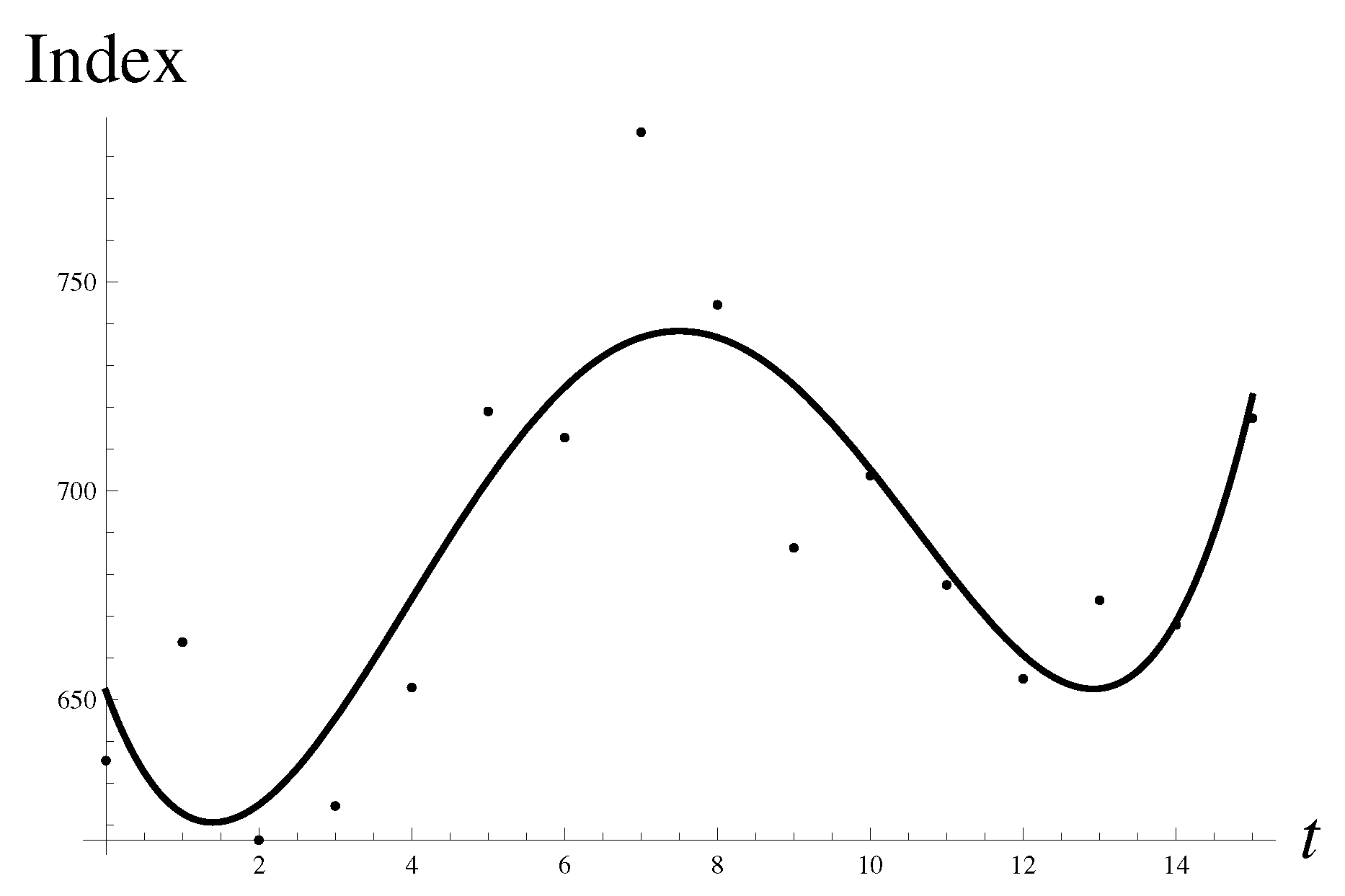
Curiously enough, we were able to find an almost identical bubble on 9 August 1994, with a drop in price of 12.7%, $N=16$, $s_{16}=711.8$ and $s_{17}=621.58$. To appreciate the analogy, see Figure 12 for more details.

The first-order approximant gives the result 662.347, with an error of 6.6%. Calculations with the Gompertz approximant give the estimate $644.031$, with an error of $3.61\%$.

3.5.5. Death of the Hero

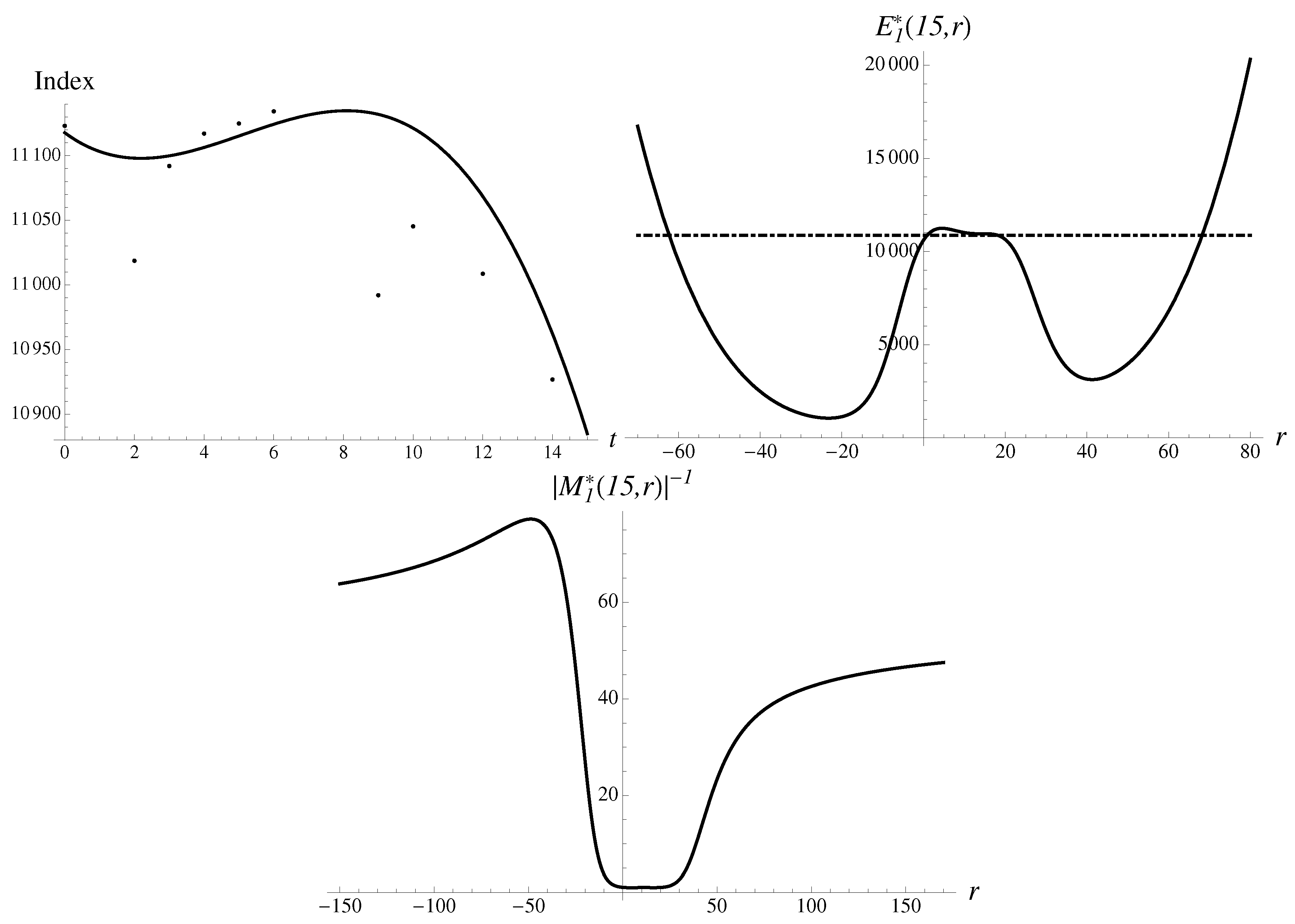
On 19 February 1997, the burst of the bubble was triggered by the death of Chinese leader Deng Xiaoping. The drop of Shanghai Composite was quite significant and amounted to 8.91%, from $s_{15}=982.4$ to $s_{16}=894.85$. Figure 13 demonstrates the data and the scenarios.

There are again two uneven probabilistic humps. The most stable solution points downward, with the following results,

$$E_1^{*}(16,-64.3744)=931.32,M_1^{*}(16,-64.3744)=0.0136826,$$

with an error of $4.07\%$. There is also a quite stable upward solution, with

$$E_1^{*}(16,79.6362)=1042.18,M_1^{*}(16,79.6362)=0.0233068.$$

There are also two less stable solutions in between. The average over all four scenarios gives the following result, ${\overline{E}}_1\left(16\right)=972.567,$ which is not indicative of any significant movement and anticipates fast recovery the very next day. The trigger/shock again was likely to act to select the downward solution, effectively prohibiting the stable upward solution.

Analogous calculations with the Gompertz approximant give the following estimate

$$G(16,-146.322)=914.401,M_G(16,-146.322)=0.00196998,$$

with an error of $2.18\%$.

Similar behavior of the DJ index was observed when, on Saturday, 24 September 1955, the US president Eisenhower had a heart attack. The next Monday, the Dow index plunged by 6.5% to the value of $s_{15}=455.6$. The case of “hero in mortal danger” is practically a twin case of the bubble just discussed above. With $N=14$, in the fourth order we arrive to practically the same patterns, as shown in Figure 14, with all known-to-us approximants bringing accuracy close to 1%, with the Gompertz approximant being the best, giving

$$G\left(15\right)=452.336,M_G\left(15\right)=0.00177325,$$

with an error of just 0.72%.

The bubbles discussed above are characterized by similar stable downward solutions but differ in the relative contribution of a competing upward solution. In principle, when the competition is allowed to unfold, a possible crash and melt-down may compensate for each other, unfolding in parallel.

Sometimes, there is an explicit bailout buying, designed to compensate for the imminent crash. The case of the LTCM bailout on 23 September 1998 is well documented and analyzed in great technical detail. There was an actual, widespread fear of a catastrophic chain reaction of liquidations throughout the global financial system. The case is discussed as the example of a correct binary forecast, nevertheless leading to ruin [5]. However, in fact, the DJ index dropped by only 1.87%, from $s_{15}=8154.4$ to $s_{16}=8002$.

The case has a very similar temporal structure and structural components to the two bubbles discussed above. With $N=15$ and the fourth-order regression, we find

$$G\left(16\right)=7497.15,M_G\left(16\right)=0.00199696,$$

with an anticipated drop of 8.1%. However, taking the weighted average over solutions gives a very accurate estimate for actual behavior, i.e., $\overline{G}\left(16\right)=8017.48$, with an error of just 0.19%.

3.6. Non-Monotonous Crashes

Various non-monotonous situations could also result in large drops. The configurations of data points sometimes remind us of various patterns recognized by technical analysis.

3.6.1. When the Market was Young

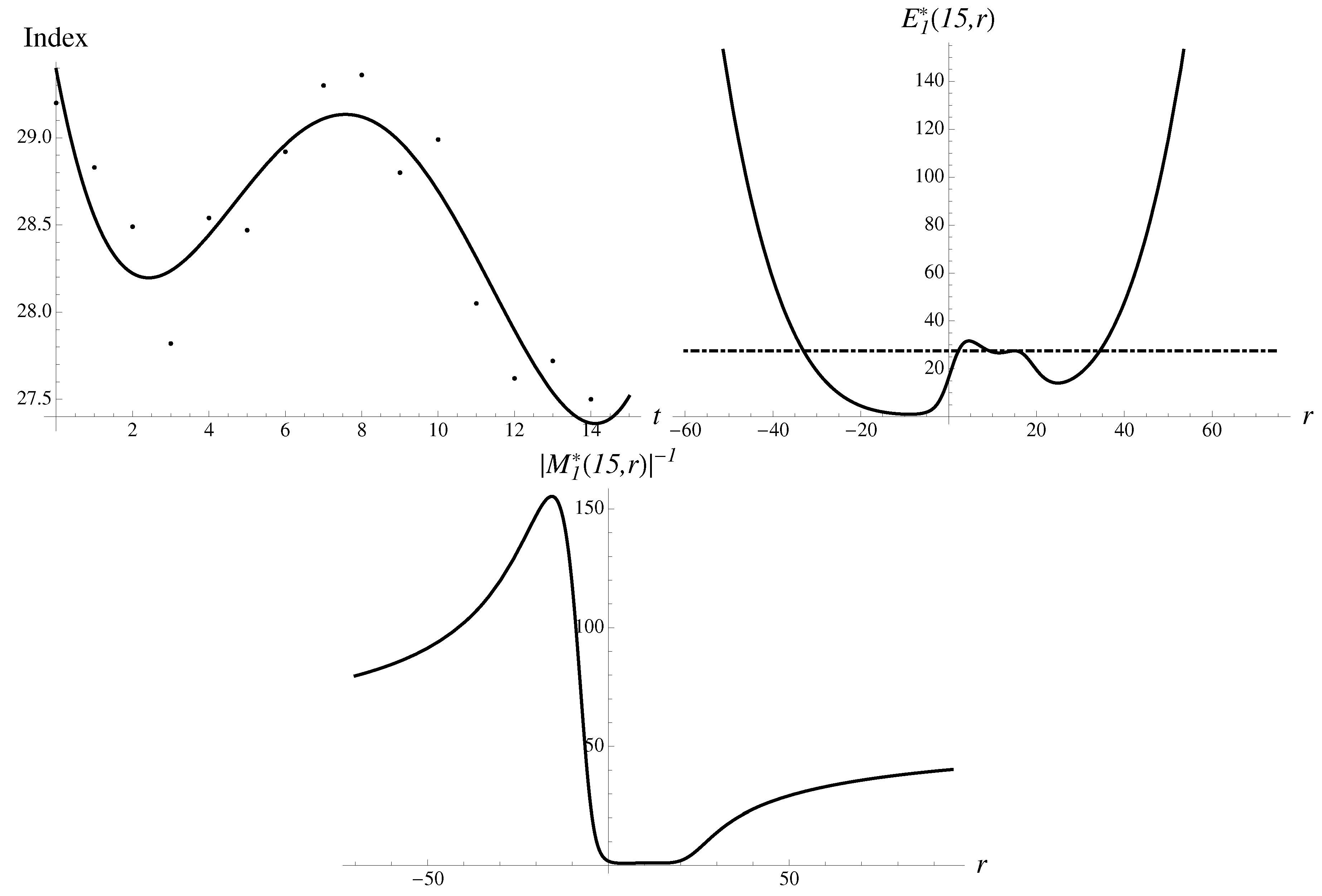
Consider the very first case of a crash, coined below “when Market was young”, corresponding to the first well-documented drop of 6.23% in the Dow Jones Industrial Average on 29 June 1896, just a month after the very index was created. Consider the typical for our study data set with $N=15$, with $s_{15}=27.44$ and $s_{16}=25.73$. We doubt that any other technique can describe the first crash.

One can safely assume that the traders of the time were not aware of the random walks, effective markets hypothesis, critical slowing down, log-periodic oscillations, etc. However, they definitely could plot, knew algebra and what is a return, and had the same human abilities as we enjoy today. They also knew how to panic, since the term “panic” was applied as a synonym of early crashes. There is no famous panic associated with the event, but it was only a precursor to the well-documented panic of 1896.

Figure 15 demonstrates the data and the components contributing to the integral.

There are again two very uneven probabilistic humps, and the region of large negative parameter r is dominant, carrying considerably more weight. The most stable solution in the discrete spectrum results in

$$E_1^{*}(16,-33.0239)=24.8664,M_1^{*}(16,-33.0239)=0.00800164,$$

and an error of $3.36\%$. In addition, there is also the solution pointing to the opposite direction,

$$E_1^{*}(16,34.40261)=31.9279,M_1^{*}(16,34.40261)=0.0615679,$$

but it appears to be less stable. In addition, there are four additional metastable solutions in between. The corresponding multipliers are close to unity. Such a multiplicity of solutions reflects the oscillatory nature of the data set.

In our investigation, we observed no more than six solutions $r_k^{*}$ forming the discrete spectrum. All solutions are presented in Figure 1.

The averaging in the discrete spectrum gives a much better result, ${\overline{E}}_1\left(16\right)=25.731$, with an impressive accuracy of $0.00385178\%$. The combined action of the two most influential solutions (groups) gives better accuracy. One can think that such an exemplary performance of the average occurred for the following reason: as the majority was panicking and selling, there was a cool-headed minority of bargain hunters buying or short sellers covering their short interests. Some much less influential (or less knowledgeable) groups acting on the belief that the market will stabilize around $s_{15}$ were also present.

3.6.2. Flag-like Growth

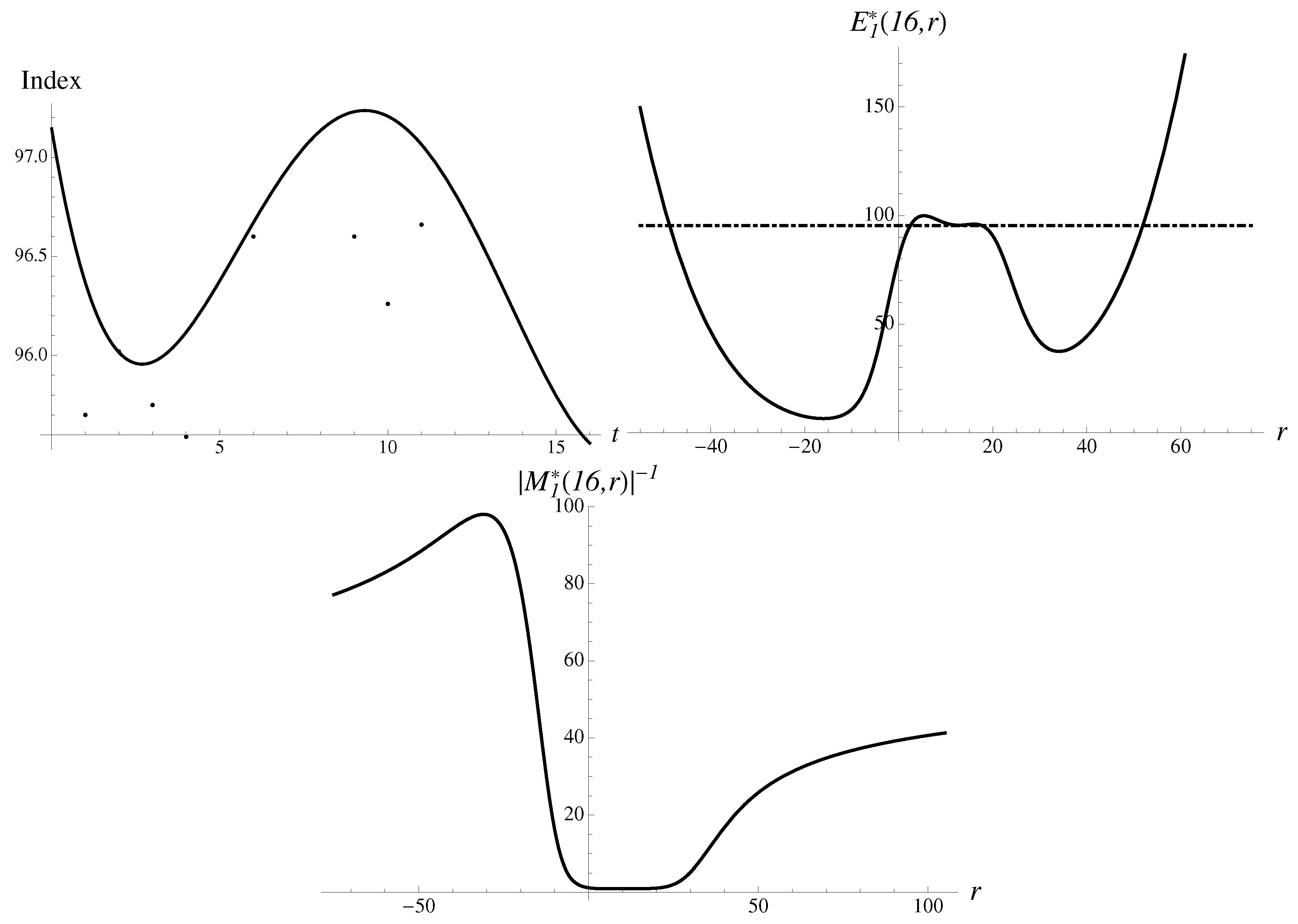
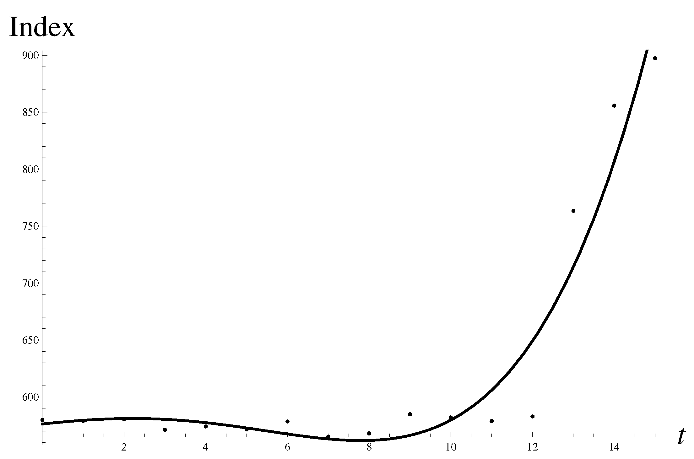
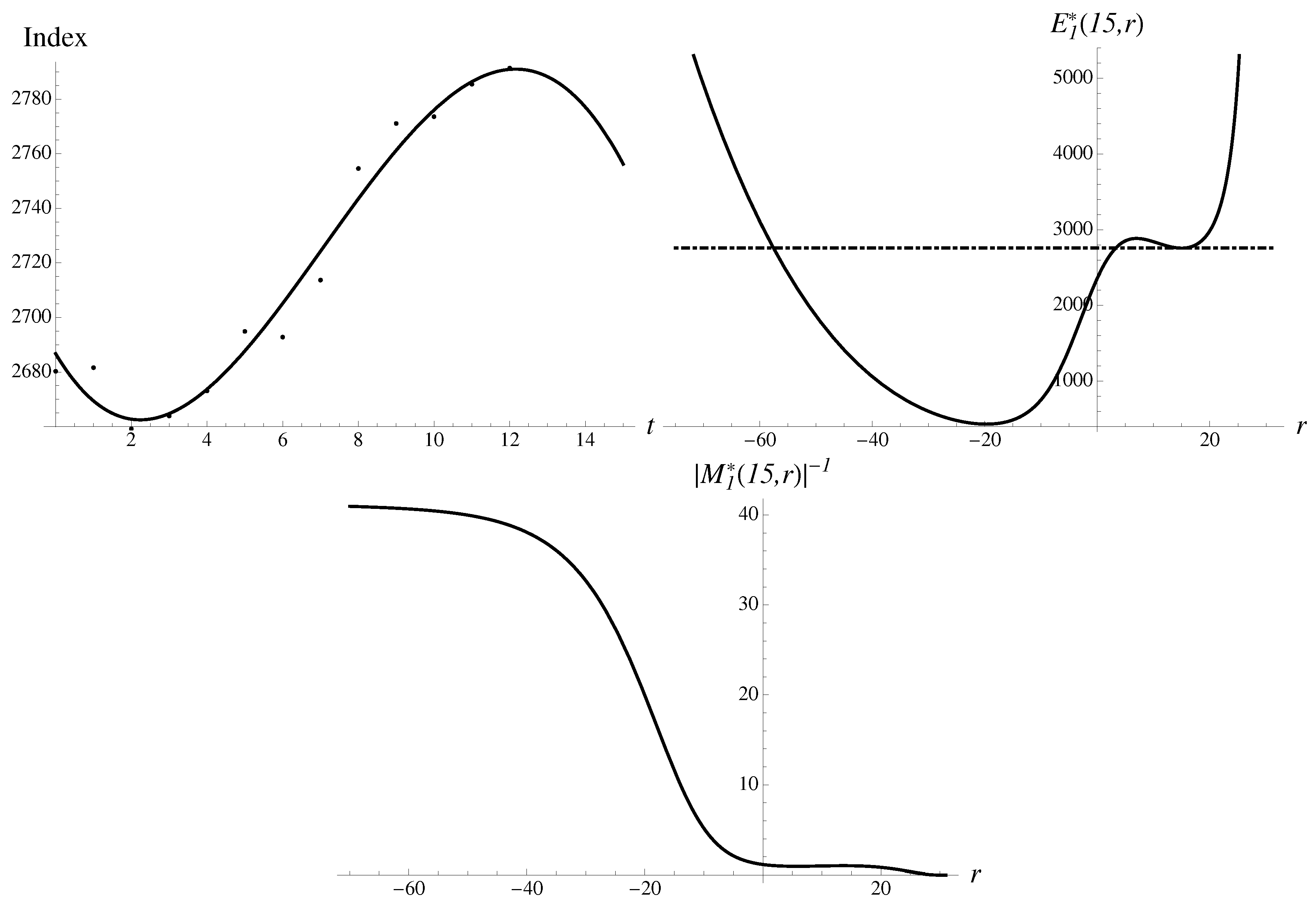
Consider again, only in the fourth order, the drop in the Shanghai Composite value of $7.7\%$ on 19 January 2015, to the value of $3116.35$. The futures market crashed even more, by a maximum allowed 10%, and trading was suspended on 19 January. The crash was preceded by a flag-like price pattern shown in Figure 16.

Let us show the data against the quartic regression. The non-monotonous growth can be seen in Figure 16.

Let us plot the now familiar structural components in Figure 17.

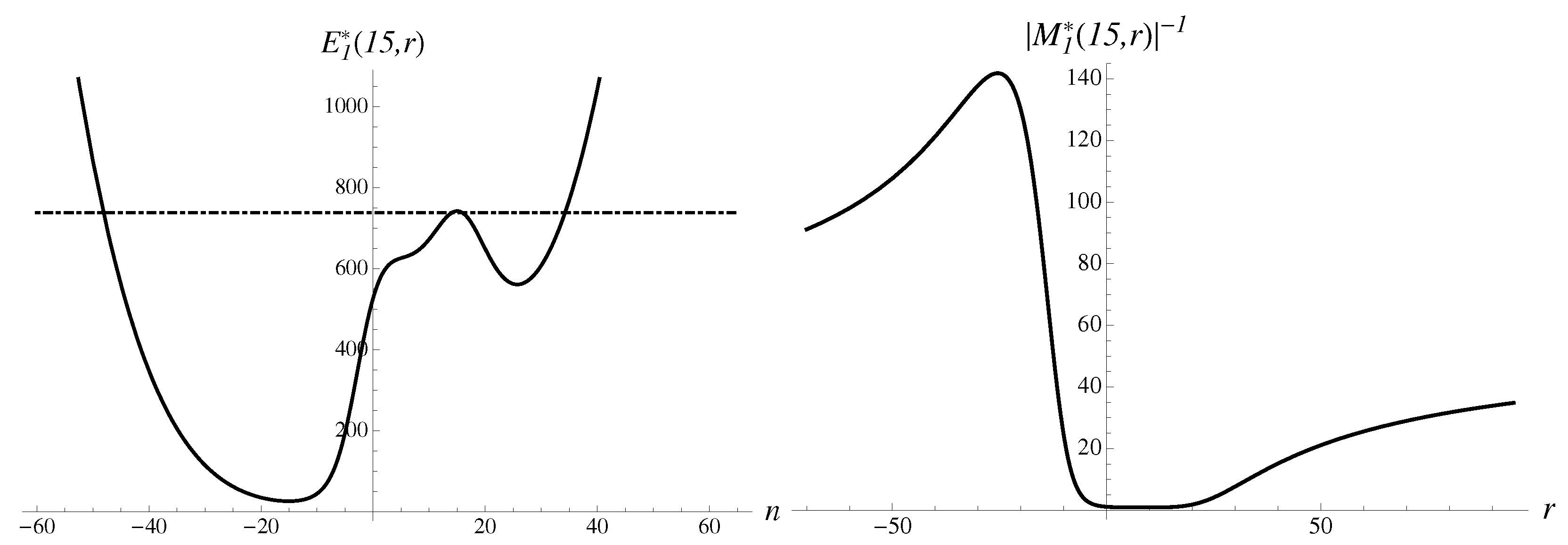
There are again two very uneven probabilistic humps, and the region of large negative r turns to be dominant, carrying considerably more weight. The suggestion obtained by integration method (13) is given as $I(16,48.2295)=3056.53,$ with a relative percentage error of $1.92\%$.

One can find the most stable solution to Equation (14), with

$$E_1^{*}(16,-36.283)=3077.94,M_1^{*}(16,-36.283)=0.00790401,$$

with an error of only $1.23\%$. The less stable “upward” solution can be found as well, with

$$E_1^{*}(16,35.8823)=3891.56,M_1^{*}(16,35.8823)=0.0594448,$$

in agreement with a naive, intuitive analysis. In addition, there are also a couple of less stable solutions with multipliers ∼1. The less stable solutions may show themselves in real time under special conditions.

The super-exponential approximant of the second order (11) gives

$$E_2^{*}(16,-79.955)=2984.44,M_2^{*}(16,-79.955)=0.00127141.$$

The numerical error brought by the super-exponential approximant (11) equals $4.23\%$. By applying the Gompertz approximant, we arrive to the following numbers,

$$G(16,-86.7103)=2973.58,M_G(16,-86.7103)=0.00104341,$$

with an error of $4.58\%$. Logistic approximation gives the result

$$L(16,-45.8111)=3071.16,M_L(16,-45.8111)=0.00444567,$$

with an error of $1.45\%$. Thus, both solutions with restored time-translation symmetry perform better.

3.6.3. Head and Shoulders Growth

Consider again, only in the fourth order, the drop in the Shanghai Composite value of $7.05\%$, to the value of $s_{16}=666.77$, which happened on 4 November 1994. The crash was preceded by a head-and-shoulders-like pattern shown in Figure 18. Let us compare the data to the quartic regression. There is an oscillatory growth pattern as can be seen in Figure 18.

Let us plot the components contributing to the integral, as shown in Figure 19.

There are again two very uneven probabilistic humps. The region of large negative r is dominant and carries considerably more weight. The most stable solution to Equation (14) is found as follows,

$$E_1^{*}(16,-25.8732)=633.697,M_1^{*}(16,-25.8732)=0.0055577,$$

with a numerical error of $4.96\%$. One also finds a less stable “upward” solution

$$E_1^{*}(16,23.0463)=924.701,M_1^{*}(16,23.0463)=0.167126.$$

There are also several solutions in between, with multipliers ∼1. Such a multiplicity of solutions reflects the oscillatory nature of the data set. The averaging in the discrete spectrum gives a much better result, ${\overline{E}}_1\left(16\right)=659.47$, with an error of $3.18\%$. The logistic approximant shows an accuracy of $5\%$. The remaining methods give much worse results, with an accuracy of 9–10%. Thus, all solutions contribute to the best result, and such situations can be considered as corresponding to endogenous development, in the absence of exogenous shocks.

3.6.4. Friday the 13th Bad Luck

We would like also to discuss briefly the case of a crash due to self-generated nervousness [14,33]. It is much harder to discern, since market watchers tend to come up with plausible economic rationalizations. See, for instance, the case of a mini-crash in the DJ index, of 6.9% on Black Friday, 13 October 1989. It was blamed on the news of a UAL leveraged buyout, while the majority of the market professionals were not aware of the fact (Feltus, Shiller). Likely, it was a case where sentiment overcame the criteria of value, and the market experienced a wild swing.

The price pattern preceding the crash reminds us of the shallow cup with a long handle. With $N=15$ and $s_{16}=2569.3$, the pattern and distributions can be found, as shown in Figure 20.

There is marked asymmetry in the probabilities for downward movement (very high) and upward movement (negligibly low). The most stable solution to Equation (14) gives

$$E_1^{*}(16,-57.5812)=2622.53,M_1^{*}(16,-57.5812)=0.023424,$$

with an error of $2.07\%$. By applying the Gompertz approximant, one can obtain an even better estimate,

$$G(16,-132.884)=2579.44,M_G(16,-132.884)=0.00437036,$$

with an error of $0.39\%$. Indeed, self-generated nervousness has the same overall effect as exogenous shock.

4. Comments on Trading

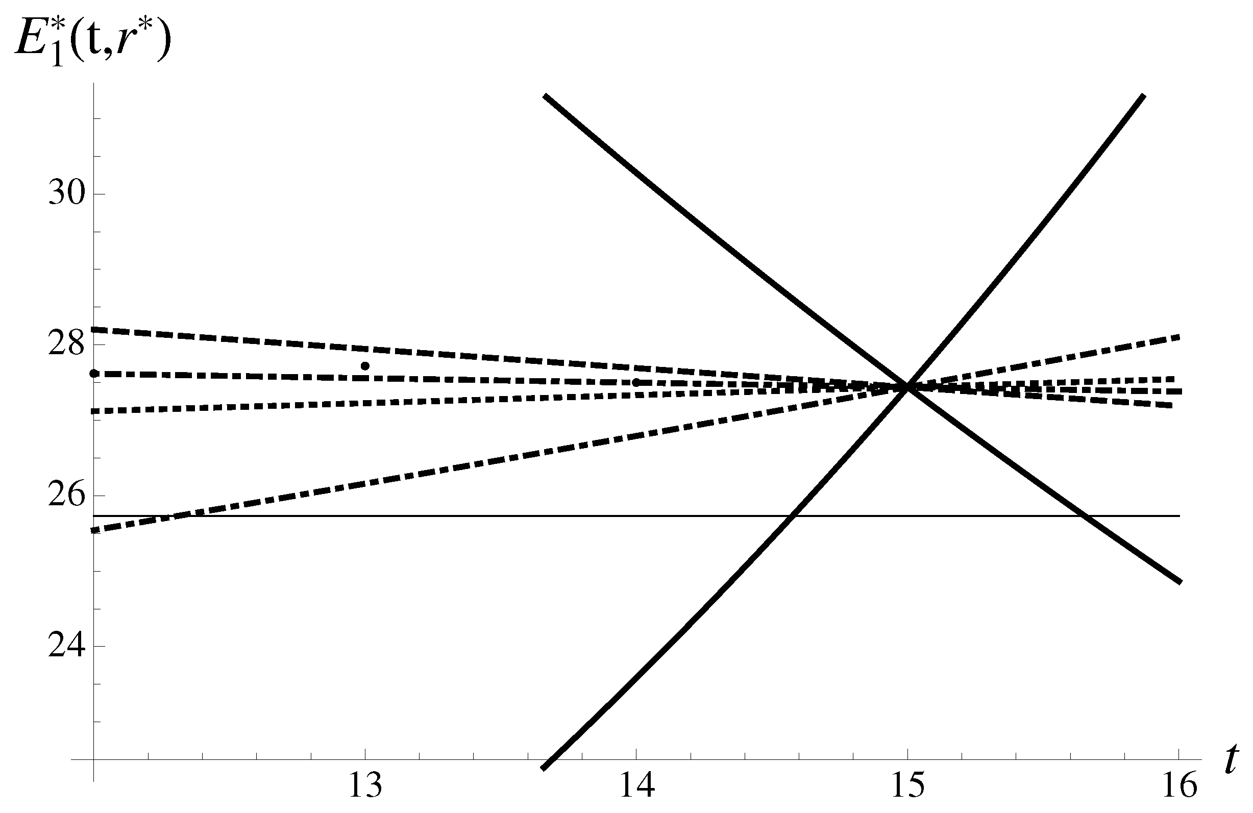
Sensible theory should help to understand why making predictions, and in particular about the future, is so hard. Our understanding is as follows. Instead of a unique solution to the problem, we are confronted with multiple solutions, as illustrated in Figure 1. The solutions are endowed with different strengths determined by multipliers. In our view, the price evolution is not reduced to reaching the most stable solutions, but various metastable solutions can come to existence as well. Such possibilities complicate actual prediction.

In real life, traders are using bounds to make a certain bet(s), calling them support (lower bound) and resistance (upper bound). The determination of support and resistance levels is performed several times in the course of day trading. Depending on the actual value of the price index, our spectrum of discrete scenarios, or poor man’s order book, gives a priori estimate for possible support and resistance levels, with the direction of bet toward the more stable bound, suggested by the relative stability of the bounds.

In such a trading method, we only calculate probabilities for the price going up or down and corresponding levels. They are supposed to replace the true proportion of buy and sell orders. If in the course of trading some of the bounds are crossed, one may as well issue a new set of levels and probabilities.

One may attempt to profit not only from the knowledge of the most stable solutions or weighted averages, but also from the knowledge of metastable solutions. The latter could be understood as violations of the overwhelmingly natural principle of maximum stability, akin to violations of ergodicity over observation time scales.

Should one even try to give a unique forecast? In fact, looking at and analyzing the typical picture of scenarios emanating from the last known price, shown in Figure 1, one should have at least two plans for action, depending on which set of bounds is going to be preferred, because of the arrival of actual-life new information, not captured by the model. Skipping scenarios in the middle and considering only trading in broad bands may lead to some sort of a barbell [5], bi-modal (tri-modal?) trading strategy.

The market breaks down/crashes because many traders chase a single opportunity and use similar strategies to do so. Strategic crowding can cause an abrupt phase transition from smooth behavior into a regime prone to sharp price movements [34]. Anecdotally, it seems to be the mechanism in the couple of drawdowns in the US equities markets of 2018. The crowding was thought to be not purely dynamical, but state-dependent, meaning that many hedge funds had all built up large positions in a few well-known names (Alphabet, Facebook, Amazon, etc.). Moreover, different trading teams within the same funds frequently found themselves concentrated in these few names. This resulted in the undermining of the usual modeling assumption that the different teams’ positions are independent. Such a concentration of positions in a few names is known as “crowding”, and the result is that if one of these big positions has to be liquidated, there may not be any substantial buyers left, which means prices have to drop substantially for willing buyers to emerge. Instead, the selling by one of the funds may precipitate more widespread selling, since the “mark-to-market” positions decline and some funds may choose to rotate out of these losing names. The most significant reason for selling is deleveraging. A drop in the mark-to-market valuation causes a margin call by the lender, which a fund may not be able to meet very easily and has to sell the position, precipitating a further and wider unwinding. In particular, the deleveraged names suddenly have higher volatility and risk control demands liquidation. The set-up resembles a self-organized process and the unwinding sounds like an avalanche. Self-similarity seems like a natural description of the unwinding process. The mechanisms of deleveraging by many of the big market participants are often part of the big picture of the crash. The idea was expressed by Dr. Dmitrii Karpeev, in private communication.

5. Conclusions

We introduce a general framework for quantitative technical analysis of market prices with exclusive attention to the concept of replica symmetry and global time-translation invariance and their spontaneous violation and restoration. Such an approach allows the determination of probabilistic trading patterns as a result of a local breakdown of replica symmetry. It turns out that different temporal patterns, such as bubbles, hockey sticks, etc., have very similar probabilistic distributions before a crash. One can also give a quantitative estimate for the magnitude of a crash.

Within the discrete spectrum of the origins found from the solution to optimization problems, one finds the solutions of two types. Normal solutions tend to follow the data rather closely. In addition to normal solutions, we found anomalous solutions adhering to the data rather loosely, but they appear to be very stable. Anomalous solutions correspond to crashes. A typical discrete spectrum of solutions with normal and anomalous solutions is shown in Figure 1. The terminology, of course, is borrowed from the theory of superconductivity, where anomalous solutions play the key role.

After some manipulations concerned with handling of the broken/restored replica symmetry and global time invariance, we arrive at the exponential solution for the price with an explicit finite time scale, not unlike the celebrated Meissner–Higgs mechanism of generating some typical space scale (see, e.g., paper [35]). The symmetries involved in the two phenomena are of a different nature, but in both cases a fundamental mechanism of broken symmetry is involved. Technically, in the field theory it is accomplished by breaking the so-called global gauge symmetry to a local gauge symmetry.

The new method of quantitative technical analysis might possibly help to improve the investment strategies of stock market players. We point out that it is possible to actually develop a trading strategy based on a projection of a discrete spectrum of probabilistic scenarios. We note that traders are often using bounds to make a certain bet(s), calling them support (lower bound) and resistance (upper bound). The determination of support and resistance levels is performed several times in the course of day trading. The spectrum of discrete scenarios gives a priori estimate for such levels, with the direction of the bet suggested by the relative stability of the bounds, expected to move towards a more stable level.

When the most stable solution points to a strong move down and is significantly more probable than all others, one should consider issuing a hazard signal, akin to a seismic hazard. The signal may very well persist over some period of time. Moreover, if someone would intend to stabilize the market in such conditions, it may be possible to act by pushing it away from the most stable solution and to the region of metastable solutions. We note that there are some rather interesting empirical approaches to binary indicators for self-organized crashes, based on market mimicry/stocks co-movement [33] or on a critical slowing down analogy with critical phenomena [41].

We attempted to show that panics of an old and crashes of a new era have very similar explanations. The analogous description follows from the standpoint of replica symmetry and time-translation symmetry, which leads to a concrete scheme for the symmetries’ violations/restorations. We see the apparent “déjà vu all over again”, meaning the appearance of similar probabilistic patterns throughout the market history.

The new method does not support the famous hypothesis of efficient markets in economics and finance, when applied in the vicinity of shock events. The shock requires a re-evaluation of the existing valuations and leads to a difficult transition period, when new valuations arise. Yet, in absence of shocks, we think that the markets tend to be efficient.

One can hope, but not be sure at all, that the probabilistic patterns discovered in many seemingly disparate phenomena occurring in financial markets can be used in predicting future crashes or upswings, unless such phenomena are caused by shocks, self-evident to all market participants. One might expect that the onset of a pandemic, pending war and terrorist attacks fit the same narrative, reflected in numbers, and result in almost identical market reactions.

References

- Brading, K.; Castellani, E.; Teh, N. Symmetry and Symmetry Breaking, The Stanford Encyclopaedia of Philosophy, Winter 2017 ed.; Zalta, E.N., Ed.; Stanford University: Stanford, CA, USA, 2017. [Google Scholar]
- Peters, O. Optimal leverage from non-ergodicity. Quant. Financ. 2011, 11, 593–1602. [Google Scholar] [CrossRef] [Green Version]
- Peters, O.; Klein, W. Ergodicity breaking in geometric Brownian motion. Phys. Rev. Lett. 2013, 110, 100603. [Google Scholar] [CrossRef] [Green Version]
- Peters, O.; Gell-Mann, M. Evaluating gambles using dynamics. Chaos 2016, 26, 023103. [Google Scholar] [CrossRef] [Green Version]
- Taleb, N.N. Statistical Consequences of Fat Tails (Technical Incerto Collection); Scribe Media: Austin, TX, USA, 2020. [Google Scholar]
- Sacha, K. Modeling spontaneous breaking of time-translation symmetry. Phys. Rev. A 2015, 91, 033617. [Google Scholar] [CrossRef] [Green Version]
- Andersen, J.V.; Gluzman, S.; Sornette, D. General framework for technical analysis of market prices. Europhys. J. B 2000, 14, 579–601. [Google Scholar]
- Yukalov, V.I.; Gluzman, S. Weighted fixed points in self-similar analysis of time series. Int. J. Mod. Phys. B 1999, 13, 1463–1476. [Google Scholar] [CrossRef] [Green Version]
- Tsay, R.S. Analysis of Financial Time Series; John Wiley: Hoboken, NJ, USA, 2002. [Google Scholar]
- Soros, G. Fallibility, reflexivity, and the human uncertainty principle. J. Econ. Methodol. 2013, 20, 309–329. [Google Scholar] [CrossRef] [Green Version]
- Gluzman, S.; Yukalov, V. Renormalization group analysis of October market crashes. Mod. Phys. Lett. B 1998, 12, 75–84. [Google Scholar] [CrossRef] [Green Version]
- Hayek, F.A. The use of knowledge in society. Am. Econ. 1945, 35, 519–530. [Google Scholar]
- Mann, A. Market forecasts. Nature 2017, 538, 308–310. [Google Scholar] [CrossRef]
- Shiller, R.J. Narrative economics. Am. Econ. Rev. 2017, 107, 967–1004. [Google Scholar] [CrossRef]
- Arnold, V.I. Mathematical Methods of Classical Mechanics; Springer: Berlin/Heidelberg, Germany, 1989. [Google Scholar]
- Zhang, Q.; Zhang, Q.; Sornette, D. Early warning signals of financial crises with multi-scale quantile regressions of log-periodic power law singularities. PLoS ONE 2016, 11, e0165819. [Google Scholar] [CrossRef]
- Bogoliubov, N.N.; Shirkov, D.V. Quantum Fields; Benjamin-Cummings Pub. Co.: San Francisco, CA, USA, 1982. [Google Scholar]
- Shirkov, D.V. The renormalization group, the invariance principle, and functional self-similarity. Sov. Phys. Dokl. 1982, 27, 197–199. [Google Scholar]
- Kröger, H. Fractal geometry in quantum mechanics, field theory and spin systems. Phys. Rep. 2000, 323, 81–181. [Google Scholar] [CrossRef]
- Gluzman, S. Nonlinear approximations to critical and relaxation processes. Axioms 2020, 9, 126. [Google Scholar] [CrossRef]
- Gluzman, S. Market crashes and time-translation invariance. Quant. Tech. Anal. 2020. [Google Scholar] [CrossRef]
- Adamou, A.; Berman, Y.; Mavroyiannisz, D.; Peters, O. Microfoundations of Discounting. Decis. Anal. 2021, 18, 257–272. [Google Scholar] [CrossRef]
- Bougie, J.; Gangopadhyaya, A.; Mallow, J.; Rasinariu, C. Supersymmetric quantum mechanics and solvable models. Symmetry 2012, 4, 452–473. [Google Scholar] [CrossRef] [Green Version]
- Ma, S. Theory of Critical Phenomena; Benjamin: London, UK, 1976. [Google Scholar]
- Vázquez, S.E.; Farinelli, S. Gauge invariance, geometry and arbitrage. J. Investig. Strateg. 2012, 1, 23–66. [Google Scholar] [CrossRef] [Green Version]
- Yukalov, V.; Gluzman, S. Self-similar exponential approximants. Phys. Rev. E. 1998, 58, 1359–1382. [Google Scholar] [CrossRef] [Green Version]
- Dryga’ s, P.; Gluzman, S.; Mityushev, V.; Nawalaniec, W. Applied Analysis of Composite Media; Woodhead Publishing: Sawston, UK; Elsevier: Amsterdam, The Netherlands, 2020. [Google Scholar]
- Lei, Y.C.; Zhang, S.Y. Features and partial derivatives of Bertalanffy-Richards growth model in forestry. Nonlinear Anal. Model. Control 2004, 9, 65–73. [Google Scholar] [CrossRef]
- Richards, F.J. A flexible growth function for empirical use. J. Exp Bot. 1959, 10, 290–301. [Google Scholar] [CrossRef]
- Sornette, D. Dragon-Kings, Black Swans and the prediction of crises. Int. J. Terraspace Sci. Eng. 2009, 2, 1–18. [Google Scholar] [CrossRef]
- Boudoukh, J.; Feldman, R.; Kogan, S.; Richardson, M. Which News Moves Stock Prices? A Textual Analysis; NBER Working Paper No. 18725 January 2012; National Bureau of Economic Research: Cambridge, MA, USA, 2012. [Google Scholar]
- Bernanke, B.S.; Gertler, M.; Watson, M. Systematic monetary policy and the effects of oil price shocks. Brookings Pap. Econ. Act. 1997, 1, 91–157. [Google Scholar] [CrossRef] [Green Version]
- Harmon, D.; Lagi, M.; de Aguiar, M.A.M.; Chinellato, D.D.; Braha, D.; Epstein, I.R.; Bar-Yam, Y. Anticipating economic market crises using measures of collective panic. PLoS ONE 2015, 10, e0131871. [Google Scholar] [CrossRef]
- Buchanan, M. What has econophysics ever done for us? Nat. Phys. 2013, 9, 317. [Google Scholar] [CrossRef] [Green Version]
- Kleinert, H. Vortex origin of tricritical point in Ginzburg—Landau theory. Europhys. Lett. 2006, 74, 889–895. [Google Scholar] [CrossRef] [Green Version]
- Grech, D.; Mazur, Z. Can one make any crash prediction in finance using the local Hurst exponent idea? Physica A 2004, 336, 133–145. [Google Scholar] [CrossRef] [Green Version]
- Golub, A.; Keane, J.; Poon, S.H. High frequency trading and mini flash crashes. arXiv 2012, arXiv:1211.6667.v1. [Google Scholar] [CrossRef] [Green Version]
- Johnson, N.; Zhao, G.; Hunsader, E.; Meng, J.; Ravindar, A.; Carran, S.; Tivnan, B. Financial black swans driven by ultrafast machine ecology. arXiv 2012, arXiv:1202.1448v1. [Google Scholar] [CrossRef] [Green Version]
- Sornette, D.; Cauwels, P. Financial bubbles: Mechanisms and diagnostics Review of Behavioral. Economics 2015, 2, 279–305. [Google Scholar]
- Demos, G.; Zhang, Q.; Sornette, D. Birth or burst of financial bubbles: Which one is easier to diagnose? Quant. Financ. 2017, 17, 657–675. [Google Scholar] [CrossRef]
- Scheffer, M.; Bascompte, J.; Brock, W.A.; Brovkin, V.; Carpenter, S.R.; Dakos, V.; Held, H.; van Nes, E.H.; Rietkerk, M.; Sugihara, G. Early-warning signals for critical transitions. Nature 2009, 461, 53–59. [Google Scholar] [CrossRef] [PubMed]
Figure 1.
When the market was young. All exponential approximants corresponding to the solutions to the equation are shown. Together they form the discrete spectrum. The most extreme, stable downward and less stable upward solutions are drawn with solid lines. There are also four additional intermediate solutions. The real value of is shown as well as the lower straight line.
Figure 2.
9/11. Pattern in DJ index preceding the terrorist attack/shock of 9/11, 2001. Fourth-order regression is plotted against true data points. The inverse multiplier of the first order and the first-order approximant are shown dependent on origin at , . The typical value (level) is shown as well with a dot-dashed line.
Figure 3.
War. Pattern in DJ index in the time preceding the entrance to war, on 1 February 1917. Fourth-order regression is plotted against true data points. The inverse first-order multiplier and the first-order approximant are shown dependent on origin at , . The level is shown as well with a dot-dashed line.
Figure 4.
Fukushima. Pattern in Nikkei index in the time preceding the flash crash, on 14 March 2011, with 8605.15. Non-monotonous pattern corresponding to the 4th-order regression is plotted against true data points. The inverse multiplier of the first order and the first-order approximant are shown dependent on origin at , . The level 9620.49 is shown with a dot-dashed line.
Figure 5.
Flash crash in DJ on 6 May 2010. Fourth-order regression is plotted against true data points. The dependencies on origin of the inverse first-order multiplier and the first-order approximant are shown at , . The typical value of the level is shown with a dot-dashed line.
Figure 6.
Hockey stick bubble. Fourth-order regression is plotted against true data points.
Figure 7.
Hockey stick bubble. Second-order regression. The inverse absolute value of the multiplier is shown as a function of origin at . The first-order approximant is shown for . Typical value (level) is shown with a dot-dashed line.
Figure 8.
Hockey stick bubble. Third-order regression. The inverse absolute value of the multiplier is shown at . The first-order approximant is presented as well, dependent on origin. The typical value (level) is shown with a dot-dashed line.
Figure 9.
Hockey stick bubble. Fourth-order regression. The inverse multiplier and the first-order approximant are shown as functions of origin at , . The typical value (level) is shown with a dot-dashed line.
Figure 10.
Largest bubble. Fourth-order regression is plotted against true data points.
Figure 11.
Largest bubble. Fourth-order regression. The inverse multiplier and the first-order approximant are shown dependent on origin at , . The value (level) is shown with a dot-dashed line.
Figure 12.
Second-largest bubble. Pattern in Shanghai Composite preceding the crash of 9 August 1994. Fourth-order regression is plotted against true data points. The inverse multiplier of the first order and the first-order approximant are shown dependent on origin at , . The level is shown as well with a dot-dashed line.
Figure 13.
Death of hero. Pattern in Shanghai Composite index preceding the crash of 19 February 1997. A monotonous growth pattern represented by the fourth-order regression is plotted against true data points. The inverse multiplier and the first-order approximant are shown as functions of the origin at , . The typical value (level) is shown as well.
Figure 14.
Hero in mortal danger. Pattern in DJ preceding the crash of 26 September 1955. Fourth-order regression is plotted against true data points. The inverse multiplier of the first order and the first-order approximant are drawn as functions of the origin at , . The typical value (level) is shown as well.
Figure 15.
When the market was young. Pattern in DJ index, which preceded the crash of 29 June 1896. Fourth-order regression is plotted against true data points. The inverse multiplier of the first order and first-order approximant are presented dependent on origin at , . The level is shown as well with a dot-dashed line.
Figure 16.
Flag-like pattern in Shanghai Composite. Fourth-order regression is plotted against true data points.
Figure 17.
Flag-like pattern in Shanghai Composite. The results are found from the analysis based on 4th-order regression. The inverse multiplier and first-order approximant are presented as functions of the origin at , . Level is shown as well.
Figure 18.
Head and shoulders pattern. Fourth-order regression is plotted against true data points.
Figure 19.
Head and shoulders. The inverse multiplier of the first order and first-order approximant are presented dependent on origin at , . The typical value (level) is shown as well.
Figure 20.
Price pattern in DJ, reminding us of the cup with a handle. Fourth-order regression is plotted against true data points. The inverse multiplier of the first order and first-order approximant are presented dependent on origin at , . The value of (level) is shown with a dot-dashed line.
Disclaimer/Publisher’s Note: The statements, opinions and data contained in all publications are solely those of the individual author(s) and contributor(s) and not of MDPI and/or the editor(s). MDPI and/or the editor(s) disclaim responsibility for any injury to people or property resulting from any ideas, methods, instructions or products referred to in the content. |
© 2023 by the author. Licensee MDPI, Basel, Switzerland. This article is an open access article distributed under the terms and conditions of the Creative Commons Attribution (CC BY) license (https://creativecommons.org/licenses/by/4.0/).
Share and Cite
MDPI and ACS Style
Gluzman, S. Market Crashes and Time-Translation Invariance. FinTech 2023, 2, 221-247. https://doi.org/10.3390/fintech2020014
AMA Style
Gluzman S. Market Crashes and Time-Translation Invariance. FinTech. 2023; 2(2):221-247. https://doi.org/10.3390/fintech2020014
Chicago/Turabian StyleGluzman, Simon. 2023. "Market Crashes and Time-Translation Invariance" FinTech 2, no. 2: 221-247. https://doi.org/10.3390/fintech2020014