Article

Measurement and Impact of Longevity Risk in Portfolios of Pension Annuity: The Case in Sub Saharan Africa

by
Samuel Asante Gyamerah
1,2,*,
Janet Arthur
1,
Saviour Worlanyo Akuamoah
3 and
Yethu Sithole
4
1
Department of Statistics and Actuarial Science, Kwame Nkrumah University of Science and Technology, Private Mail Bag, Kumasi P.O. Box KS 9265, Ghana
2
Laboratory for Interdisciplinary Statistical Analysis–Kwame Nkrumah University of Science and Technology (KNUST-LISA), Private Mail Bag, Kumasi P.O. Box KS 9265, Ghana
3
Department of Mathematics and Statistics, Ho Technical University, Ho P.O. Box HP 217, Ghana
4
Department of Mathematical Sciences, University of South Africa, Preller Street, Muckleneuk Ridge, Pretoria 0001, South Africa
*
Author to whom correspondence should be addressed.
FinTech 2023, 2(1), 48-67; https://doi.org/10.3390/fintech2010004
Submission received: 23 October 2022 / Revised: 18 December 2022 / Accepted: 9 January 2023 / Published: 13 January 2023
(This article belongs to the Special Issue Recent Advances on Risk Analysis and Assessment)

Abstract

:
Longevity is without a doubt on the rise throughout the world due to advances in technology and health. Since 1960, Ghana’s average annual mortality improvement has been about 1.236%. This poses serious longevity risks to numerous longevity-bearing assets and liabilities. As a result, this research investigates the effect of mortality improvement on pension annuities related to a particular pension scheme in Ghana. Different stochastic mortality models (Lee–Carter, Renshaw–Haberman, Cairns–Blake–Dowd, and Quadratic Cairns–Blake–Dowd) are used to forecast mortality improvements between 2021 and 2030. The results from accuracy metrics indicate that the quadratic Cairns–Blake–Dowd model exhibits the best fit to the mortality data. The findings from the study demonstrate that mortality for increasing ages within the retirement period was declining, with increasing improvement associated with increasing ages. Furthermore, the forecasts were used to estimate the associated single benefit annuity for a GHS 1 per annum payment to pensioners, and it was discovered that the annuity value expected to be paid to such people was not significantly different regardless of the pensioner’s current age.

1. Introduction

Historical analysis of human mortality by demographers, actuaries, and statisticians has provided evidence of a significant decline in the mortality indices over time. Interestingly, country-wise mortality trends also indicate that life expectancy has increased significantly in most countries, especially in recent decades. This evidence is obvious in Ghana, where life expectancy in 1960 was estimated to be 45.84 years. Today, this number has increased to 64.07 years [1,2]. While such profound achievement is an indication of an illustrious milestone in human life, the associated actuarial financial ramifications are quite inconceivable [3]. Owing to this, actuaries and financial engineers, especially in advanced countries (where improvements in human life are often fast-paced), recognize the significance of tackling such longevity in actuarial and financial-related instruments such as life insurance and pensions [4]. De Waegenaere et al. said that longevity risk is present in pensions and life insurance products when there are uncertainties about mortality rates or, on the other hand, survival rates [5]. This means that when the financial market is fully hedged against its risk, the uncertainty in the future lifetimes of pension participants or life product subscribers becomes the only source of risk to the solvency of pension schemes. Ref [6] suggests constantly investigating the existence and uncertainty of this risk using the past mortality behavior of plan members.
Longevity risk arises as a result of unexpected changes in the mortality rates of populations [7]. It is also said that a typical longevity risk is caused by uncertainty in the patterns of mortality and life expectancy. The fact that changes in the life expectancy of plan participants are unforeseeable makes it difficult to measure and securitize [8]. These changes, however, are attributed to positive strides in technology and medical advancements, including sanitation. As there are two sides to every event, an increase in life expectancy as a positive human achievement comes with its own two-edged economic sword. For life insurers, higher life expectancies are golden for profit-making as this reduces liabilities for death benefit payments. However, for annuity-type policies or schemes, such as a pension, this may pose serious solvency issues for the firm [9].
Historically, governments, policymakers, companies, and several other entities have heavily relied on data forecasts to make major decisions. In regard to pension schemes, pension fund managers rely on life expectancy data forecasts to determine periods of annuity payments. Consequently, they make economic investments to meet these expected future liabilities [3,10]. Therefore, to the pension scheme or invariably to the fund managers, “longevity risk” is the risk arising from life expectancy exceeding the expected age limit, thus creating extra annuity liabilities for the pension fund. This exposes the fund to benefit payments higher than originally anticipated or expected, thus amounting to serious solvency issues [10,11,12]. Longevity improvement is a serious financial risk for pension funds and even for annuity products in general. In particular, suggestions based on pension buy-ins, buy-outs, and longevity swaps would be helpful to pension fund managers and other industry players. Current studies undertaken in African countries, such as South Africa, Kenya, Nigeria, Namibia, and Ghana, show increasing longevity in the population’s mortality, and these have direct effectsLee–Carter on longevity-bearing assets and liabilities [12,13,14,15,16,17]. In Ghana, both [12] and [15] found that population mortality was decreasing. Further, Nantwi et al.’s assessment of the longevity risk in defined benefit (DB) pension plans saw rising annuity liabilities associated with age in the Lee–Carter model [15].
The utilization of stochastic mortality models is not new to the advanced world. These have been extensively used in research to price and adjust the valuation effects of numerous portfolios that have mortality risk measures. The Lee–Carter model [18] has been extensively used owing to its simplification and how well it fitted the U.S. mortality rate at the time. Today, based on these models, numerous practices in advanced countries have postulated confidence intervals for mortality improvement as inclusion criteria in longevity-bearing assets and liabilities for almost all ages. These have even been used to determine the likely impact on several portfolios of annuity products, including pensions, and these serve as a guide for most plan sponsors [18,19,20,21,22,23,24]. However, in most countries in Africa, little research has been carried out to study the effect of age, period, and cohort on mortality. This has been limited in particular due to data unavailability, as the usual static life tables are not strong enough to indicate the parameter effects being investigated in the stochastic models. Due to this, most research in the field only shows current advances.
This study extends the age-period effects in the population and includes extra models to determine cohort improvement as well. Furthermore, because the mortality of pension participants may differ from that of the general population, this study focused on using mortality estimates from the pension house via annual mortality reports. Empirically, this study contributes to the body of knowledge on the existence of longevity risks among pension schemes in Ghana and their possibly extended effects in the foreseeable future. Practically, this study will be highly significant to both industry players and academic researchers. Specifically, the objectives of this study are fourfold: (1) estimate mortality forecasts for pension members cumulatively using mortality models (Lee–Carter stochastic model, the Renshaw–Haberman stochastic model, the Cairns–Blake–Dowd stochastic model, and the quadratic Cairns–Blake–Dowd stochastic model); (2) to investigate the model that best fits the pensioners’ mortality data; (3) estimate the longevity risk (LR) associated with these forecasted mortality values in the pension fund, and (4) determine the economic impact of the risk (LR) on the likely annuity payments within the pensionable ages. This is highly imperative since contributions to pension funds in the country are also dwindling (see https://www.ssnit.org.gh/news/only-11-of-workers-pay-ssnit-contribution/ accessed on 28 February 2022) (currently estimated at the beginning of 2021 to be receiving funds from only 11% of the active workforce). This coupling situation, at the moment, is more than likely exposing the Social Security and National Insurance Trust (SSNIT) to greater insolvency issues. This could make it impossible for the scheme sponsors (SSNIT) to meet their pensioner annuity obligations in the future.

2. Theoretical Perspective

2.1. Notations and Data Transformation

Assume D x t is a random variable denoting the number of deaths at completed age x during calendar year t. Also assume d x t is the observed deaths and E x t c and E x t 0 are, respectively, the central and initial exposed-to-mortality risk at age x. Furthermore, let q x , t be the one-year death rate for life aged x and in calendar year t. This probability is estimated by Equation (1):
q ^ x t = d x t / E x t 0
The central death rate and the force of mortality are denoted as m x t and μ x t , respectively, and the central rates are defined as in Equation (2):
m ^ x t = d x t / E x t c
The constant assumption of mortality (where μ x t = m x t ) is the basic assumption for all stochastic mortality models. The d x t is the number of pensioners aged x who died in period (calendar year) t. The exposed numbers were estimated at the start of the year as the number of enrollees who were exposed to mortality risk during the period t and were aged x. The enrollment was treated as E x t 0 and the central death rate was estimated using Equation (3):
E x t c E x t 0 1 2 d x t

2.2. Age-Period-Cohort (APC) Stochastic Mortality Models

The generalized linear and non-linear equation structure can be used to represent the structure of stochastic mortality models. The similarities among the models allow such representations, with each family of the generalized age-period cohort (GAPC) becoming a specific mortality model such as [18,25,26]. Like the generalized linear models (GLM), the GAPC has a random function, a systematic function, a link function, and a set of parameter constraints to solve identifiability problems. These are formulated such that:
  • Random element: This is the r.v. D x t Poisson or a Binomial distribution.
    D x t Poisson E x t c μ x t
    D x t Binomial E x t 0 , q x t
    where μ x t = E D x t / E x t c for (4) and q x t = E D x t / E x t 0 for (5).
  • Systematic element: The predictor, η x t , ensures the capturing of the age x, period (calendar year) t and cohort (year-of-birth) c = t x effects.
    η x t = α x + i = 1 N β x ( i ) κ t ( i ) + β x ( 0 ) γ t x
    where α x , β x ( i ) , k t ( i ) , γ t x are the age-specific effect parameter, the mortality rate speed, period effect parameter, and cohort effect parameter, respectively, with N { 0 , N } indicating the included terms of age-period effects.
  • Link function: The function g forms the link between the two components, i.e., the random element and the systematic element, such that:
    g E D x t E x t = η x t
    The canonical link is used to connect the terms, with the log link function for the Poisson distribution and the logit link for the binomial distribution.
  • Parameter constraints: This is very important to solve the identifiability issues associated with most stochastic mortality models. These ensure unique estimates for the parameters in the models. The constraint function n u is used to obtain the parameter t h e t a as follows:
    θ : = α x , β x ( 1 ) , , β x ( N ) , κ t ( 1 ) , , κ t ( N ) , β x ( 0 ) , γ t x
    transformed into scaled parameters:
    ν ( θ ) = θ ˜ = α ˜ x , β ˜ x ( 1 ) , , β ˜ x ( N ) , κ ˜ t ( 1 ) , , κ ˜ t ( N ) , β ˜ x ( 0 ) , γ ˜ t x
    resulting in no effect on the predictor, and irrespective of θ or ν ( θ ) = θ ˜ being applied, the η x t remains the same.

2.3. Lee–Carter Model under GAPC

The Lee–Carter model can be obtained under the generalized age-period-cohort model [27]. This is formulated by setting the predictor η x t , which is the expected number of deaths under the Poisson distribution, to the Lee–Carter model assuming unchanging or constant age function, α x and only one age-period function with no effect from the cohort. This is given by Equation (8):
η x t = α x + β x ( 1 ) κ t ( 1 )
Note that κ t ( 1 ) is still the random walk forecasted using the univariate ARIMA model. The model parameters are estimated through the transformation below such that constants c 1 and c 2 0 R .
α x , β x ( 1 ) , κ t ( 1 ) α x + c 1 β x ( 1 ) , 1 c 2 β x ( 1 ) , c 2 κ t ( 1 ) c 1
This ensures η x t remains the same and parameters are estimated without encountering identifiability issues by setting the following constraints on the parameters:
t κ t ( 1 ) = 0 , x β x ( 1 ) = 1
where
c 1 = 1 n t κ t ( 1 ) , c 2 = x β x ( 1 )

2.4. Renshaw and Haberman Model under GAPC

Ref. [25] generalized the Lee–Carter model to determine the cohort effects. The modified version included only the cohort factor γ t x ( 2 ) to capture effects that are attributable to the same birth year t x . The central rate from the model is such that m x , t meets:
log m x , t = α x + β x ( 1 ) k t ( 1 ) + β x ( 2 ) γ t x ( 2 )
where k t ( 1 ) μ + k t 1 ( 1 ) + σ * ε x , t ( 1 ) and γ c ( 2 ) is the effect from the cohort where c = t x is the birth year.
Additionally, the cohort effect was observed to be appropriately modeled by the ARIMA specification ( 1 , 1 , 0 ) , which is not dependent on k t ( 1 ) . The process is given by:
Δ γ c ( 2 ) = μ γ + α γ Δ γ c 1 ( 2 ) μ γ + α γ Z c ( γ )
Likewise, Equation (9) can be reformulated in the generalized age-period-cohort (GAPC) model by setting the predictor η x t to the cohort effect in addition to the Lee–Carter model. This is defined in Equation (11):
η x t = α x + β x ( 1 ) κ t ( 1 ) + β x ( 0 ) γ t x
This model forecasts mortality rates using the ARIMA processes κ t ( 1 ) and γ t x under the assumption of age-period and cohort independence. Again, the model assumes that the predictor follows a Poisson distribution and projects the expected number of deaths, μ x t .
The following transformations are also applicable in this setting:
α x , β x ( 1 ) , κ t ( 1 ) , β x ( 0 ) , γ t x α x + c 1 β x ( 1 ) + c 2 β x ( 0 ) , 1 c 3 β x ( 1 ) c 3 κ t ( 1 ) c 1 , 1 c 4 β x ( 0 ) , c 4 γ t x c 2
with the constants c 1 , c 2 , c 3 , c 4 0 R having the following constraints:
x β x ( 1 ) = 1 , t κ t ( 1 ) = 0 , x β x ( 0 ) = 1 , c = t 1 x k t n x 1 γ c = 0
where
c 1 = 1 n t κ t ( 1 ) , c 2 = 1 n + k 1 c = t 1 x k t n x 1 γ c , c 3 = x β x ( 1 ) , c 4 = x β x ( 0 ) .

2.5. Cairns–Blake–Dowd Model under GAPC

The proposition of [26] can be formulated into the GAPC structure equation. The predictor η x t for the CBD model is defined as in Equation (12):
η x t = κ t ( 1 ) + ( x x ¯ ) κ t ( 2 ) v
where the mean of the ages in the mortality data is x ¯ . This model does not suffer from identifiability issues and, hence, requires no parameter constraints. Thus, parameters can be readily estimated.

2.6. Quadratic Cairns–Blake–Dowd Model under GAPC

Cairns et al. formulated this model by introducing a quadratic age and cohort effects [28]. The model is given as:
logit q x , t = k t ( 1 ) + ( x x ¯ ) k t ( 2 ) + ( x x ¯ ) 2 σ ¯ x 2 k t ( 3 ) + γ t x ( 3 )
where σ ¯ x 2 is the mean value of the squared deviation ( x x ¯ ) 2 . From (13), the predictor η x t for the expected number of deaths can also be estimated from the GAPC model,
η x t = κ t ( 1 ) + ( x x ¯ ) κ t ( 2 ) + ( x x ¯ ) 2 σ ^ x 2 κ t ( 3 ) + γ t x
with parameter transformation:
κ t ( 1 ) , κ t ( 2 ) , κ t ( 3 ) , γ t x κ t ( 1 ) + ϕ 1 + ϕ 2 ( t x ¯ ) + ϕ 3 ( t x ¯ ) 2 + σ ^ x 2 , κ t ( 2 ) ϕ 2 2 ϕ 3 ( t x ¯ ) κ t ( 3 ) + ϕ 3 , γ t x ϕ 1 ϕ 2 ( t x ) ϕ 3 ( t x ) 2
and constraints:
c = t 1 x k t n x 1 γ c = 0 , c = t 1 x k t n x 1 c γ c = 0 , c = t 1 x k t n x 1 c 2 γ c = 0
In addition to identifiability, these particular transformations and constraints ensure that, γ c , the cohort parameter, mean-reverts to zero and does not exhibit any discernible trend.

2.7. Parameters Estimation

The parameters in the generalized age-period-cohort stochastic mortality model can be estimated using the maximum likelihood method for typical GLM estimates. The log-likelihood function is, therefore, given by (15) for a Poisson distribution of deaths:
L d x t , d ^ x t = x t ω x t d x t log d ^ x t d ^ x t log d x t !
In particular, with regard to the Binomial distribution of deaths, its log-likelihood for estimating the parameters through maximization is (16):
L d x t , d ^ x t = x t ω x t d x t log d ^ x t E x t 0 + E x t 0 d x t log E x t 0 d ^ x t E x t 0 + log E x t 0 d x t
The ω x t denotes weights assigned to data transformation in the matrices of both deaths and exposures. This takes a value of zero or one, depending on whether the matrix entry has data (missing values). The expected number of deaths is, therefore, forecasted using (17) below:
d ^ x t = E x t g 1 α x + i = 1 N β x ( i ) κ t ( i ) + β x ( 0 ) γ t x
where g 1 is the inverse link function of g.

2.8. Forecast of Mortality Rates

The forecast of mortalities from 2021 to 2030 is purely based on Equation (17), which allowed the computation of the mortality rates using Equations (1) and (2).

2.8.1. Model Selection and Diagnostics

Model selection in this study is performed using the Mean Absolute Forecast Error (MAFE), the Root Mean Squared Forecast Error (RMSFE) and the Mean Absolute Percentage Forecast Error (MAPFE). The lower of these values is preferred. Additionally, a goodness-of-fit analysis would be applied to demonstrate data fitness to the mortality models using scatter and heat-map plots of deviance residuals. This would be used to assess the model fitness and behavior of age-period and cohort parameters.

2.8.2. Mortality Improvement

The mortality improvement associated with the model’s mortality forecast are calculated using Equations (19). These are computed from 2021 to 2030 for ages 40–83 years.
q x , 2021 + t = q x , 2021 ( 1 r x ) t
Or r x directly:
r x = 1 q x , 2021 + t q x , 2021 t
Here t goes from 1 to 9 for the ten-year mortality forecast.

2.9. Present Annuity Value with Pension Ages

The annuity present values for increasing ages within pension ages are computed to observe the behavior of a GHS 1 pension cost paid at the end of the year split into 1 / 12 equal monthly payments.
The annuities are computed using the recursion formula
a x = a x : n + n E x a x + n
with 18% annual effective interest rate (1.39% monthly effective) and v = 0.84746 .
a x = a x : n + n E x a x + n
where a x is the immediate-paid annuity, n : = 10 and x = 55 , 57 , 60 , 62 and x = 65 such that the actuarial present value (i.e., pure endowment), n E x is defined as:
n E x = v n n P x
The monthly annuities are computed using the Woolhouse’s formula such that: where μ x 1 2 ( ln p x 1 + ln p x ) , δ = ln ( 1 + i ) and m is monthly duration in the year.

3. Results and Discussion

3.1. Data

The data used for this study (pensioners’ enrollment and yearly survival numbers) were obtained from the Pension Regulatory Authority (NPRA). These were gathered and summarized into matrices of age-period deaths and exposures (numbers alive at the beginning of the periods 2010–2020). These data were from an excerpt since not all data were readily available for computing the overall pensioners mortality improvement and longevity statistics. While this is a fraction, the deaths and exposures of members were selected from the period 2010–2020 and for age brackets 40–83 years. The data also had a series of missing values for ages beyond 83 years, and these were dropped from the analysis.

3.2. Mortality Behavior and Rate Improvement in Ghana
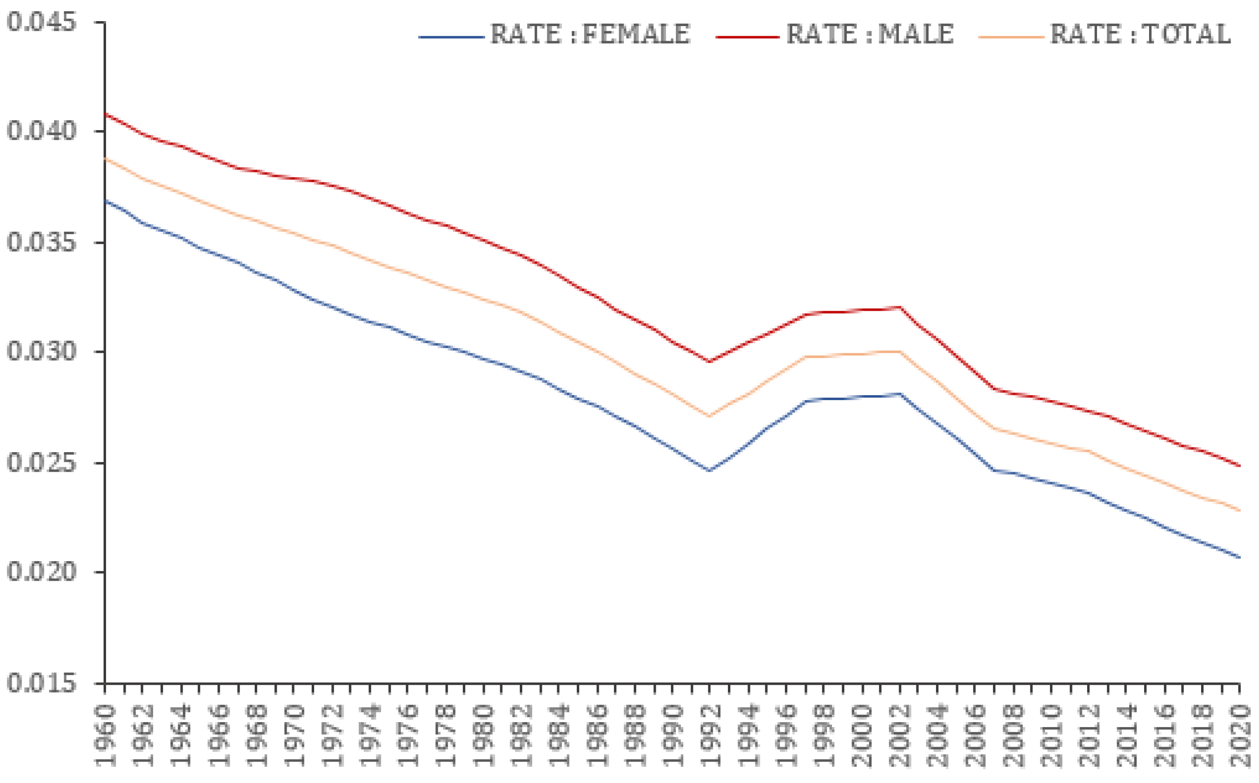
From Figure 1, mortality from the last two decades shows more pronounced decline rates. Additionally, 
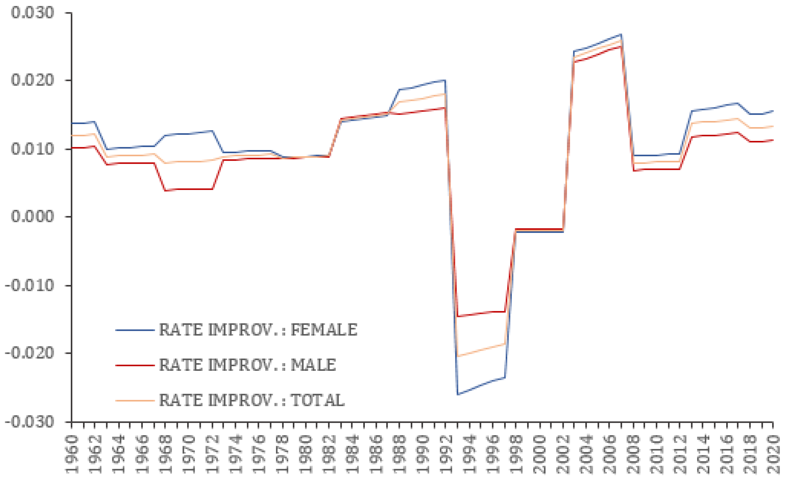
Figure 2 shows the mortality improvement (i.e., female, male, and total) that has been witnessed in the Ghana adult population since 1960. It is observed that the rate of improvement has been positive over the years. Although the rate improvement has no discernible pattern other than increasing on average, the last ten years have shown positively increasing mortality rates. Furthermore, the desriptive statistics (see Table 1) relating to female, male, and total population mortality improvement show that females have higher mortality improvement than males in Ghana (mean = 1.393% > 1.078%), with overall mortality improvement averaging 1.236% per year-on-year analysis. Half-decade mortality rates from the 2000s also showed that mortality rates have been improving for the population of both sexes but at decreasing rates.

3.3. Stochastic Mortality Models Estimation

Parameters of interest in the models ( k t ( 1 ) , k t ( 2 ) , γ t x ) show the rate improvement resulting from age-period and cohort group exposure over time. These are estimated using the R software and plotted to observe their shapes from the pensioners’ mortality data from 2010 to 2020 and within the ages of 40–83 years.

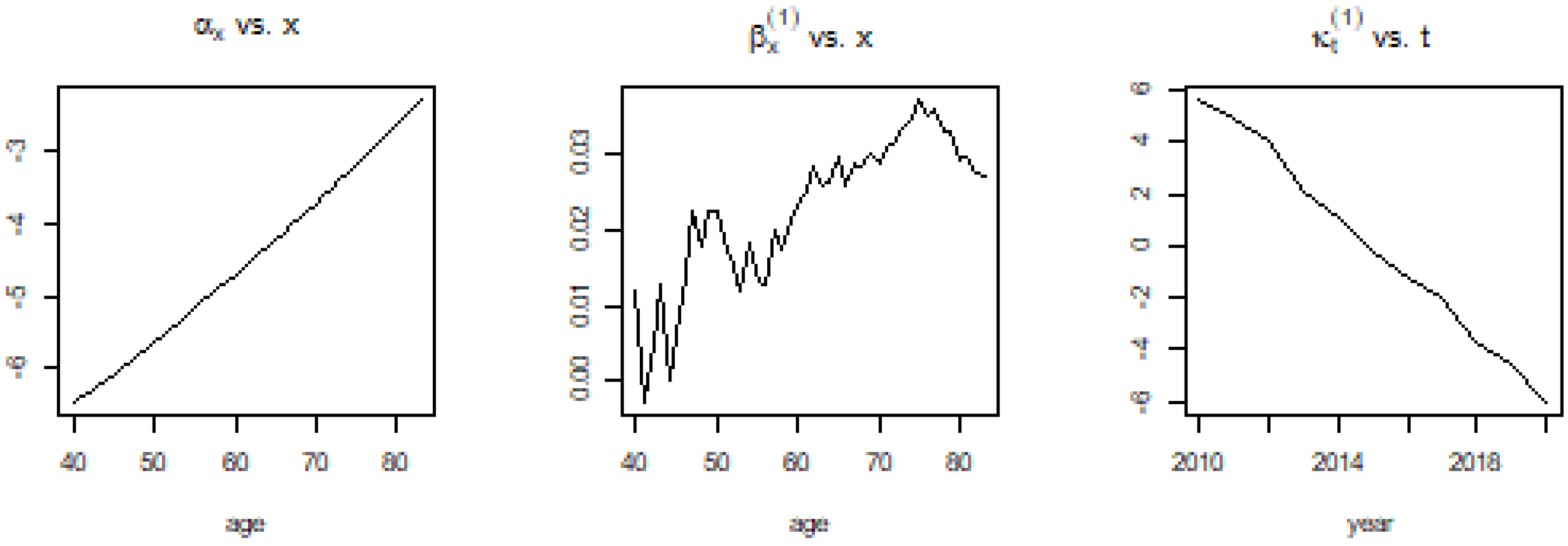
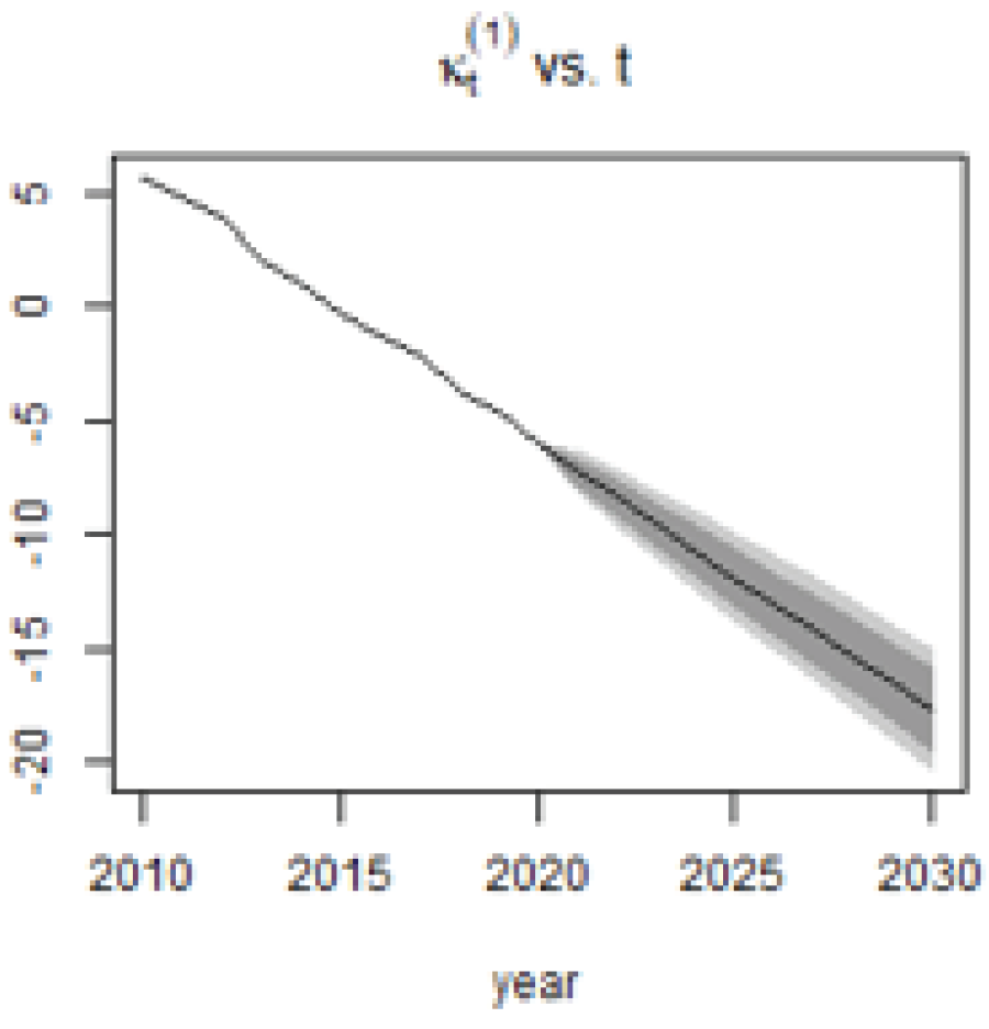
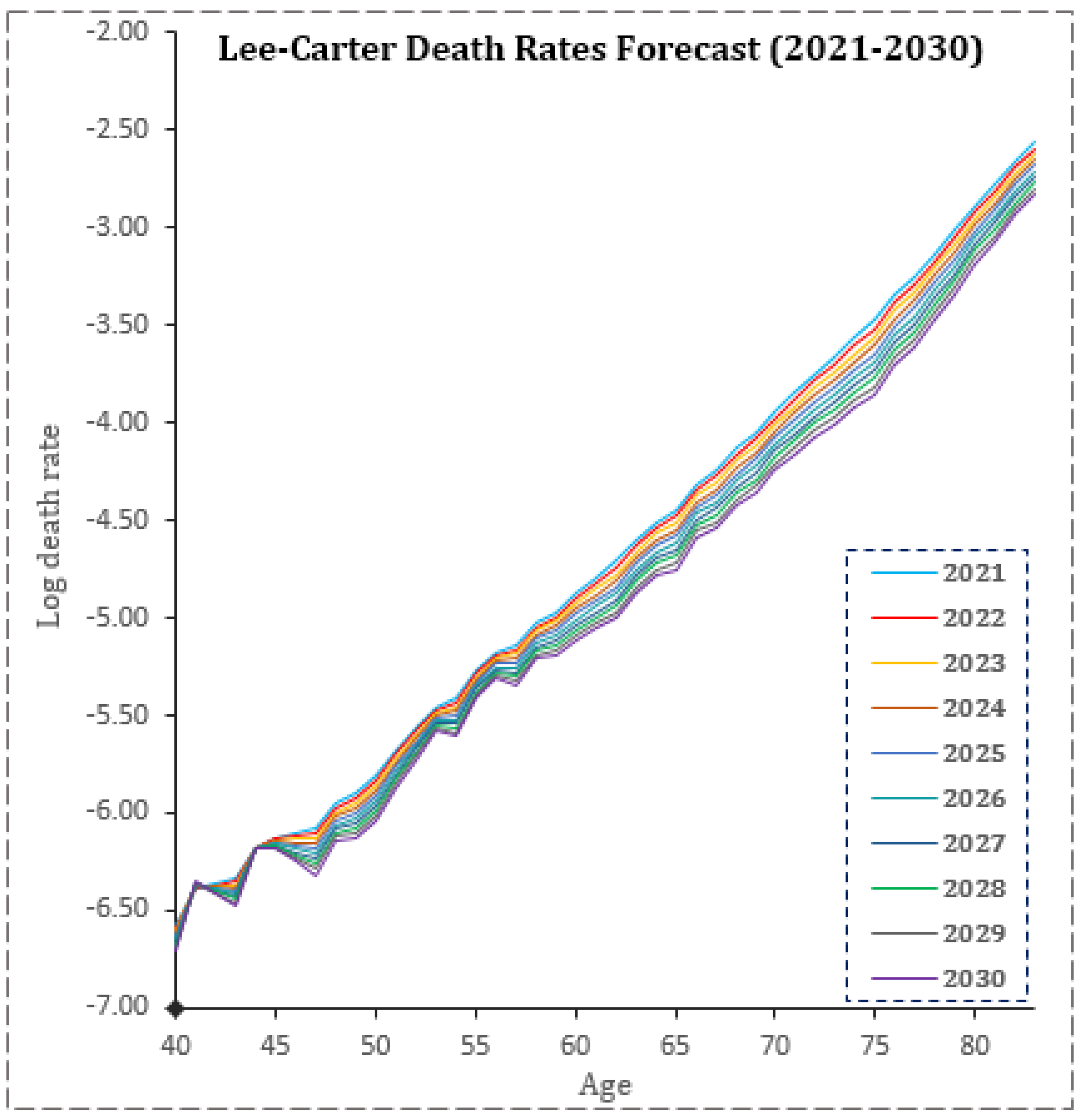
3.3.1. Lee-Carter Model

As shown in Figure 3, the overall rate of mortality improvement ( k t ( 1 ) ) is slowing, indicating that mortality has been declining for a long time. This is supported by the speed coefficient ( β x ( 1 ) ), which rises with increasing age. This, therefore, shows that the Lee–Carter model predicts decreasing mortality rates in the future.

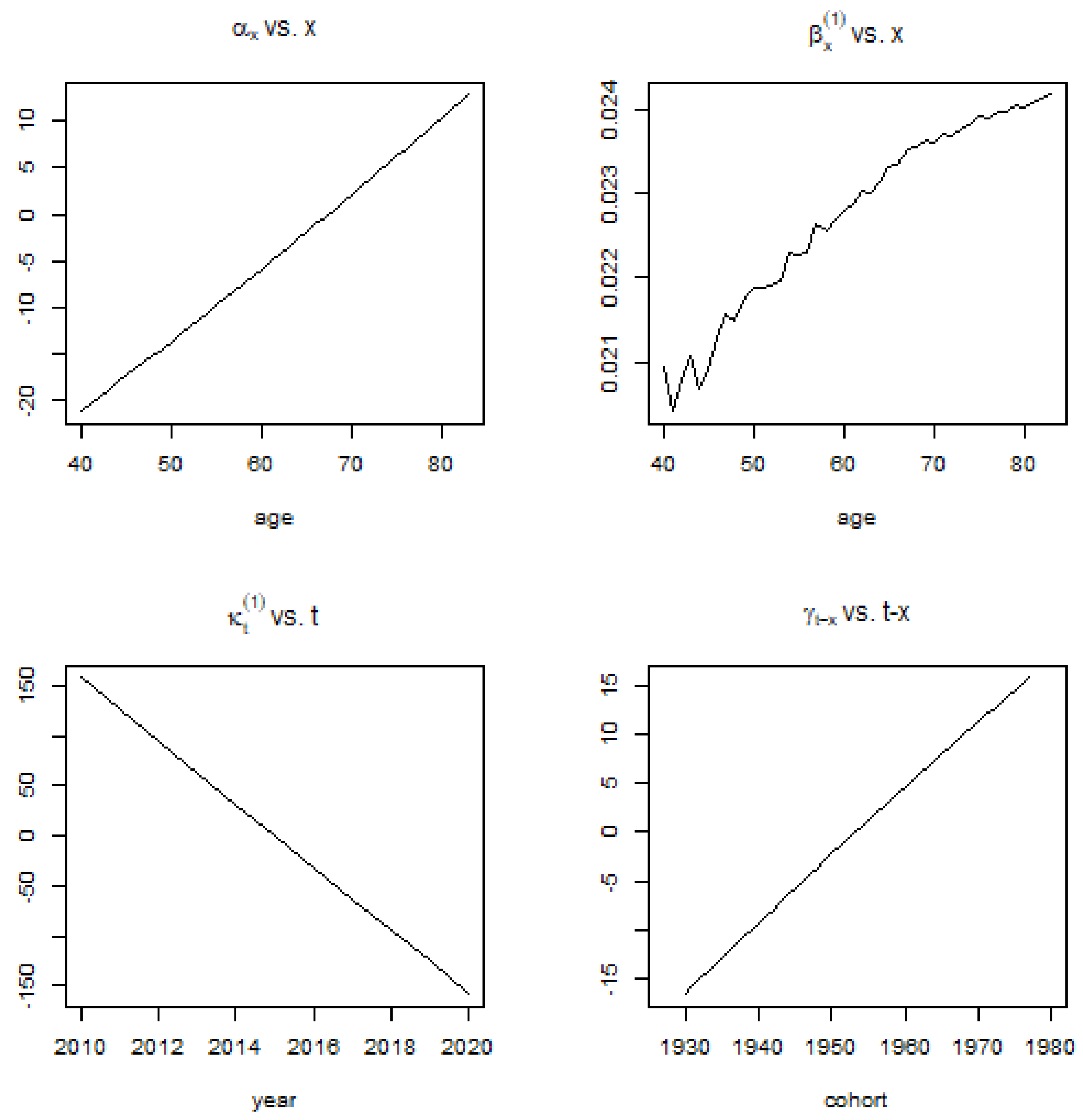
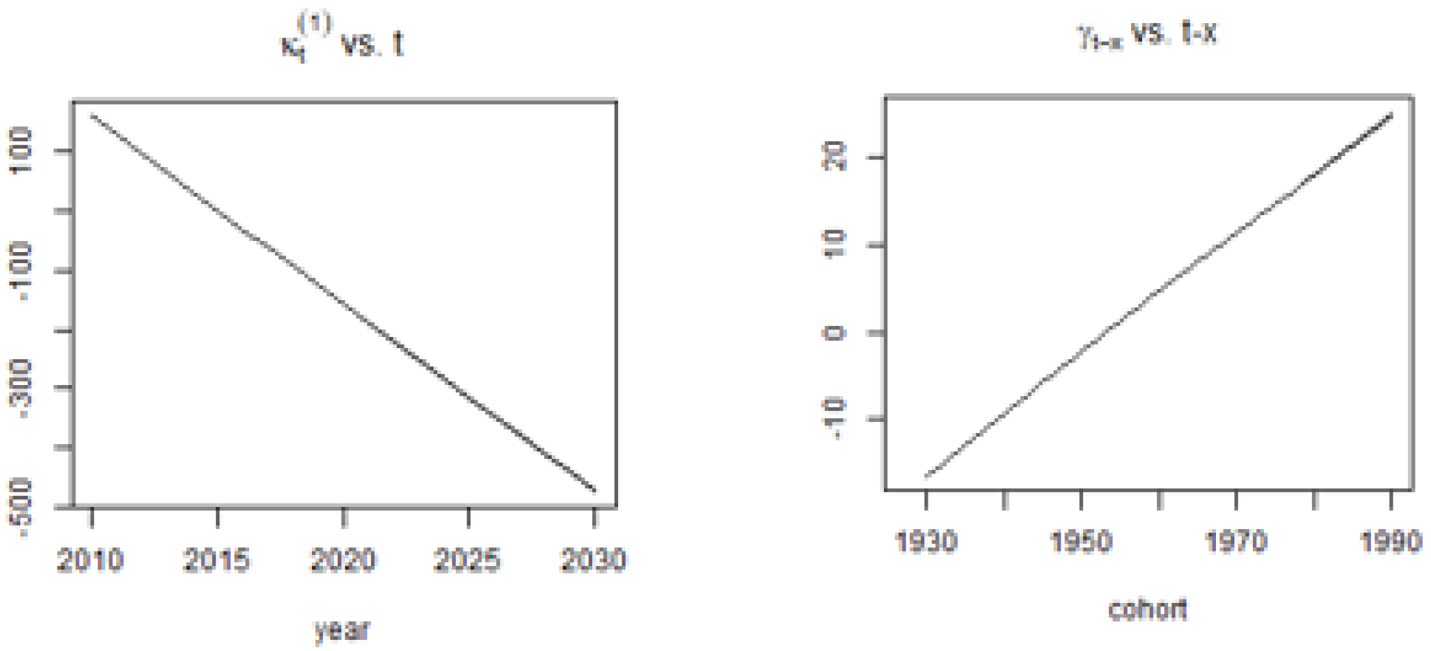
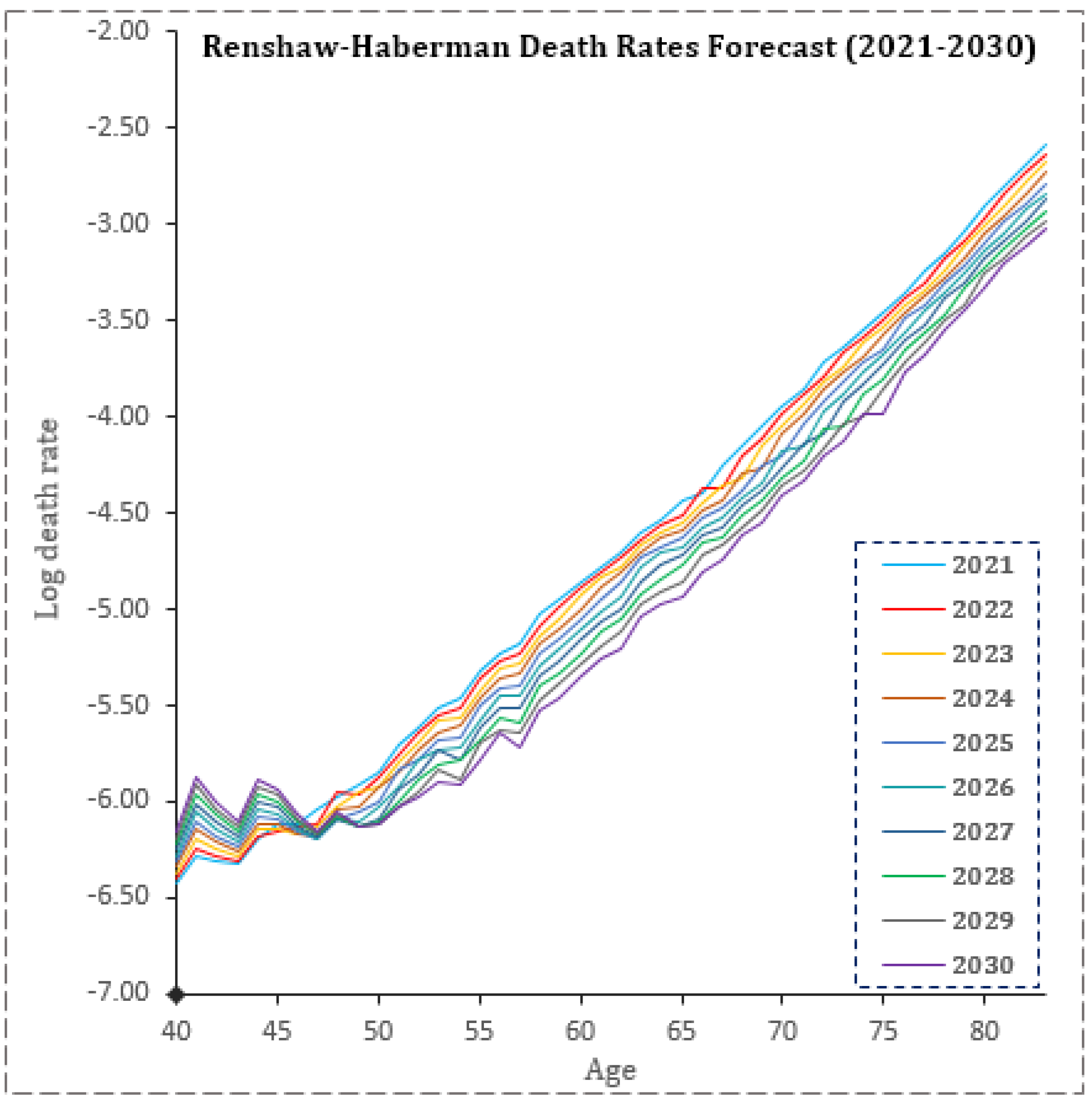
3.3.2. Renshaw–Haberman Model

Renshaw–Haberman’s model shows similar observations for the parameters ( k t ( 1 ) and β x ( 1 ) ) similar to the Lee–Carter model. This demonstrates that the cohort effect is increasing over time, and as such, cohorts in later years have higher mortality improvements. In Figure 4, the parameters of the Renshaw–Haberman Model is fitted to the Ghana Pension Population for Ages 40–83 and the Period 2010–2020.

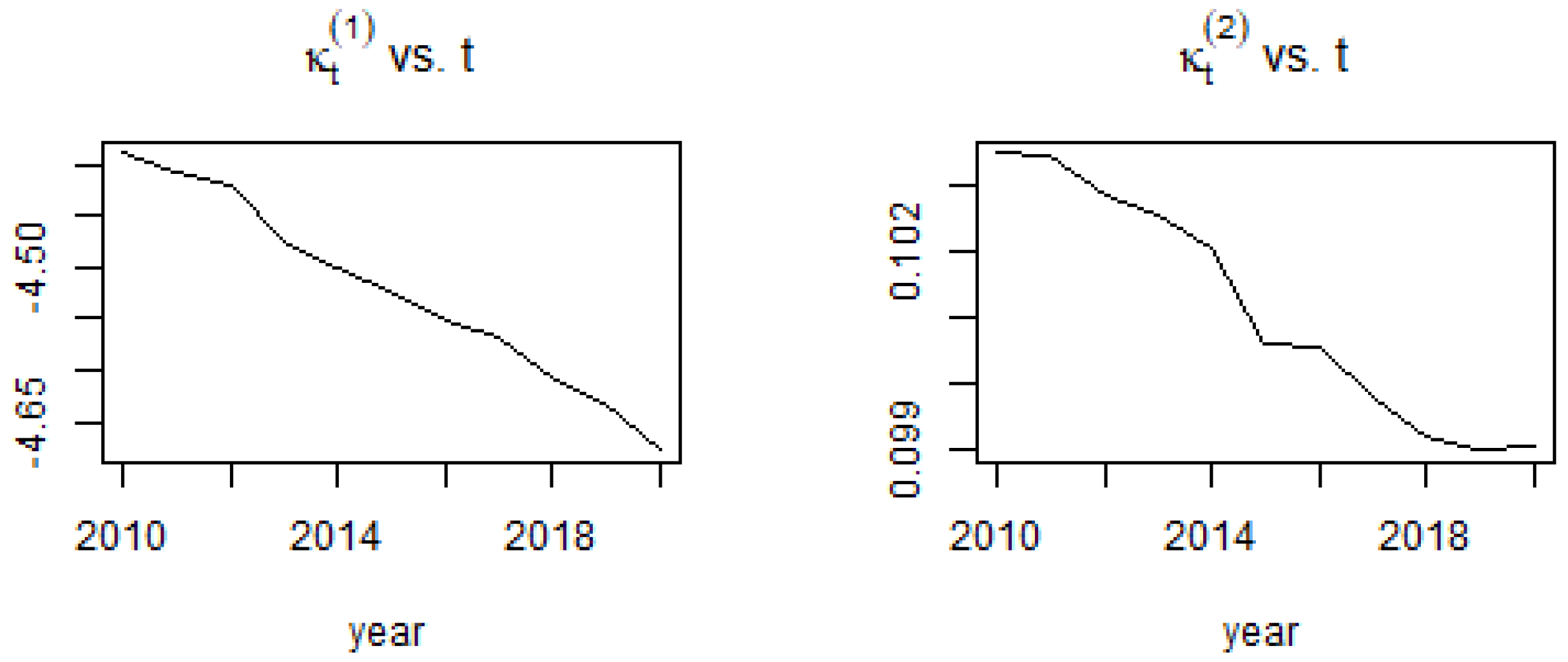
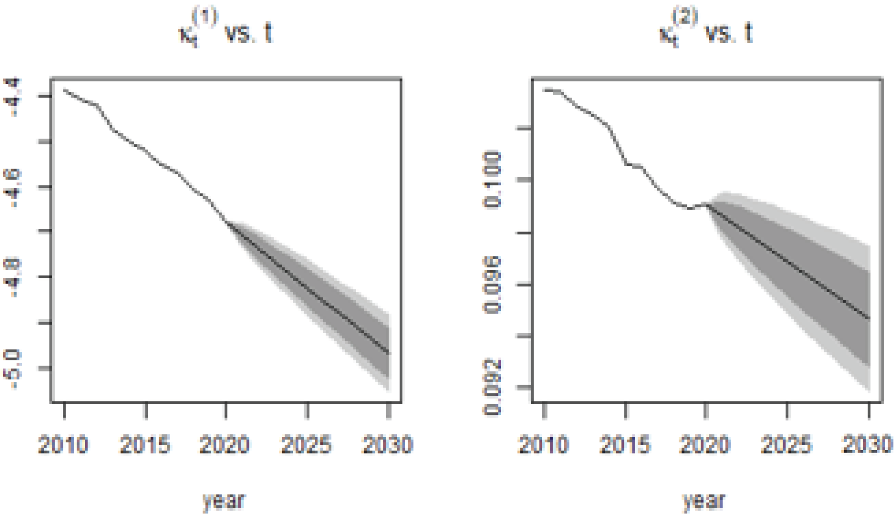
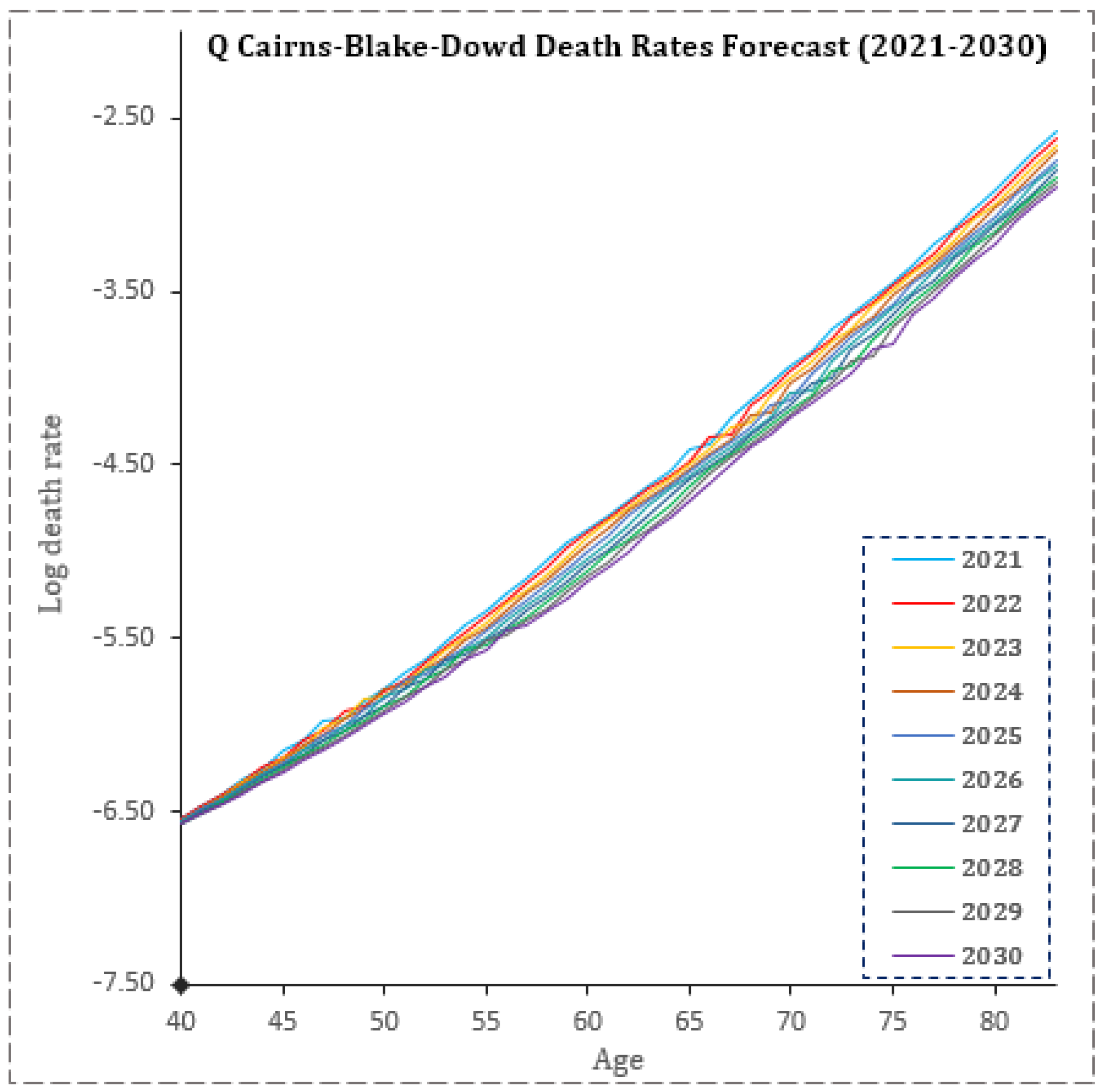
3.3.3. Cairns-Blake-Dowd Model

Cairns et al. model shows declining mortalities for both period effects ( k t ( 1 ) and k t ( 2 ) ) of the pensioners’ mortality data [26]. This is observed in Figure 5 below.

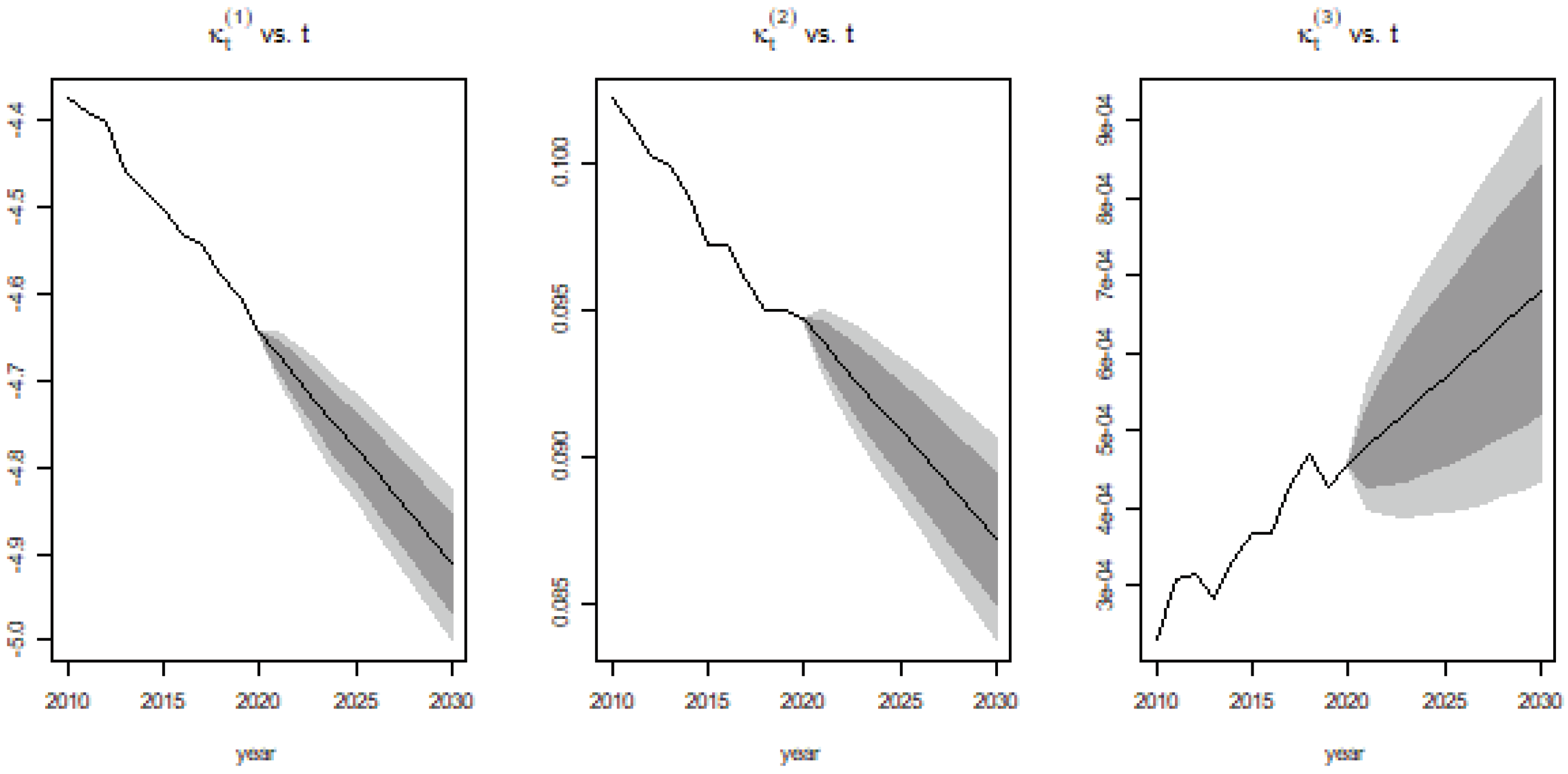
3.3.4. Quadratic Cairns–Blake–Dowd Model

Similarly, Cairns et al.’s quantitative extension of their original 2006 model shows declining period effects k t ( 1 ) and k t ( 2 ) , but the quadratic term rises over time [28]. This indicates that the average variation in mortality relating to period t is increasing (see Figure 6).

3.4. Models Goodness of Fit

The mortality models are subject to diagnostic and selection criteria to determine the most optimal fit to the pensioners’ mortality data in order to compute rate improvements. The MAFE, RMSSFE, and MAPFE are used in evaluating the mortality models. Table 2 demonstrates that the quadratic Cairns–Blake–Dowd model exhibits the best fit to the mortality data and has the lowest MAFE, RMSFE, and MAPFE. Moreover, the residual statistics in Figure 7, Figure 8, Figure 9 and Figure 10 give further evidence to support the model selection. While the Q-CBD shows greater fitness to the mortality data, all four models were used for forecasting to observe variations around forecasted mortality rates.
Using the Diebold–Mariano test [29], the predictive accuracy of the models are compared using the following hypotheses,
H 0 : Model 1 is not more accurate than Model 2.
H 1 : Model 1 is more accurate than Model 2.
Clearly, from Table 3, Q-CBD = LC > CBD > RH. This is consistent with the results obtained from Table 2.
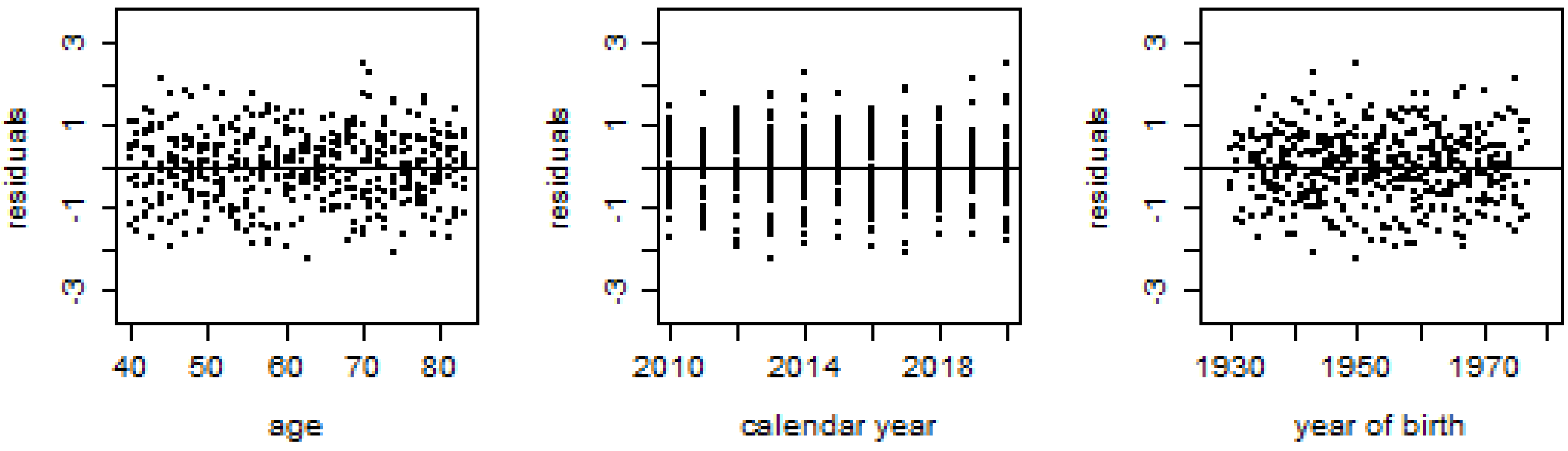
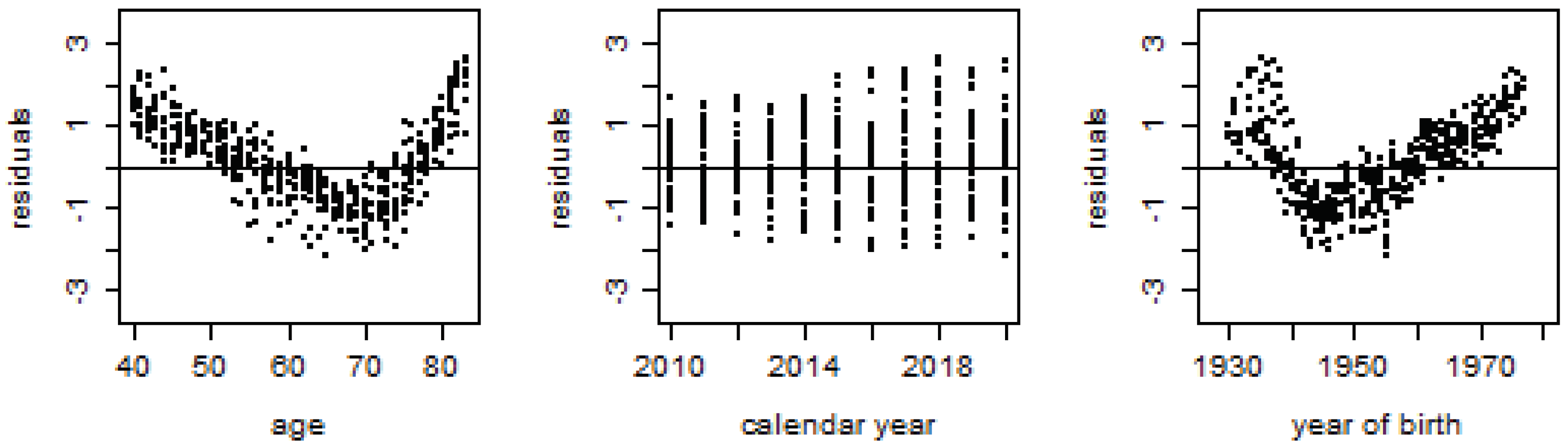
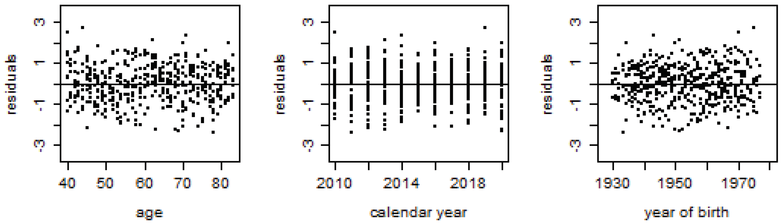
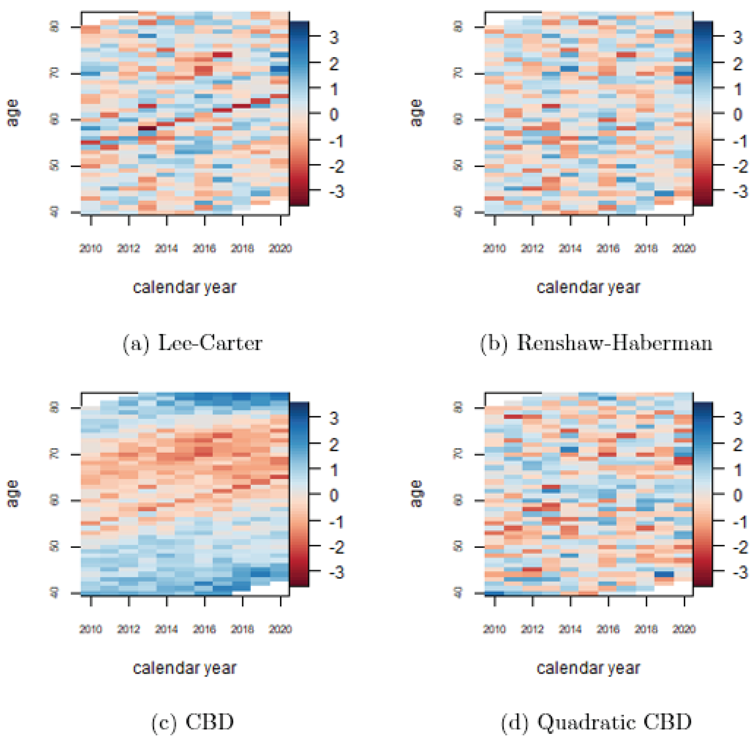
The residual plots in Figure 7, Figure 8, Figure 9 and Figure 10 show that almost all the models fit the mortality data well except the CBD model (Figure 9), which shows the age and cohort effects will be appropriately modeled by some quadratic function (Q-CBD). This is further reflected in the heat-map snippet (c) in Figure 11. This map shows a reduced amount of roughness, thus indicating a low level of randomness in residuals as compared to the LC, RH, and Q-CBD heat maps.

3.5. Mortality Models Rate Forecasts

From 2021 to 2030, model parameters were predicted to follow discernible paths. As seen in Figure 12, Figure 13, Figure 14 and Figure 15, all models show period and cohort effects to be, respectively, decreasing and increasing within the forecasting horizon. These models are then used to produce the rates forecast for the calendar years 2021–2030 (see Appendix A).

3.6. Mortality Improvement

Mortality improvements associated with the four models are shown in Table 4. The greatest risk to pension funds is from those of pensionable age who live beyond their expected lifespan. Observations from the forecasted improvement rates for pension ages 60, 65, 70, 75, and 80 show no major discernible differences between the values produced by the models. The Renshaw–Haberman model also produced the largest estimates of mortality improvement within two, five, and ten years. Additionally, the models produced increasing mortality improvements for increasing ages in the retirement frame. This should let the people who run pension plans know that their pensioners may have a higher chance of living longer than the general population. Furthermore, relying on the Q-CBD, the overall mortality improvement for ages 40–83 expected within 2021–2030 is around 2.534% (see Table 4), which is double the national average of 1.236% (see Table 1). This should inform pension plan sponsors that their pension participants may have a higher mortality improvement than the general population.

3.7. Present Annuity Value Factor for Pension Ages

The projected annuity value factor within 2021–2030 for ages 55, 57, 60, 62, and 65 is summarized in Table 5, Table 6, Table 7 and Table 8 for the four models. The GHS 1 annual pension cost paid GHS 1/12 monthly for pensionable ages shows no strong differences in the single annuity value for the ages 55, 57, 60, 62, and 65. This demonstrates that as members age, their mortality rate decreases, having no effect on pension costs as a result of the improved mortality rate. This is observed in Table 5, Table 6, Table 7 and Table 8, where the annuities for all models show no differences in value with increasing ages. In other words, the amount expected to be paid to a 55-year-old is the same as the amount expected to be paid to a 65-year-old within the pension period.

3.8. Discussion

As seen, the time-varying effects of age, period, and cohort are fittingly modeled by the quadrature CBD due to the curvature of age and cohort (birth year). Often, this model is an improvement over the Lee–Carter and the CBD base models, especially when curvature in age, period, or dimensional cohort effects are observed in mortality data, as seen in this study. The actuarial profession has acknowledged the fitting importance of such curve inclusion in U.S., UK, and Canadian mortality models, as well as other countries, and this has proved significantly important for pension managers in pension ratemaking [30,31,32,33]. The study’s identification of the Cairns–Blake–Dowd model with quadratic age and cohort effects for the Ghanaian pensioners’ mortality is significant in estimating mortality improvement for pensionable ages. Furthermore, all models revealed a decreasing mortality trend (increasing longevity improvement) among aging pensioners. This is in tandem with numerous studies, including [31,32,34], who found that pensioners in current times live longer than anticipated and that the effects of age and cohort are hugely evident. Resulting from the decreasing nature of mortality for the pensioners, the longevity risk, as measured by the mortality improvement, was severe. This indicated that older ages are associated with greater improvements than expected, while similar observations are made in several countries, even in gender disparity models [35]. However, a decreasing life expectancy was seen in Malaysia among pensioners and among the aging population [36,37].
Moreover, anticipated increases in expectancy increase the projected annuities for pensions. This study showed increasing annuities for pensioners within the pensionable age range. Furthermore, the improvement compensates for the effect of aging within the pensionable age or the retirement period. This is also in line with what has been seen in the literature, where the amount paid to annuitants increases with age due to the direct relationship between annuities and mortality improvements [38,39].
Furthermore, longevity risk as measured by the mortality improvement in this study showed that older ages were associated with greater mortality improvement, which was, on average, about 2.534% in the study’s forecasted horizon (2021–2030). This was more than the national mortality average of 1.236%. Furthermore, the projected annuity value within the study’s horizon showed no significant differences in value for pension ages 55, 57, 60, 62 and 65 years, thus indicating that the improvement seems to diminish the effect of increasing age within the retirement period.

4. Conclusions and Policy Recommendation

In this paper, we estimate the longevity risk associated with Ghana’s pension scheme and determine its possible impact on the sponsor’s liability over time. Using different stochastic mortality models (Lee–Carter, Renshaw–Haberman, Cairns–Blake–Dowd, and Quadratic Cairns–Blake–Dowd), we forecast the mortality improvements between 2021 and 2030. In the analysis, the Lee–Carter, Renshaw–Haberman, and Cairns–Blake–Dowd models predicted a decreasing trend in mortality rate for pensioners. This meant that pensioners’ ages did not seem to predict an increasing mortality rate as expected, and all mortality improvement parameters were trending downward within the study’s forecasted horizon (2021–2030). Owing to this, the forecasted mortality rates for pension participants are expected to decrease further, resulting in serious longevity risk for the pension scheme in the next ten years. The longevity risk, as measured by the mortality improvement, showed that older ages are associated with greater mortality improvement, which averages about 2.534% in the study’s forecasted horizon (2021–2030). This is more than the national mortality average of 1.236%. Hence, in the next ten years, the notion of older people dying faster among the pension participants may be diminished since, even at such ages, participants have greater chances of surviving the next period than even those who are young. Furthermore, the projected annuity value within the study’s horizon showed no significant differences in value for pension ages of 55, 57, 60, 62, and 65 years, indicating that the improvement seems to diminish the effect of increasing ages within the retirement period. Owing to these observations, the impact on the scheme was direct. The present annuity value showed that the monies that are expected to be paid to pensioners who have already received about five years of pension are no different from those who just went on the pension. This shows the canceling effect of longevity on ages within the retirement period.
Based on the conclusion, it is recommended that pension plan sponsors in Ghana look to explore longevity-bearing assets to tackle the effect of the longevity improvement observed among pension participants. This should seek to immunize the canceling effect of mortality improvement associated with increasing ages within the retirement period. Furthermore, other than general longevity risks that affect pension schemes, there exist different risk features such as socioeconomic associations [40] and asymmetry in mortality [41] that also affect the scheme. In future studies, we will extend this paper to include these other risk features. Future studies will also compare the stochastic mortality models used in this paper to Bayesian formalization, such as that contained in the paper of Giudici et al. [42].

Author Contributions

Conceptualization, S.A.G.; Methodology, J.A., S.W.A. and Y.S.; Software, Y.S.; Validation, S.A.G.; Formal analysis, J.A., S.W.A. and Y.S.; Investigation, Y.S.; Data curation, J.A.; Writing—original draft, S.W.A. and J.A.; Writing—review and editing, S.A.G.; Supervision, S.A.G.; Project administration, S.A.G. All authors have read and agreed to the published version of the manuscript.

Funding

This work did not receive any funding.

Institutional Review Board Statement

Not Applicable.

Informed Consent Statement

Not Applicable.

Data Availability Statement

Data are available from the corresponding author upon request.

Acknowledgments

The authors wish to thank the academic editor and anonymous referees for their comments.

Conflicts of Interest

The authors declare that they have no known competing financial interests or personal relationships that could have appeared to influence the work reported in this paper.

Appendix A. Mortality Rate Forecasts—Pension Ghana

Figure A1. Lee–Carter Rate Forecast for Period 2021–2030.
Fintech 02 00004 g0a1
Figure A2. Renshaw–Haberman Rate Forecast for Period 2021–2030.
Fintech 02 00004 g0a2
Figure A3. Cairns–Blake–Dowd Rate Forecast for Period 2021–2030.
Fintech 02 00004 g0a3
Figure A4. Quadratic Cairns–Blake–Dowd Rate Forecast for Period 2021–2030.
Fintech 02 00004 g0a4

References

  1. United States Central Intelligence Agency; United States Government Publications Office. The World Factbook 2014-15; Government Printing Office: Washington, DC, USA, 2015. [Google Scholar]
  2. World Bank. Life Expectancy at Birth, Total (Years). 2021. Available online: https://data.worldbank.org/indicator/SP.DYN.LE00.IN (accessed on 23 October 2022).
  3. Hari, N.; De Waegenaere, A.; Melenberg, B.; Nijman, T.E. Longevity risk in portfolios of pension annuities. Insur. Math. Econ. 2008, 42, 505–519. [Google Scholar] [CrossRef]
  4. Richards, S.J.; Jones, G.L. Financial Aspects of Longevity Risk; Prudential Assurance Company: London, UK, 2004. [Google Scholar]
  5. De Waegenaere, A.; Melenberg, B.; Stevens, R. Longevity risk. Economist 2010, 158, 151–192. [Google Scholar] [CrossRef]
  6. Kurtbegu, E. Replicating intergenerational longevity risk sharing in collective defined contribution pension plans using financial markets. Insur. Math. Econ. 2018, 78, 286–300. [Google Scholar] [CrossRef]
  7. Agarwal, A.; Ewald, C.O.; Wang, Y. Hedging longevity risk in defined contribution pension schemes. arXiv 2019, arXiv:1904.10229. [Google Scholar] [CrossRef] [Green Version]
  8. Antolin, P. Longevity Risk and Private Pensions OECD Working Papers on Insurance and Private Pensions No. 3; OECD Publishing: Paris, France, 2007. [Google Scholar]
  9. Ofori-Amanfo, E.K. Forecasting Mortality Rates and Modelling Longevity Risk of SSNIT Pensioners. Ph.D. Thesis, University of Ghana, Accra, Ghana, 2019. [Google Scholar]
  10. Kessler, A. New solutions to an age-old problem: Innovative strategies for managing pension and longevity risk. N. Am. Actuar. J. 2021, 25, S7–S24. [Google Scholar] [CrossRef] [Green Version]
  11. Kalu, G.O.; Ikpe, C.D.; Oruh, B.I.; Gyamerah, S.A. State Space Vasicek Model of a Longevity Bond. arXiv 2020, arXiv:2011.12753. [Google Scholar]
  12. Assabil, S.E.; McLeish, D.L. Assessing the Impact of Longevity Risk for Countries with Limited Data. J. Retire. 2021, 8, 62–75. [Google Scholar] [CrossRef]
  13. Kimondo, W. Longevity Risk and Private Pension Funds-Analysis of Longevity Risk Using the Renshaw-haberman Model. Ph.D. Thesis, University of Nairobi, Nairobi, Kenya, 2018. [Google Scholar]
  14. Adegbilero-Iwari, O.E.; Chukwu, A.U. Modelling Nigerian Female Mortality: An Application of Four Stochastic Mortality Models. In Quantitative Methods in Demography; Springer: Cham, Switzerland, 2022; pp. 229–244. [Google Scholar]
  15. Nantwi, N.P.A.; Lotsi, A.; Debrah, G. Longevity risk–Its financial impact on pensions. Sci. Afr. 2022, 16, e01241. [Google Scholar] [CrossRef]
  16. Odhiambo, J.; Ngare, P.; Weke, P. Bühlmann credibility approach to systematic mortality risk modeling for sub-Saharan Africa populations (Kenya). Res. Math. 2022, 9, 2023979. [Google Scholar] [CrossRef]
  17. Adebowale, A.S.; Fagbamigbe, A.F.; Olowolafe, T.; Afolabi, R.F. Dynamics of Adult Mortality in Sub-Saharan Africa: Are there prospects for decline. In The Routledge Handbook of African Demography; Routledge: Oxfordshire, UK, 2022; pp. 745–768. [Google Scholar]
  18. Lee, R.D.; Carter, L.R. Modeling and forecasting US mortality. J. Am. Stat. Assoc. 1992, 87, 659–671. [Google Scholar]
  19. Cairns, A.J.; Blake, D.; Dowd, K. Modelling and management of mortality risk: A review. Scand. Actuar. J. 2008, 2008, 79–113. [Google Scholar] [CrossRef]
  20. Cairns, A.J. Robust hedging of longevity risk. J. Risk Insur. 2013, 80, 621–648. [Google Scholar] [CrossRef]
  21. Bisetti, E.; Favero, C.A. Measuring the impact of longevity risk on pension systems: The case of Italy. N. Am. Actuar. J. 2014, 18, 87–103. [Google Scholar] [CrossRef]
  22. Blake, D.; Cairns, A.J. Longevity risk and capital markets: The 2018–19 update. Ann. Actuar. Sci. 2020, 14, 219–261. [Google Scholar] [CrossRef]
  23. Broeders, D.; Mehlkopf, R.; van Ool, A. The economics of sharing macro-longevity risk. Insur. Math. Econ. 2021, 99, 440–458. [Google Scholar] [CrossRef]
  24. Levantesi, S.; Nigri, A.; Piscopo, G. Improving longevity risk management through machine learning. In The Essentials of Machine Learning in Finance and Accounting; Routledge: Oxfordshire, UK, 2021; pp. 37–56. [Google Scholar]
  25. Renshaw, A.E.; Haberman, S. A cohort-based extension to the Lee–Carter model for mortality reduction factors. Insur. Math. Econ. 2006, 38, 556–570. [Google Scholar] [CrossRef]
  26. Cairns, A.J.; Blake, D.; Dowd, K. A two-factor model for stochastic mortality with parameter uncertainty: Theory and calibration. J. Risk Insur. 2006, 73, 687–718. [Google Scholar] [CrossRef]
  27. Currie, I.D. On fitting generalized linear and non-linear models of mortality. Scand. Actuar. J. 2016, 2016, 356–383. [Google Scholar] [CrossRef]
  28. Cairns, A.J.; Blake, D.; Dowd, K.; Coughlan, G.D.; Epstein, D.; Ong, A.; Balevich, I. A quantitative comparison of stochastic mortality models using data from England and Wales and the United States. N. Am. Actuar. J. 2009, 13, 1–35. [Google Scholar] [CrossRef]
  29. Diebold, F.; Mariano, R. Comparing predictive accuracy. J. Bus. Econ. Stat. 1995, 13, 253–263. [Google Scholar]
  30. Li, J.S.H.; Liu, Y. Constructing Two-Dimensional Mortality Improvement Scales for Canadian Pension Plans and Insurers: A Stochastic Modelling Approach; Canadian Institute of Actuarie: Ottawa, ON, Canada, 2019. [Google Scholar]
  31. Wen, J.; Kleinow, T.; Cairns, A.J. Trends in canadian mortality by pension level: Evidence from the CPP and QPP. N. Am. Actuar. J. 2020, 24, 533–561. [Google Scholar] [CrossRef]
  32. Yildirim, İ. Longevity Risk and Modelling in The Life and Pension Insurance Company. İstatistikçiler Dergisi: İstatistik Ve Aktüerya 2021, 14, 30–43. [Google Scholar]
  33. Ayuso, M.; Bravo, J.M.; Holzmann, R. Getting life expectancy estimates right for pension policy: Period versus cohort approach. J. Pension Econ. Financ. 2021, 20, 212–231. [Google Scholar] [CrossRef]
  34. Pérez-Salamero González, J.M.; Regúlez-Castillo, M.; Ventura-Marco, M.; Vidal-Meliá, C. Mortality and life expectancy trends in Spain by pension income level for male pensioners in the general regime retiring at the statutory age, 2005–2018. Int. J. Equity Health 2022, 21, 1–21. [Google Scholar] [CrossRef] [PubMed]
  35. Pérez Salamero González, J.M.; Regúlez-Castillo, M.; Vidal-Meliá, C. Mortality and life expectancy trends for male pensioners by pension income level. SSRN 2021. [Google Scholar] [CrossRef]
  36. Zulkifle, H.; Yusof, F.; Nor, S.R.M. Comparison of Lee Carter model and Cairns, Blake and Dowd model in forecasting Malaysian higher age mortality. Mat. Malays. J. Ind. Appl. Math. 2019, 35, 65–77. [Google Scholar] [CrossRef]
  37. Ibrahim, R.I.; Nordin, N.M. Analysis of mortality improvement on the pension cost due to aging population. Mat. Malays. J. Ind. Appl. Math. 2020, 6, 209–216. [Google Scholar] [CrossRef]
  38. Richman, R.; Velcich, G. Mortality Improvements in South Africa: Insights from Pensioner Mortality. 2020. Available online: https://ssrn.com/abstract=3688919 (accessed on 23 October 2022).
  39. Chang, C.K.; Yue, J.C.; Chen, C.J.; Chen, Y.W. Mortality differential and social insurance: A case study in Taiwan. N. Am. Actuar. J. 2021, 25, S582–S592. [Google Scholar] [CrossRef]
  40. Lyu, P.; Li, J.S.H.; Zhou, K.Q. Socioeconomic differentials in mortality: Implications on index-based longevity hedges. Scand. Actuar. J. 2022, 1–29. [Google Scholar] [CrossRef]
  41. Zhou, K.Q.; Li, J.S.H. Asymmetry in mortality volatility and its implications on index-based longevity hedging. Ann. Actuar. Sci. 2020, 14, 278–301. [Google Scholar] [CrossRef]
  42. Giudici, P.; Mezzetti, M.; Muliere, P. Mixtures of products of Dirichlet processes for variable selection in survival analysis. J. Stat. Plan. Inference 2003, 111, 101–115. [Google Scholar] [CrossRef]
Figure 1. Mortality Rates per 1000 Adult Population 1960–2020.
Fintech 02 00004 g001
Figure 2. Rates Improvement per 1000 Adult Population 1960–2020.
Fintech 02 00004 g002
Figure 3. Lee–Carter Parameters Fitted to the Ghana Pension Population for Ages 40–83 and the Period 2010–2020.
Fintech 02 00004 g003
Figure 4. Renshaw–Haberman Parameters fitted to the Ghana Pension Population for Ages 40–83 and the Period 2010–2020.
Fintech 02 00004 g004
Figure 5. CBD Parameters Fitted to the Ghana Pension Population for Ages 40–83 and the Period 2010–2020.
Fintech 02 00004 g005
Figure 6. Quadratic CBD parameters Fitted to the Ghana Pension Population for Ages 40–83 and the Period 2010–2020.
Fintech 02 00004 g006
Figure 7. LC Deviance Residuals from the Fitted Model to the Ghana Pension Population for Ages 40–84 and the Period 2010–2020.
Fintech 02 00004 g007
Figure 8. RH Deviance Residuals from the Fitted Model to the Ghana Pension Population for Ages 40–83 and the Period 2010–2020.
Fintech 02 00004 g008
Figure 9. CBD Deviance Residuals from the Fitted Model to the Ghana Pension Population for Ages 40–83 and the Period 2010–2020.
Fintech 02 00004 g009
Figure 10. Q-CBD Deviance Residuals from the Fitted Model to the Ghana Pension Population for Ages 40–83 and the Period 2010–2020.
Fintech 02 00004 g010
Figure 11. Heat Map of Deviance Residuals for Models.
Fintech 02 00004 g011
Figure 12. Parameter Forecast using the Lee–Carter Model.
Fintech 02 00004 g012
Figure 13. Parameter Forecast using the Cairns–Blake–Dowd model.
Fintech 02 00004 g013
Figure 14. Parameter Forecast using the Renshaw–Haberman Model.
Fintech 02 00004 g014
Figure 15. Parameter Forecast using the Quadratic Cairns–Blake–Dowd Model.
Fintech 02 00004 g015
Table 1. Descriptive Statistics on Mortality Improvement in the Ghanaian Population (1960–2020).
FemaleMaleTotal
Moment Measure(%)(%)(%)
Mean1.3931.0781.236
Median1.3220.9601.066
Standard deviation0.6500.5650.588
Half-Decades Rate Improvement
2001–20051.5801.4711.525
2006–20101.6041.4061.505
2011–20151.3220.9981.160
2016–20201.5741.1631.368
Table 2. Accuracy Assessment for Model Selection.
MetricLCRHCBDQ-CBD
MAFE 4.2 × 10 3 1.0 × 10 2 1.3 × 10 2 3.9 × 10 3
RMSFE 7.4 × 10 3 2.0 × 10 2 2.2 × 10 2 5.8 × 10 3
MAPFE3.4%6.7%7.6%2.9%
Rank(2)(3)(4)(1)
Table 3. Diebold–Mariano (DM) Test for Predictive Accuracy.
Model 1Model 2DM Statisticsp-Value
Q-CBDLC1.21500.8878
Q-CBDRH−2.99510.0014 **
Q-CBDCBD−1.95940.0250 **
LCRH−2.80880.0025 **
LCCBD−1.90070.0287 **
LCQ-CBD−1.21500.1122
RHCBD−1.43700.0754 *
* and ** represents the significance level at 10% and 5% respectively.
Table 4. Forecasted Mortality Improvement in 2, 5 and 10 Years from 2020 within Pension Ages.
Lee-Carter2021–20222021–20252021–2030
602.6512.6522.653
653.3383.3403.342
703.2613.2643.267
754.1164.1234.132
803.1953.2033.214
Overall: 40–802.575
Renshaw-Haberman
603.2234.7055.253
655.4604.7115.350
704.9624.6245.039
753.7004.2125.529
804.9574.4774.582
Overall: 40–804.256
CBD
602.7712.7722.773
652.9702.9722.974
703.1583.1613.165
753.3273.3323.339
803.4653.4743.486
Overall: 40–802.805
Quadratic CBD
602.0733.3213.217
654.3273.1313.316
703.7233.0933.261
752.6562.9743.875
804.1763.5883.456
Overall: 40–802.534
Table 5. Projected Annuity Factor Cost for Retirement Age—LC Estimates.
Age2021–20302021–2030
(Annually)(Monthly)
555.41915.8775
575.38545.8438
605.32375.7820
625.27485.7332
655.20095.6593
Table 6. Projected Annuity Factor Cost for Retirement Age—RH Estimates.
Age2021–20302021–2030
(Annually)(Monthly)
555.43145.8897
575.39885.8571
605.33145.7897
625.27975.7381
655.20755.6658
Table 7. Projected Annuity Factor Cost for Retirement Age—CBD Estimates.
Age2021–20302021–2030
(Annually)(Monthly)
555.42475.8830
575.38595.8443
605.32205.7803
625.26765.7260
655.18825.6465
Table 8. Projected Annuity Factor Cost for Retirement Age—Q-CBD Estimates.
Age2021–20302021–2030
(Annually)(Monthly)
555.42555.8838
575.38855.8468
605.32545.7838
625.27215.7304
655.19485.6532
Disclaimer/Publisher’s Note: The statements, opinions and data contained in all publications are solely those of the individual author(s) and contributor(s) and not of MDPI and/or the editor(s). MDPI and/or the editor(s) disclaim responsibility for any injury to people or property resulting from any ideas, methods, instructions or products referred to in the content.

