Equivalence Checking of System-Level and SPICE-Level Models of Linear Circuits ^†

Abstract

Due to the increasing complexity of analog circuits and their integration into System-on-Chips (SoC), the analog design and verification industry would greatly benefit from an expansion of system-level methodologies using SystemC AMS. These can provide a speed increase of over $\mathrm{100,000}$× in comparison to SPICE-level simulations and allow interoperability with digital tools at the system-level. However, a key barrier to the expansion of system-level tools for analog circuits is the lack of confidence in system-level models implemented in SystemC AMS. Functional equivalence of single Laplace Transfer Function (LTF) system-level models to respective SPICE-level models was successfully demonstrated recently. However, this is clearly not sufficient, as the complex systems comprise multiple LTF modules. In this article, we go beyond single LTF models, i.e., we develop a novel graph-based methodology to formally check equivalence between complex system-level and SPICE-level representations of Single-Input Single-Output (SISO) linear analog circuits, such as High-Pass Filters (HPF). To achieve this, first, we introduce a canonical representation in the form of a Signal-Flow Graph (SFG), which is used to functionally map the two representations from separate modeling levels. This canonical representation consists of the input and output nodes and a single edge between them with an LTF as its weight. Second, we create an SFG representation with linear graph modeling for SPICE-level models, whereas for system-level models we extract an SFG from the behavioral description. We then transform the SFG representations into the canonical representation by utilizing three graph manipulation techniques, namely node removal, parallel edge unification, and reflexive edge elimination. This allows us to establish functional equivalence between complex system-level models and SPICE-level models. We demonstrate the applicability of the proposed methodology by successfully applying it to complex circuits.

1. Introduction

The rising complexity of analog circuits and the ever-increasing system integration of analog and digital components have created a bottleneck for analog design verification. A major challenge in this regard is the simulation speed of SPICE-level models [1]. They often fail for large systems due to convergence related problems or are prohibitive in terms of computational time required. Traditionally, SPICE-level simulations [2] are used often with manual inspection of the results. These simulations, while slow, are still considered a golden standard and cannot be ignored. However, different levels of design abstractions and alternate representations (e.g., a behavioral model) of the circuit can be used to achieve significantly better simulation performance and earlier design verification of the Design Under Verification (DUV).

As a consequence, analog designs are moving towards a top-down approach. In this regard, Virtual Prototyping (VP) at the abstraction of Electronic System Level (ESL) is nowadays an established industrial practice [1,3,4,5,6]. The Timed Data Flow (TDF) Model of Computation (MoC) available in SystemC AMS offers a good trade-off between accuracy and simulation speed at the system level, and can provide a speed increase of over $\mathrm{100,000}$× [1] in comparison to SPICE-level simulations. TDF defines time domain processing, and is used to model the pure algorithmic or procedural description of the underlying design. In particular, TDF provides utilities to implement Laplace Transfer Functions (LTF) of linear systems. A transfer function model captures the frequency response of an analog circuit and provides a suitable platform for applying non-simulation/formal techniques to verify the circuit against its specification. Due to earlier availability and significantly faster simulation speed as opposed to SPICE-level simulations [1], the TDF models provide a design refinement methodology and enable early verification for analog/mixed-signal systems.

However, one of the main challenges in adopting SystemC AMS system-level models is the lack of equivalence checking methodologies for SystemC AMS and SPICE-level models. Equivalence checking proves the general functional equality of two implementations of a design. The implementations can be of different abstraction levels and different description methods such as transistor netlists and system-level languages. While equivalence checking methods are well established in the digital domain [7,8,9], analog circuit design flows are lacking formal or at least formalized verification methodologies [10,11,12,13,14,15,16,17,18]. When speaking about equivalence checking methodologies, we broadly consider approaches such as state-space coverage, model-checking, and reachability. Regardless of the specific approach, confidence in adopting SystemC AMS system-level analog models is low. As a consequence, completely relying on SystemC AMS system-level models becomes difficult. Due to the rising complexity of analog designs, this becomes a serious problem.

Contribution: In this article, we significantly extend the methods and applicability of our novel equivalence checking methodology from [19], which is, to the best of our knowledge, the first of its kind. Essentially, our approach operates directly on the system-level and SPICE-level models by combining the linear graph modeling technique with several graph operations to transform these complex models into a canonical representation. It is therefore a static method and not simulation-based. The canonical representation is used to overcome the main challenge, which is to show that the SPICE-level model is equivalent to the behavioral system-level model implemented in SystemC AMS. We leverage Signal-Flow Graphs (SFG) as an intermediate representation between the SPICE-level and the system-level model, which the canonical representation also relies on. In particular, the developed method extends the applicability of the method in [19] to the class of complex single-input single-output (SISO) linear analog circuits with passive and active components. Many analog circuits fall into the linear category, such as various classic electronic circuits and many analog filters. Some examples of supported circuits are analog High-Pass Filters (HPF), averager circuits, amplifiers operated in their linear region, linear computation circuits, etc., and their combinations. Additionally, the method is extended to handle more complex behavioral models with respect to the simple LTF models used in [19]. We demonstrate the applicability of the developed methodology by successfully applying it to complex linear analog circuits.

In summary, the main contributions of this paper are:

• A novel equivalence checking methodology for SPICE-level models and behavioral system-level models that go beyond single LTFs.
• Leverage SFGs, canonical representations, and linear graph modeling techniques.
• Extension of applicability to the complete class of complex SISO linear analog circuits.
• Demonstration of equivalence checking on complex filter models, Small-Signal Models (SSM), series connections, and linear analog computers.

2. Related Work

In their survey of equivalence checking, Zaki et al. [10] summarized the literature until 2007 and pointed out that all the presented methods employ a priori knowledge of the DUV in the development process. A further comparison of some equivalence checking methods was presented in [11] by Tarraf et al. along with the proposal of a new equivalence checking method based on reachability. It is observed in this work that the definition of the coverage measures is a difficult task and that many methods balance completeness against pessimism.

In their study of equivalence checking on the state-space, Hedrich and Barke [12] compared the vector fields of the systems on a point grid to check the equivalency of two different representations of circuits. The method is applicable to SISO circuits that can be described by a set of nonlinear time-invariant first-order differential equations. Ref.  [13] extended the method in [12] to circuits that are defined by differential-algebraic equations, [14] applied the method to new examples, and [15] generalized it to multi-input multi-output circuits. The equivalence checking method proposed in [12] is applicable to many circuits, but some important dynamics might be missed as the points on the grid are fixed distances apart on the canonical state space.

In an investigation into simulation-based equivalency checking, Singh and Li [16] developed mapping techniques for comparing signals in different domains and decreased the high computational burden of simulation-based approaches by developing techniques that reduce the input space. However, the method relies on typical system-level simulation stimuli, which cannot completely cover all behavior, and the authors highlight this point by calling their method semi-formal. Ain et al. [17] also worked on simulation-based equivalency and developed a systematic methodology with a focus on circuit features. However, no attempt was made to mitigate the possible incompleteness of the externally given test bench. The coverage issue of simulation-based verification was addressed by Saglamdemir et al. [18] through an optimization-based method for automatic generation of inputs. Unfortunately, a discussion on whether all essential input shapes can be represented with the given set of input parameters is missing. Another problem that was not addressed is the possibility of the optimization to return a local minimum.

A summary of the differences between these various works is given in

Table 1. A comparison of the related works.

Source	Approach	Verification Coverage	Applicable Circuits
[12,13,14,15]	State-space-based	Only at finite number of locations in the state-space	All
[16,17,18]	Simulation-based	Only for finite number of input signals	All
Proposed work	Structural analysis	Complete coverage	Only linear

. As seen in the table, a common deficiency of many methods in the existing literature is that they do not check equivalence with complete coverage of behavior. Therefore, even if these methods claim equivalence, the models might still behave differently in an overlooked gap. Our proposed equivalence checking methodology, which we introduced in [19], does not have this issue as the analysis and modification methods used, such as linear graph modeling and graph reduction, statically analyze the structure of the models. On the other hand, the applicability of the method was limited to linear analog filter circuits. Additionally, only behavioral models consisting of a single LTF were supported on the system-level side. The current paper extends this methodology such that it supports complex linear behavioral models on the system-level side and extends its applicability to linear analog circuits in general.

3. Preliminaries

In this section, we present a brief summary of SFGs followed by an introduction to a set of simplification operations for SFGs. Afterwards, we provide a quick overview of SystemC AMS, and finally a motivating example is introduced. The motivating example will be used to illustrate the proposed methodology.

3.1. Signal-Flow Graphs

Consider the system of explicit algebraic equations shown in Equation (1):

$$\overline{x}=f(\overline{x},\overline{u})$$

(1)

where $\overline{x}$ is an array of variables and $\overline{u}$ is an array of inputs. An SFG as introduced in [20] is a representation of Equation (1) in the form of a graph. However, to simplify the algebra [21], it is common to restrict the SFG to a linear form that represents a system of linear explicit algebraic equations written as $\overline{x}=\mathbf{A}\overline{x}+\mathbf{B}\overline{u}$ when arranged in matrix form. However, it is easier to construct the SFG from the open form (Equation (2)) with every variable ($x_i$) given as the sum of all variables including itself ($x_j$) scaled by some constant $a_{ji}$ plus the sum of all inputs ($u_k$) scaled by some constant $b_{ki}$.

$$x_i=\sum _j{a}_{ji}{x}_j+\sum _k{b}_{ki}{u}_k$$

(2)

As we consider the class of linear analog circuits in this work, the linear SFG is sufficient for our purposes. Therefore, we restrict our SFGs to represent equations in the form Equation (2), where $x_i$, $x_j$, $a_{ji}$, and $b_{ki}$ depend on the Laplace variable s.

Figure 1 shows an example SFG with its equivalent system of linear explicit algebraic equations given in Equation (3). The edges of the SFG represent the summation terms in the equations and the values of the nodes in the SFG are equal to the sum of the incoming edges. For example, the edge going from $x_2$ to $x_1$ with weight $a_{21}$ represents the summation term $a_{21}{x}_2$ in the explicit equation of $x_1$ in Equation (3).

$$\begin{array}{cccc}\hfill x_1& =a_{21}{x}_2+b_{11}{u}_1,\hfill & \hfill x_2& =a_{12}{x}_1+b_{12}{u}_1\hfill \end{array}$$

(3)

3.2. Simplification Operations for Signal-Flow Graphs

Below, we introduce three simplification rules [22] that can be applied to linear SFGs. These simplification rules are later used by our “SFG simplifier” as explained in Section 4.4 to simplify SFGs to the canonical form.

• Removal of a non-input node

Input nodes in an SFG are nodes whose values can be set arbitrarily. Due to this, input nodes have no incoming edges. The voltages of voltage sources and currents of current sources are examples of input nodes. A non-input node $n_x$ may be removed after creating edges from every ancestor of $n_x$ to every descendant of $n_x$. The weights of these new edges are such that, for a new edge $(a_x,d_x)$, its weight is

$$w\left((a_x,d_x)\right)=w\left((a_x,n_x)\right)·w\left((n_x,d_x)\right)$$

where $a_x$ is an ancestor node of $n_x$ and $d_x$ is a descendant node of $n_x$.

As an example, the removal of node $x_1$ from the SFG shown in Figure 1 results in the SFG shown in Figure 2a.

• Parallel edge unification

Parallel edges are edges whose source and destination nodes are equal. According to the distributive law for parallel edges, these can be merged into a single edge by summing their weights. An example of this is shown in the transition from the SFG in Figure 2a to the SFG in Figure 2b.

• Reflexive edge elimination

Reflexive edges are edges of a node that point to itself. A reflexive edge with weight w can be removed by dividing the weight of every incoming edge to its node by $1-w$. As an example, removal of the reflexive edge at node $x_2$ in the SFG shown in Figure 2b results in the SFG shown in Figure 2c.

3.3. SystemC and SystemC AMS

SystemC is a C++ library for system-level modeling and simulation of digital systems. An Analog/Mixed-Signal (AMS) extension for the efficient modeling and simulation of analog systems is available as SystemC AMS [4], which can provide simulations that are over $\mathrm{100,000}$× faster compared to SPICE-level simulations. It supports three Models of Computation (MoC): (1) TDF, (2) Linear Signal Flow (LSF), and (3) Electrical Linear Networks (ELN). We use the TDF MoC, which is the recommendation for creating SystemC AMS models.

The TDF MoC can be used to describe the system algorithmically or procedurally. Furthermore, the design can be made hierarchical by interconnecting modules with ports and signals. A module is described with three predefined functions: (1) set_attributes, (2) initialize, and (3) processing. In set_attributes, timing information is defined; in initialize, the module is initialized at the beginning of the simulation, and in processing, the functional behavior of the module is described.

As an example, consider the system given in Figure 3. It is implemented in SystemC AMS with the TDF MoC as given in Figure 4. To implement continuous-time linear transfer functions in the Laplace domain, a dedicated solver object sca_tdf::sca_ltf_nd is provided by the TDF MoC. The $\frac{1}{s+1}$ block is implemented with this object and is defined at lines 5 to 7 in Figure 4a, initialized at lines 4 and 5 in Figure 4b, and processed at line 7 in Figure 4b. The gain is defined at line 8 in Figure 4a, initialized in the constructor, and processed at line 7 in Figure 4b.

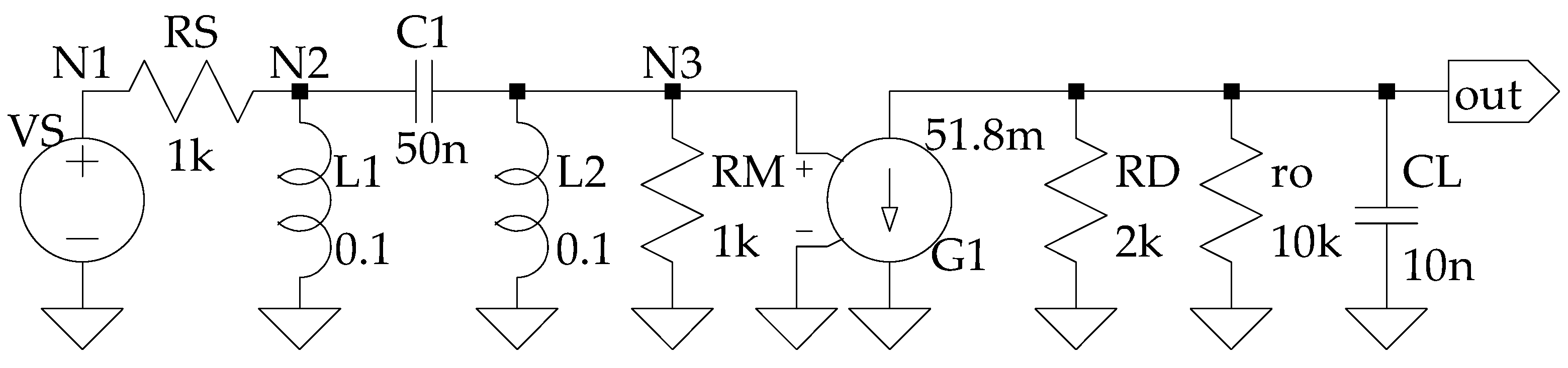
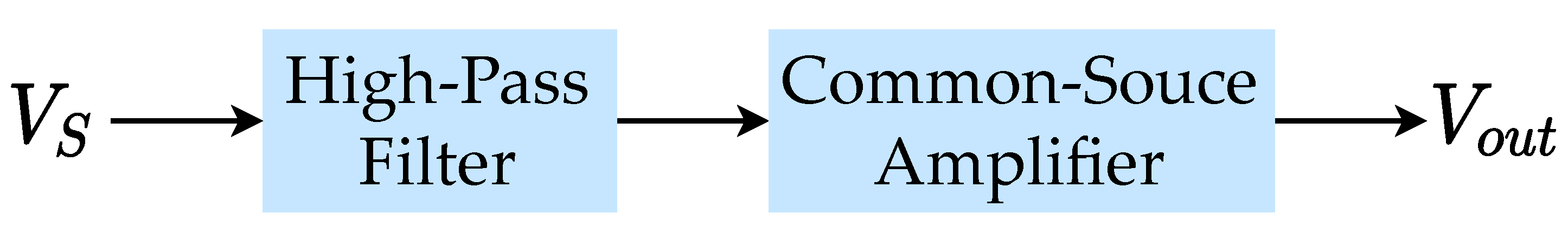
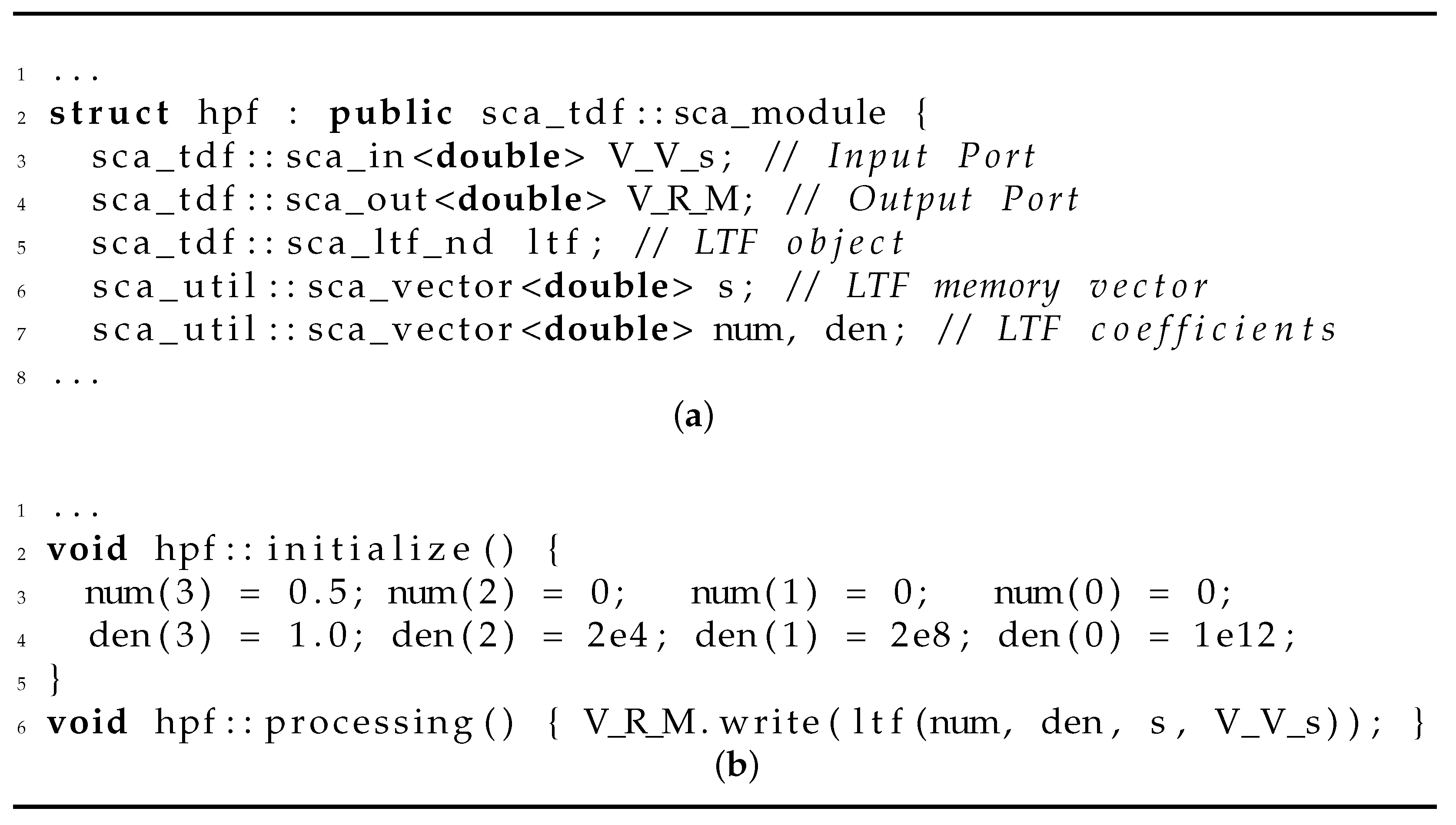
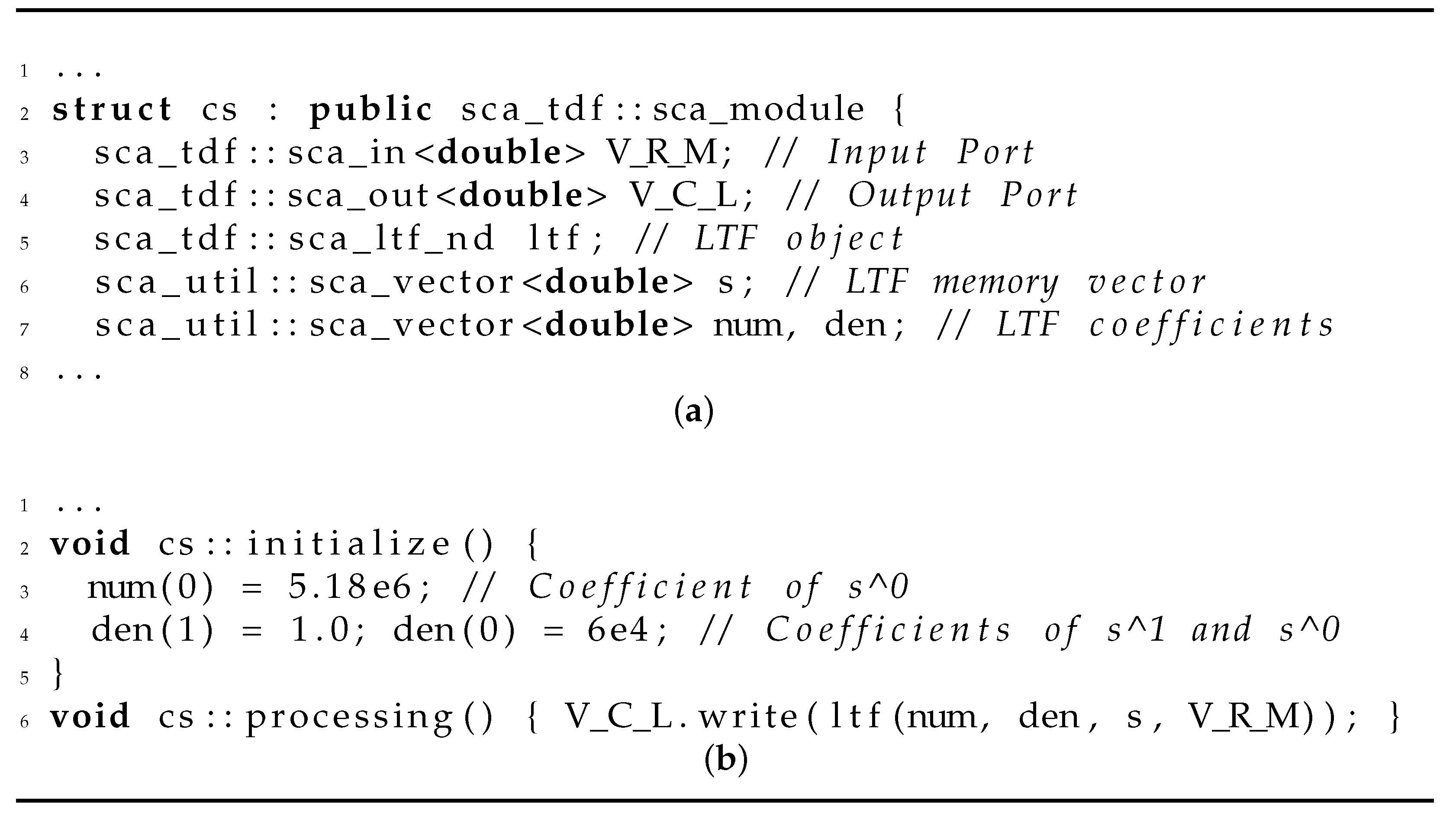
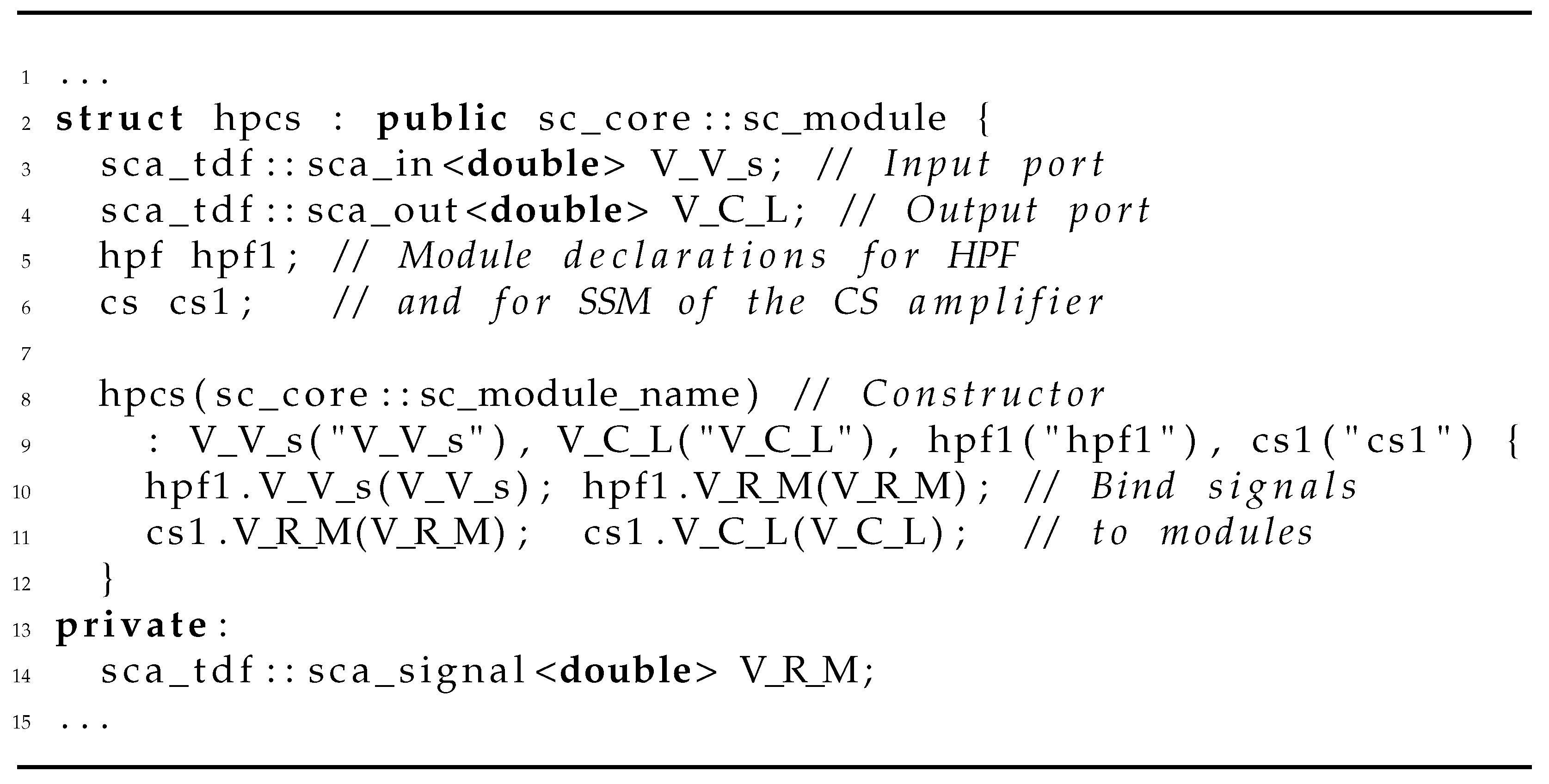
3.4. Motivating Example: Series-Connected HPF and SSM of Common-Source (CS) Amplifier

As our motivating example for equivalence checking, we consider a single-input (voltage of VS) single-output (voltage of out) system, consisting of a series-connected analog third-order passive HPF and an SSM of a CS amplifier with a capacitive load (Figure 5). The resistors RS, RM, and RD in the figure stand for source resistance, matching resistance, and drain resistance, respectively. The resistance ro models the channel-length modulation behavior of the MOSFET, whereas CL represents the load capacitance. The numbers of the nodes, N1, N2, and N3, are arbitrary. HPFs and amplifiers are typically used in audio crossovers. The HPF is designed to allow signals with a frequency higher than a certain cutoff frequency, and attenuate the signals with a frequency lower than that cutoff frequency.

The applicability of the methodology is indifferent to the specific values of the components, but for demonstration purposes, specific values were chosen for these circuits. The components of the HPF circuit are chosen such that it is of type Butterworth, which has a maximally flat response on the passband. The values of the design specifications are $10\times {10}^3$ rad/s ($1.592$ kHz) for the cutoff frequency and $0.5$ for the gain at the passband. The SSM represents the linear region of behavior of a CS amplifier with a gain of $-86.35$. A capacitive load of 10 nF is assumed at the output. The circuit is implemented in LTSpice [23] and exported as a netlist.

The behavioral block diagram of the circuit is given in Figure 6. The two blocks are represented by the LTFs of the HPF and of the CS amplifier’s SSM, which are given in Equation (4) and Equation (5), respectively.

$$\begin{array}{cc}\hfill H_{\mathrm{HPF}}\left(s\right)& =\frac{0.5s^3}{s^3+2\times {10}^4{s}^2+2\times {10}^{8}s+{10}^{12}}\hfill \end{array}$$

(4)

$$\begin{array}{cc}\hfill H_{\mathrm{CS}}\left(s\right)& =\frac{-5.18\times {10}^6}{s+6\times {10}^4}\hfill \end{array}$$

(5)

The coefficients of the HPF’s transfer function were calculated by transforming the prototype third-order low-pass Butterworth filter

$$H_{\mathrm{LPF}}\left(s\right)=\frac{1}{s^3+2s^2+2s+1}$$

(6)

to the high-pass form at the relevant cutoff frequency and by adjusting its passband gain. The transformation is achieved by replacing s in Equation (6) with $\frac{10\times {10}^3}{s}$, and the gain is simply adjusted by multiplying the LTF by 0.5. The coefficients of the CS amplifier’s LTF are determined from its SSM using modified nodal analysis [24].

The system-level model of the circuit is based on this block diagram and is implemented in SystemC AMS. Two TDF MoC modules are used to model the two blocks. The implementation of the HPF and the CS amplifier is given in Figure 7 and Figure 8, respectively. As both blocks are represented by single LTFs, they are implemented by a single LTF object sca_tdf::sca_ltf_nd. The modules are then connected in the parent module hpcs given in Figure 9. The declarations of the modules are at lines 5 and 6, and they are connected with the signal V_R_M at lines 10 and 11.

To increase our confidence in the system-level and SPICE-level implementations shown above, we introduce our graph-based equivalence checking procedure in the next section.

4. Signal-Flow Driven Equivalence Checking Methodology

In this section, we propose an SFG-based equivalence checking methodology for system-level and SPICE-level SISO linear analog circuit models. First, we describe the overview of our proposed methodology, followed by techniques to create and optimize an SFG. In the end, we illustrate our methodology using our motivating example from Section 3.4.

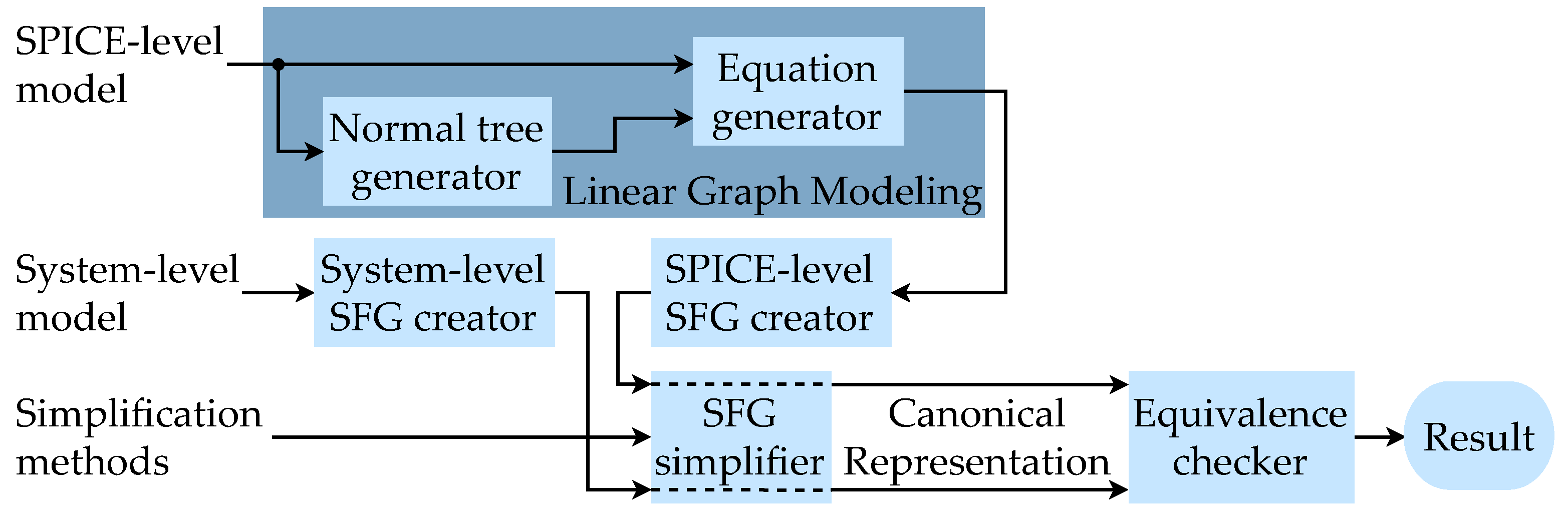
4.1. Methodology Overview

A block-diagram overview of our methodology for equivalence checking between system-level and SPICE-level models is seen in Figure 10. To generate a complete set of equations from the netlist, we use the linear graph modeling method [25], which consists of a normal tree generator and an equation generator. We chose this method of analysis as it preserves the structure of the circuit the best and loses the least amount of information. We then create an SFG of the circuit with our SPICE-level SFG creator and an SFG of the SystemC AMS description with our system-level SFG creator. We then reduce these SFGs to a minimal canonical form with our SFG simplifier. The simplification methods of the SFG simplifier are detailed in Section 4.4 and consist of the removal of a non-input node, parallel edge elimination, and reflexive edge elimination. Our equivalence checker compares the two canonical SFGs. All these manipulations and transformations are statically performed and are not simulation-based.

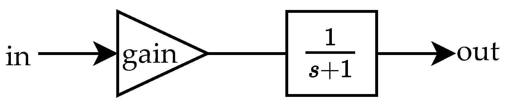
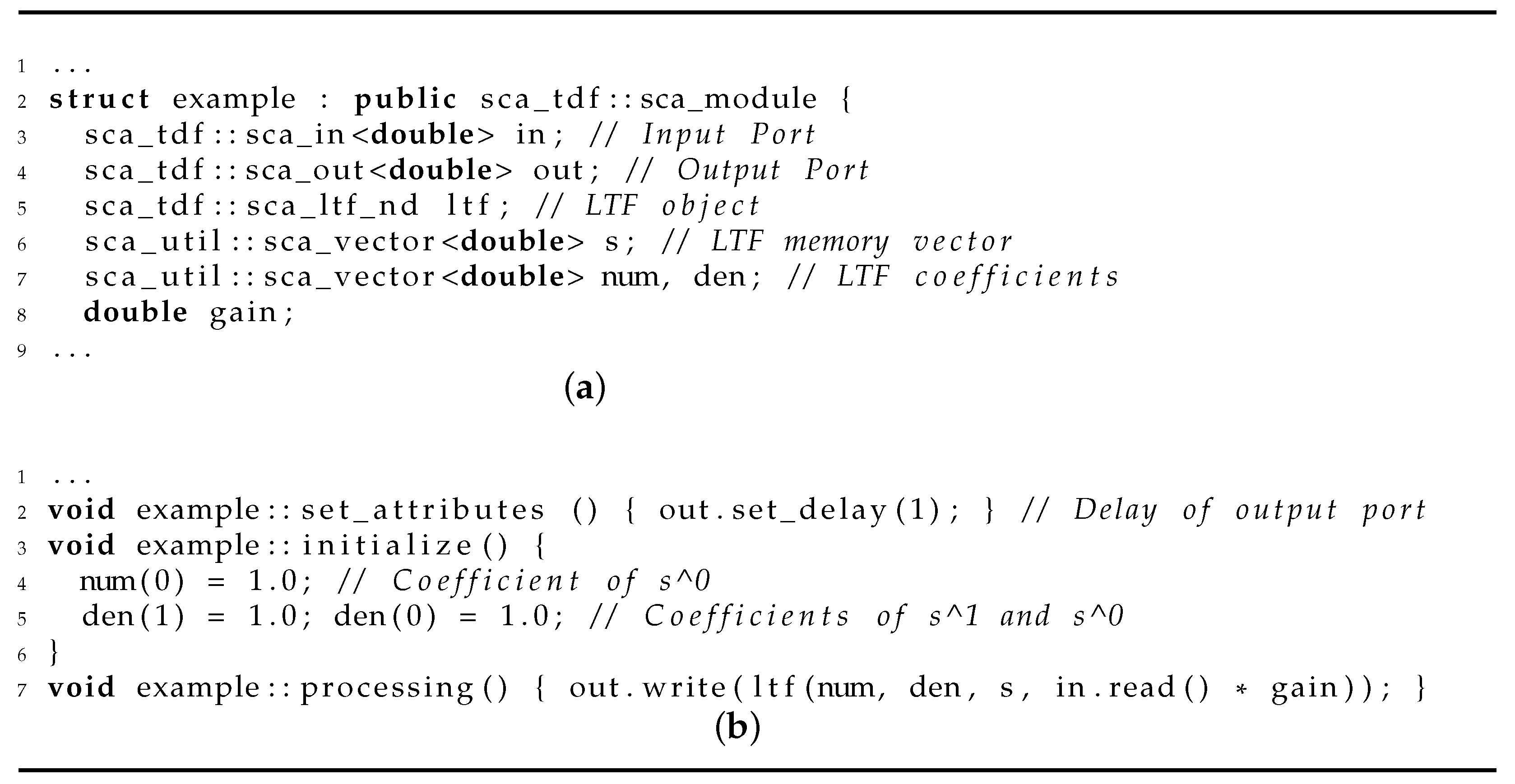
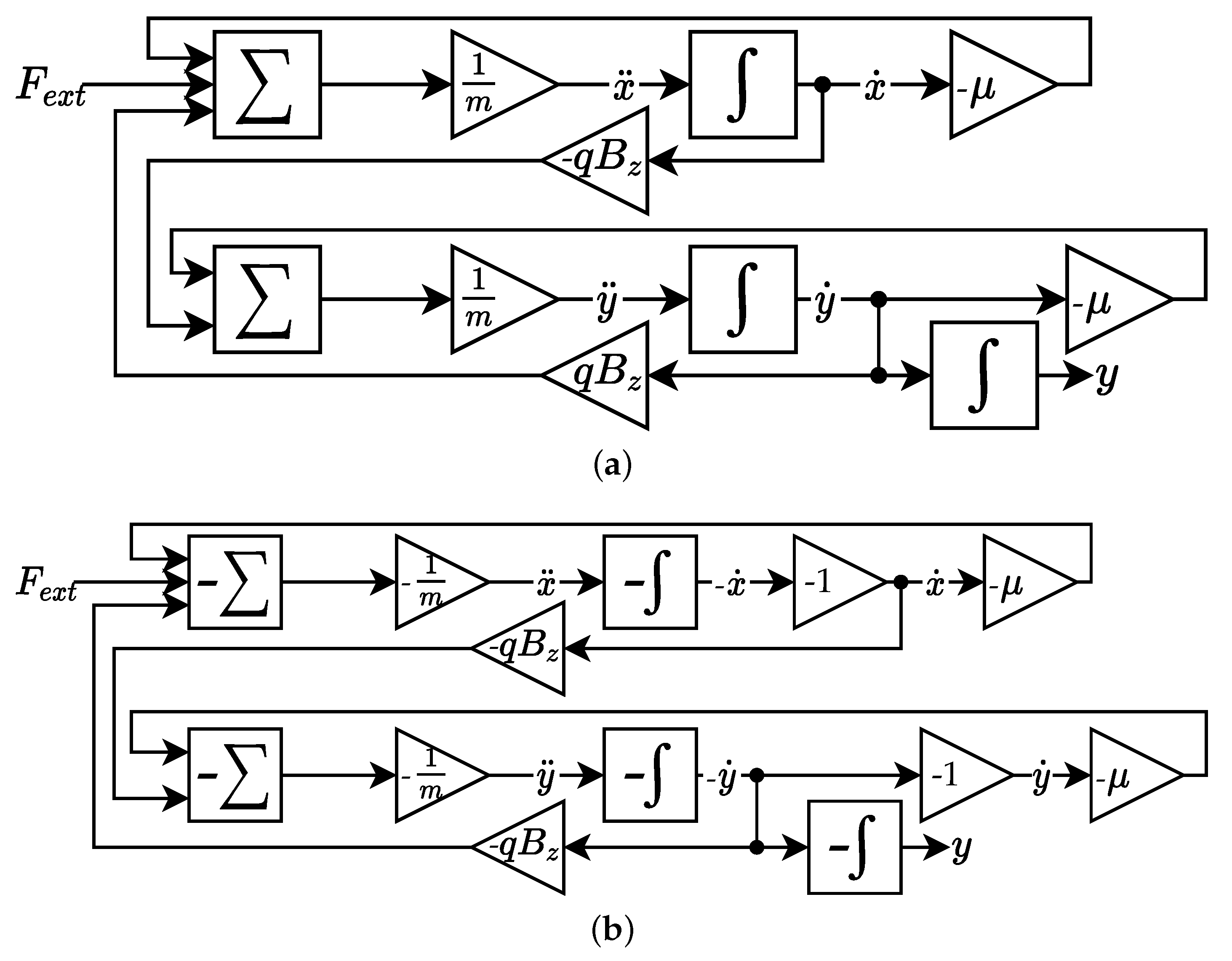
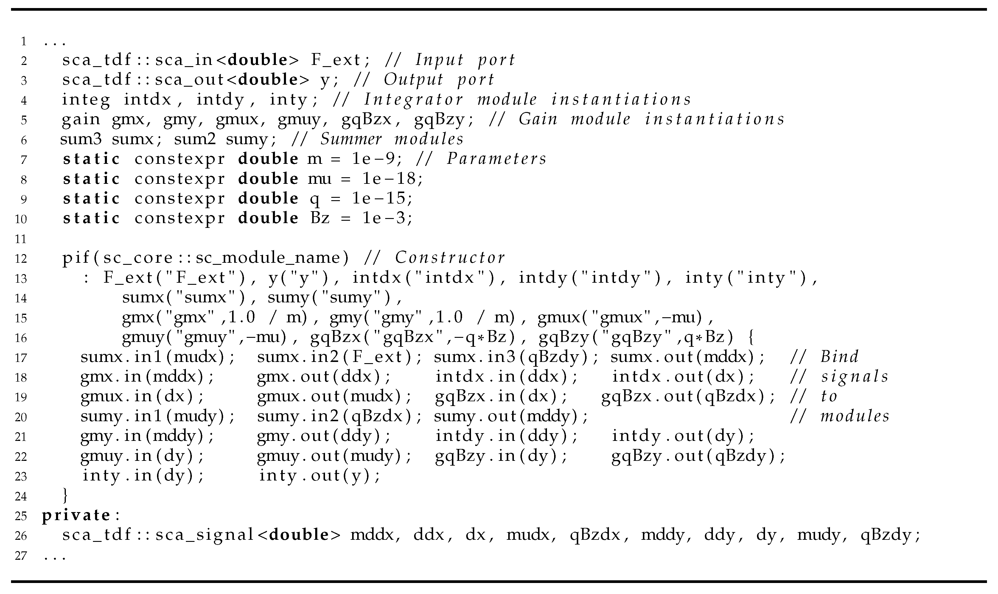
4.2. Creating the Signal-Flow Graph from System-Level Descriptions

The proposed methodology supports complex system-level behavioral descriptions as long as these use linear operations only. Linear operations include addition, multiplication by a constant, and LTF operators, which are enough to represent any linear SISO system. As programming code is already written in explicit form, SystemC AMS descriptions for system-level implementations are already in the form of Equation (2). Only the LTF objects have a slightly different form. As explained in Section 3.3, the line given as “y = ltf(num, den, s, x)” is used to process the LTF object defined as “sca_tdf::sca_ltf_nd ltf” and represents the equation

$$y=\frac{num\left(s\right)}{den\left(s\right)}x$$

which is also in the form of Equation (2).

Equations in this form can be directly transformed into an SFG as explained in Section 3.1.

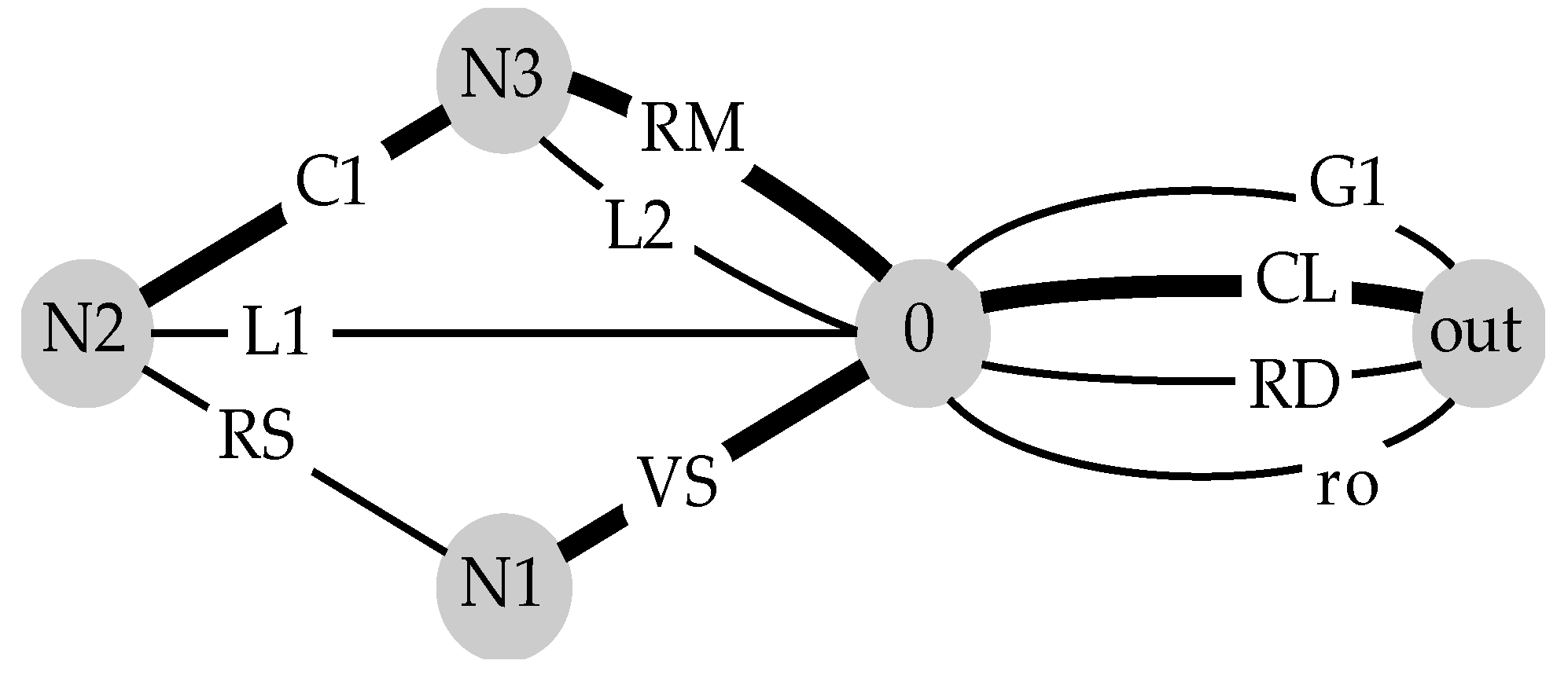
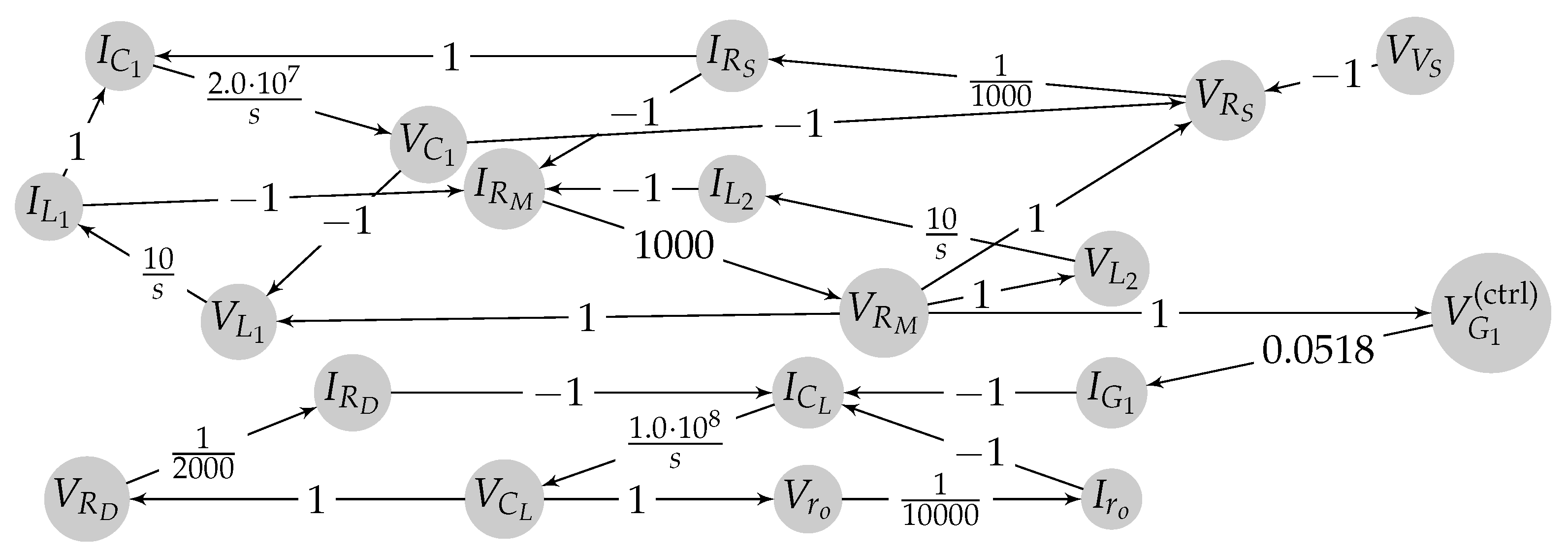
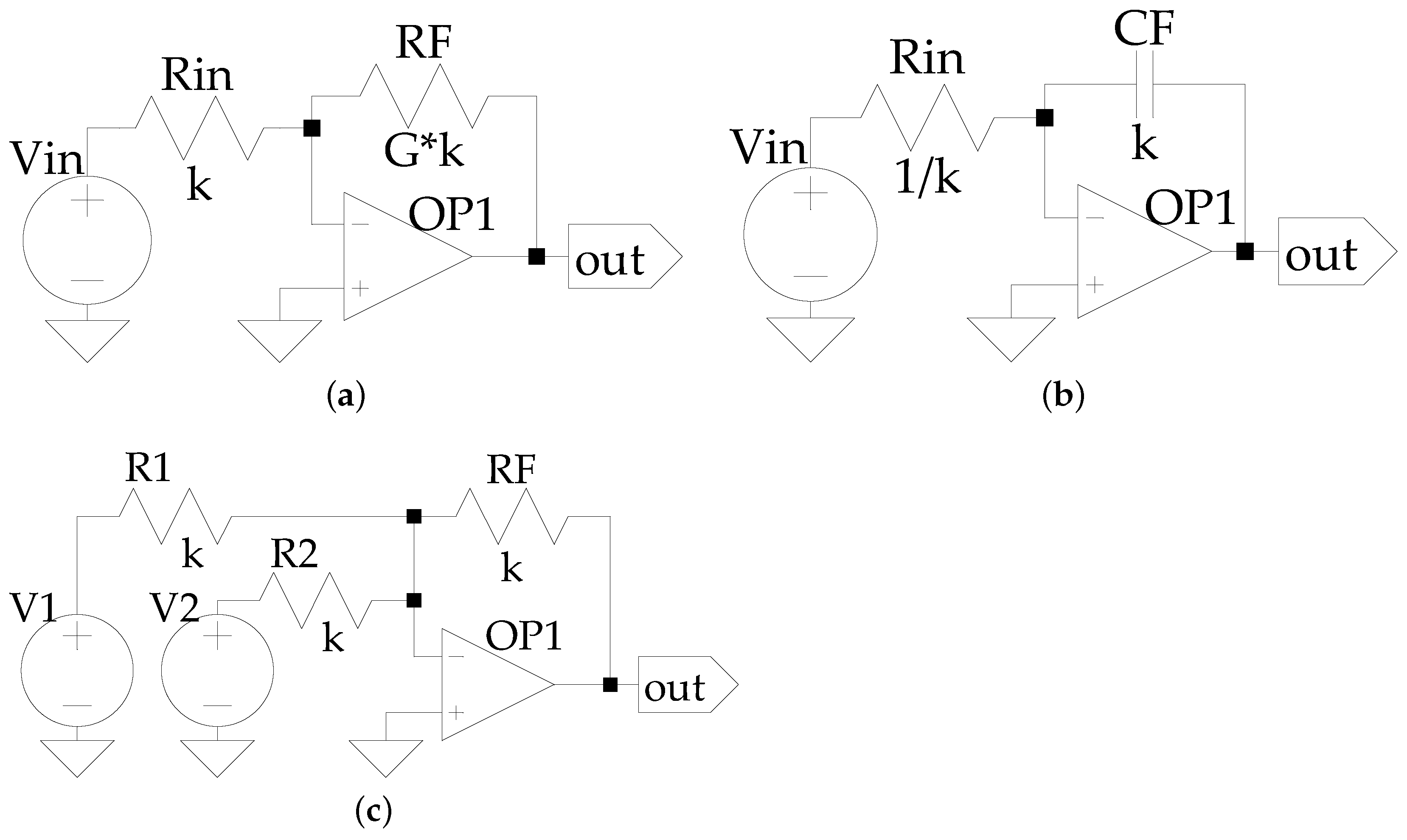
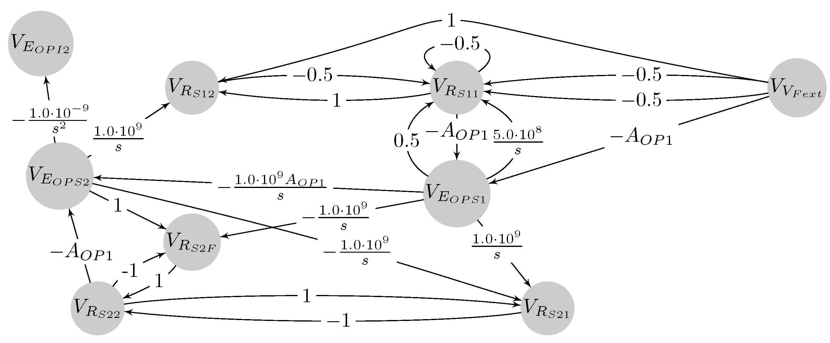
4.3. Creating the Signal-Flow Graph from SPICE-Level Descriptions

For the creation of the SPICE-level SFG, a set of linear explicit algebraic equations in the form of Equation (2) must be obtained from the SPICE-level model. There are various circuit analysis methods that can be used for this purpose, which use different methods and different sets of representative variables. In principle, various possible SFGs exist for a single circuit, as SFGs are created from sets of equations that were generated by one of these circuit analysis methods.

The linear graph modeling method that we use in our methodology uses the voltages on and currents through the circuit components as representative variables of the circuit. This is in contrast to nodal-analysis and loop-analysis, where the circuit equations are in terms of node voltages and loop currents, respectively.

The linear graph model determines how the circuit variables relate to each other by informing whether to focus on the explicit equations of a variable through elemental, compatibility (Kirchhoff’s voltage law), or continuity (Kirchhoff’s current law) equations. The first step of the linear graph modeling method is to create a normal tree, which is a special type of minimum spanning tree of the circuit graph. This is achieved by the normal tree generator by repetitively adding the edges of the circuit graph in the following order: Voltage sources, capacitors, resistors, inductors, and current sources.

Edges of the circuit graph that are not included in the normal tree are called the tree links of the normal tree. The normal tree must include voltage sources and may not include current sources. Inductors in the normal tree and capacitors in the tree links are dependent energy storage elements. Dependent energy storage elements are supported by the methodology and might be unavoidable due to the modeling approach, but could also point to a problem with the model.

For all unknown variables, an explicit expression is generated by the equation generator according to the following rules:

• Voltages of components on the normal tree, from elemental equations.
• Currents of components on the normal tree, from continuity equations.
• Voltages of components on the tree links, from compatibility equations.
• Currents of components on the tree links, from elemental equations.

When generating an explicit expression for the current of a component on the normal tree, the other currents in the continuity equation need to be from components on the tree links. These components can be found by temporarily removing the component on the normal tree from the normal tree, thereby splitting the normal tree into two connected components. Then, the continuity equation is generated with the currents of the components in the tree links that go from one connected component to the other.

Similarly, when generating an explicit expression for the voltage of a component on the tree links, the other voltages in the compatibility equation need to be from components on the normal tree. These components can be found by temporarily adding the component on the tree link to the normal tree and searching for a cycle. This cycle is then used for the compatibility equation.

This method generates equations in the form of Equation (2), which are used to construct an SFG as explained in Section 3.1.

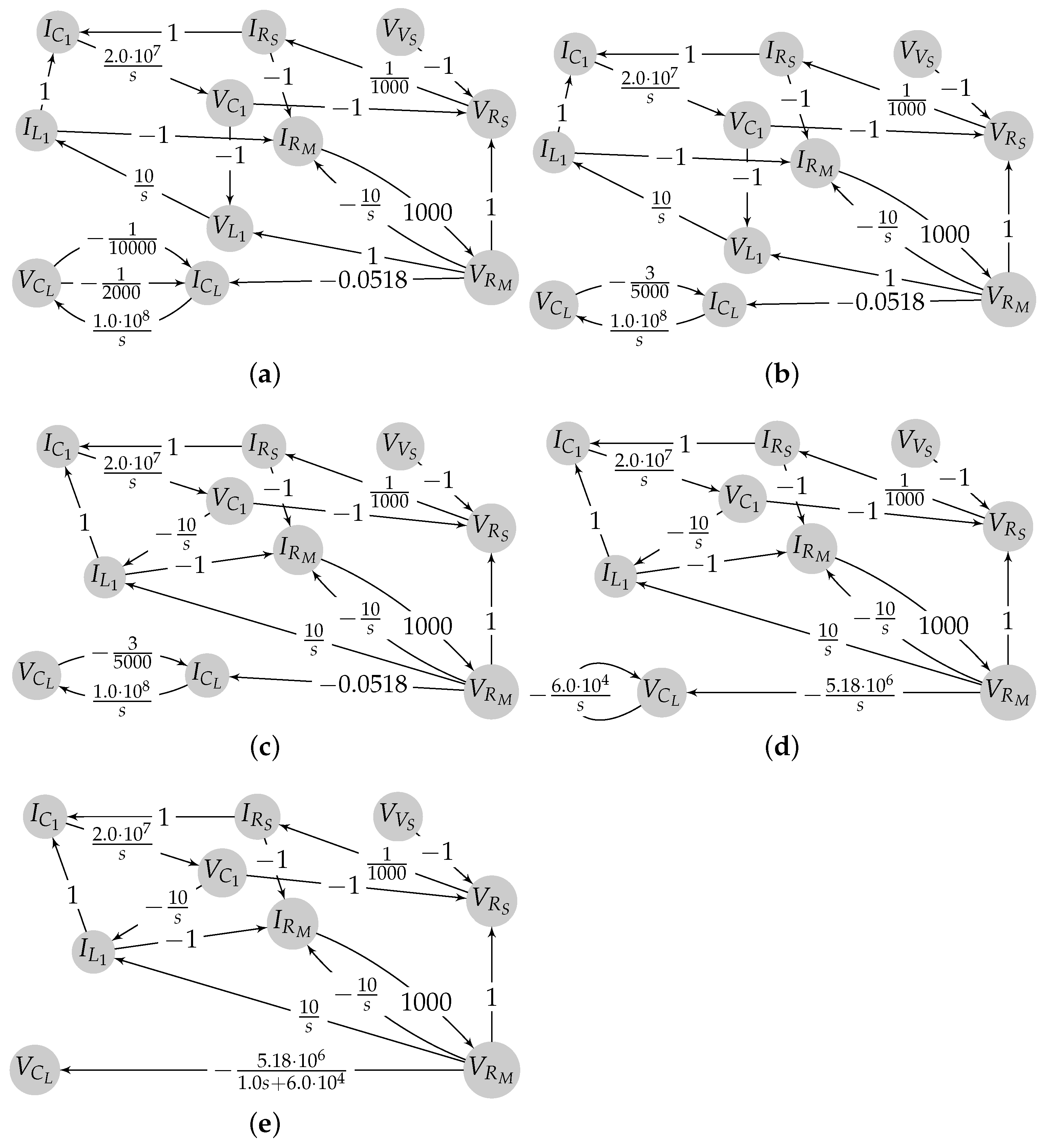
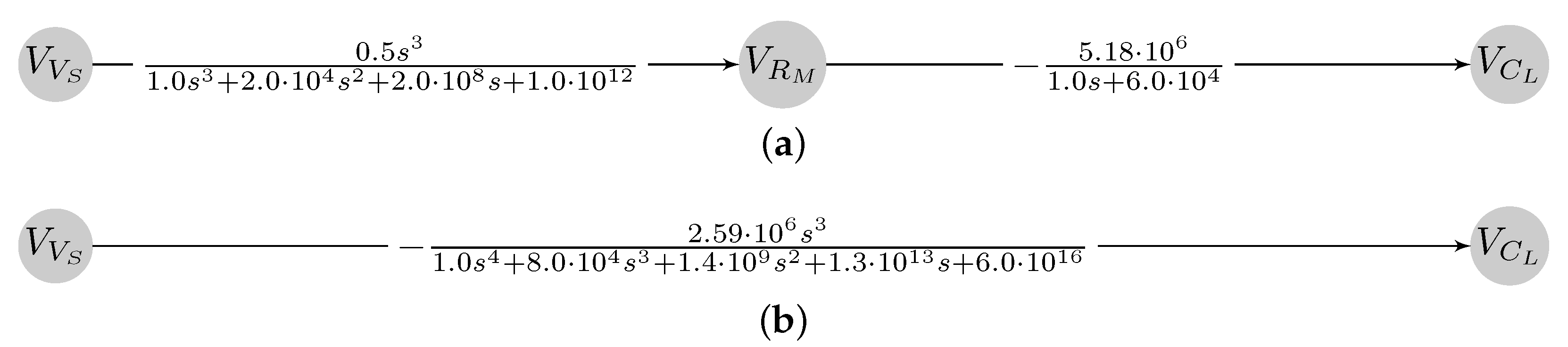
4.4. Reducing the Signal-Flow Graph

The created SFGs from the system-level and SPICE-level implementations are reduced to their canonical form by the block called “SFG simplifier”. The flowchart of the SFG simplification process is given in Figure 11 and consists of the simplification rules given in Section 3.2. These are applied by the SFG simplifier repeatedly in the given order until a minimal graph with only a single edge between its input and output nodes is obtained.

As SISO systems only have one input and one output node, and the process removes one node at every loop, the process is guaranteed to reduce the SFG to two nodes and terminate. Similarly, we can guarantee that only one edge will be left in the final SFG. After the final node removal, the only edges left in the SFG will be ones that go from the input node to the output node and reflexive edges at the output node. The edges from the input node to the output node are reduced to a single edge by unification. The reflexive edges are eliminated at the next step, which does not create any new edges. Therefore the returned SFG will have only a single edge.

4.5. Illustration

In this section, we illustrate our methodology on the series-connected circuit from Figure 5. As the first step of linear graph modeling, we obtain the circuit’s normal tree, shown with bold edges in Figure 12. Comparing this with the circuit in Figure 5, it is seen that it is indeed a minimum spanning tree by observing that all nodes of the circuit are present in the tree without forming any loops. It can also be seen that the priority order as explained in Section 4.3 was followed, as all voltages and capacitors of the circuit are present on the tree. The inclusion of RM in the normal tree instead of RS is arbitrary.

In the second step, we use this normal tree and the rules given in Section 4.3 to find the explicit Equations (7) and (8), which are required for building the SFG. In Equation (7), the equations for the components on the normal tree are given.

$$\begin{array}{cccc}\hfill V_{C1}& =\frac{1}{50\times {10}^{-9}s}{I}_{C1},\hfill & \hfill I_{C1}& =I_{RS}+I_{L1},\hfill \\ \hfill V_{RM}& ={10}^3{I}_{RM},\hfill & \hfill I_{RM}& =-I_{L1}-I_{L2}-I_{RS},\hfill \\ \hfill V_{CL}& =\frac{1}{10\times {10}^{-9}s}{I}_{CL},\hfill & \hfill I_{CL}& =-I_{G1}-I_{RD}-I_{ro},\hfill \\ \hfill & \hfill & \hfill I_{VS}& =-I_{RS}.\hfill \end{array}$$

(7)

whereas the equations for the components on the tree links are given in Equation (8).

$$\begin{array}{cccc}\hfill V_{RS}& =-V_{VS}-V_{C1}+V_{RM},\hfill & \hfill I_{RS}& =\frac{1}{{10}^3}{V}_{RS},\hfill \\ \hfill V_{L1}& =-V_{C1}+V_{RM},\hfill & \hfill I_{L1}& =\frac{1}{0.1s}{V}_{L1},\hfill \\ \hfill V_{L2}& =V_{RM},\hfill & \hfill I_{L2}& =\frac{1}{0.1s}{V}_{L2},\hfill \\ \hfill V_{RD}& =V_{CL},\hfill & \hfill I_{RD}& =\frac{1}{2\times {10}^3}{V}_{RD},\hfill \\ \hfill V_{ro}& =V_{CL},\hfill & \hfill I_{ro}& =\frac{1}{10\times {10}^3}{V}_{ro},\hfill \\ \hfill V_{G1}& =V_{CL}.\hfill \end{array}$$

(8)

While the linear graph modeling approach uses substitution from this point on, we leave the equations as they are, and construct an SFG right away to preserve the structure of the circuit. Equations (7) and (8) are in the form of Equation (2), from which the SFG given in Figure 13 can be created.

This SFG is then transformed according to the rules given in Section 4.4. An example of parallel edge unification is seen in the ninth step of the simplification process, where the parallel edges from $V_{C_L}$ to $I_{C_L}$ in Figure 14a are merged to find the single edge in Figure 14b. The next two steps are examples of non-input node removal, where the nodes $V_{L_1}$ and $I_{C_L}$ were removed to obtain the graphs in Figure 14c and Figure 14d, respectively. The simplification step from Figure 14d to Figure 14e is an example of reflexive edge elimination, where the reflexive edge at $I_{C_L}$ was removed. After the successive removal of 17 nodes according to these rules, the minimal SFG in Figure 15 is obtained. The numbers in these figures were printed with reduced floating-point precision due to space considerations.

Finding the system-level SFG given in Figure 16a from the system-level description given in Figure 7, Figure 8 and Figure 9 is trivial, as the system-level models were already described as LTFs. The simplification of this SFG only involves the removal of the node $V_{R_M}$, after which the canonical form in Figure 16b is obtained. For equivalence checking, it is observed that the SFG in Figure 16b is equal to the SFG in Figure 15.

The successful application of our methodology to our motivating example shows that it works. In the next section, we apply our methodology to a more complex example to illustrate its general applicability.

5. Experimental Evaluation

In this section, we demonstrate the general applicability of our proposed system-level and SPICE-level equivalence checking methodology by applying it to an example circuit from a different domain, namely analog computing. First, the experimental setup is briefly discussed. Later, we demonstrate our methodology described in Section 4 by creating and simplifying SFGs for the system-level and SPICE-level implementations of the circuit. We then compare the simplified canonical SFGs to check equivalence.

5.1. Experimental Setup

For this demonstration, we use an analog computing circuit, slightly changed from its original in [26], which simulates the behavior of a charged particle under a magnetic field. The slight change was the addition of an external force ($F_{ext}$), which was included as the original circuit had no input. The charged particle in this system is constrained to a two-dimensional plane, and the magnetic field is perpendicular to this plane. The force $F_{ext}$ that is acting on the particle has a fixed direction and is applied parallel to the plane. If we consider a Cartesian coordinate system on the plane, with its x-axis parallel to $F_{ext}$, we denote the position of the particle on the x-axis as x and on the y-axis as y. As our methodology is constrained to SISO systems, we only use y as our output.

The equations describing the dynamics of the system are

$$\begin{array}{cc}\hfill m\ddot{x}& =q\dot{y}{B}_z-\mu \dot{x}+F_{ext}\hfill \\ \hfill m\ddot{y}& =-q\dot{x}{B}_z-\mu \dot{y}\hfill \end{array}$$

(9)

from which the system-level block diagram of the circuit seen in Figure 17a is generated. The numerical values for the parameters are chosen as 10${}^{-9}$ g for m, 10${}^{-18}$ g s${}^{-1}$ for $\mu$, 10${}^{-15}$ C for q, and 10${}^{-3}$ T for $B_z$.

The system is implemented in SystemC AMS in a hierarchical manner. The top-level module which instantiates and connects all the sub-modules is given in Figure 18. All summer, gain, and integrator blocks are implemented as TDF MoC modules. The integral operations in the block diagram can be represented by LTFs with the value $\frac{1}{s}$. These are implemented with sca_tdf::sca_ltf_nd objects in a similar fashion to the previous examples. The gains and summers are implemented with multiplication and addition operators. The gain values of the gain blocks are specified in the constructor of the top-level module at lines 15 and 16.

The SPICE-level model of the circuit is implemented by using template circuits that act as inverting summers, inverting integrators, and inverting gains. The template circuits are given in Figure 19. The op-amps are assumed ideal and non-saturating. The parameter k in the template circuits can be chosen freely and does not affect the circuit behavior as the output resistances of the op-amps are assumed zero. The inverting summer circuit implements the system-level behavior of $-\sum$ and can be extended with more inputs. The gain of the inverting gain circuit is $-G$ and can be adjusted by changing the parameter G. The system-level blocks of $-\frac{1}{m}$, $-q{B}_z$, $-\mu$, and $-1$ can be realized with this inverting gain circuit by setting G to $\frac{1}{m}$, $q{B}_z$, $\mu$, and 1, respectively. Finally, the inverting integrator circuit implements the system-level behavior of $-\int$. As these template circuits are inverting the input, the system-level model was readjusted to the model given in Figure 17b. The SPICE-level implementation could then be realized by plugging the template circuits into respective blocks in the block diagram. This is allowed, as the output resistances of all the template circuits in Figure 19 are equal to the output resistances of the op-amps, and therefore zero. The final SPICE-level implementation consists of 26 resistors, 3 capacitors, and 13 op-amps.

5.2. Equivalence Checking

The process used to create the SFG from the SPICE-level circuit once again consists of obtaining the normal tree, finding the explicit equations for the variables of the circuit, and putting these equations together to create the SFG. The obtained SFG initially had 85 nodes and 132 edges.

The graph reduction rules given in Section 4.4 are then applied to this SFG for simplification. An intermediate graph with nine nodes, which has two sets of parallel edges and one reflexive edge, is seen in Figure 20. The symbol $A_{OP1}$ stands for the op-amp gain, which is assumed infinite. The final canonical SFG from the simplification process is given in Figure 21.

The SystemC AMS code of the system-level implementation can be transformed into the system-level SFG in Figure 22a as explained in Section 3.1. The names of the nodes are the names of the signals in the SystemC AMS code. Although the names of the signals do not matter for the methodology to work, they were chosen to aid comprehension. The character m stands for the mass m, d stands for derivative, mu stands for $\mu$, and Bz stands for $B_z$. After the simplification process and after substituting numeric values, the canonical form in Figure 22b is obtained. For equivalence checking, the LTFs at the only edges of the SFGs in Figure 22b and Figure 21 are compared. It is seen that these are equivalent, which implies the behavioral equivalency between the system-level model and the SPICE-level model. Therefore, any result generated with the system-level model can be analyzed more confidently.

The total application time it took to apply the methodology to the analog simulator for a particle in a magnetic field was 4.9 s, whereas when applied to the series-connected HPF and CS amplifier circuit it was 1.3 s. The computations were conducted on an octa-core AMD Ryzen 7 PRO 4750U with 32 GB RAM.

By successfully applying our methodology to an analog computer with complex system-level and SPICE-level implementations, we have demonstrated the general applicability and scalability of our approach. Next, we will summarize the main conclusions and discuss possible research directions for the future.

6. Conclusions

In this work, we combined various analysis and modification techniques in a novel way to create a graph-based, formal equivalence checking method. We extended our novel equivalence methodology to behavioral system-level models that go beyond single LTFs. We have also extended the applicability of our methodology to the general class of SISO linear analog circuits. To achieve this, we create system-level SFGs from SystemC AMS descriptions and use linear graph modeling on SPICE-level models to create SPICE-level SFGs. To compare these graphs, we use graph reduction techniques to transform them into a common canonical form. By observing the successful application of the methodology to the provided examples, we learned that using graphs to show formal equivalency is a viable option that merits further investigation.

The methods presented in this article can be extended in multiple ways. As a slight difference between the SPICE-level and system-level models might be tolerable, the method can be modified to generate an error value between the models. For this, the poles and zeros of the transfer function in the canonical SFGs can be compared. Additionally, the current application scope of this work is restricted to linear analog circuits. A generalization to nonlinear circuits should be investigated. Another interesting research direction is to leverage the graph-based representation using established search methods to map possible bugs between the two models. Furthermore, the method can be extended to multiple-input multiple-output systems and can be used to analyze systems with external noise input.

References

1. Barnasconi, M. SystemC AMS Extensions: Solving the Need for Speed; DAC Knowledge Center: San Francisco, CA, USA, 2010. [Google Scholar]
2. Nagel, L.W. SPICE-Simulation Program with Integrated Circuit Emphasis; Electronics Research Laboratory, University of California: Berkeley, CA, USA, 1973. [Google Scholar]
3. Grimm, C.; Barnasconi, M.; Vachoux, A.; Einwich, K. An Introduction to Modeling Embedded Analog/Mixed-Signal Systems Using SystemC AMS Extensions; Open SystemC Initiative: Sunnyvale, CA, USA, 2008. [Google Scholar]
4. Barnasconi, M.; Grimm, C.; Damm, M.; Einwich, K.; Louërat, M.; Maehne, T.; Pecheux, F.; Vachoux, A. SystemC AMS Extensions User’s Guide; Accellera Systems Initiative: Elk Grove, CA, USA, 2010. [Google Scholar]
5. Barnasconi, M.; Einwich, K.; Grimm, C.; Maehne, T.; Vachoux, A. Advancing the SystemC Analog/Mixed-Signal (AMS) Extensions; Open SystemC Initiative: Sunnyvale, CA, USA, 2011. [Google Scholar]
6. Pêcheux, F.; Grimm, C.; Maehne, T.; Barnasconi, M.; Einwich, K. SystemC AMS Based Frameworks for Virtual Prototyping of Heterogeneous Systems. In Proceedings of the 2018 IEEE International Symposium on Circuits and Systems (ISCAS), Florence, Italy, 27–30 May 2018; pp. 1–4. [Google Scholar]
7. Drechsler, R. (Ed.) Advanced Formal Verification; Kluwer Academic Publishers: Alphen aan den Rijn, The Netherlands, 2004. [Google Scholar]
8. Molitor, P.; Mohnke, J. Equivalence Checking of Digital Circuits: Fundamentals, Principles, Methods; Springer Science & Business Media: Berlin/Heidelberg, Germany, 2007. [Google Scholar]
9. Drechsler, R. Formal System Verification; Springer: Berlin/Heidelberg, Germany, 2018. [Google Scholar]
10. Zaki, M.H.; Tahar, S.; Bois, G. Formal Verification of Analog and Mixed Signal Designs: A Survey. Microelectron. J. 2008, 39, 1395–1404. [Google Scholar] [CrossRef] [Green Version]
11. Tarraf, A.; Hedrich, L.; Kochdumper, N.; Rechmal-Lesse, M.; Olbrich, M. Equivalence Checking Methods for Analog Circuits Using Continuous Reachable Sets. In Proceedings of the 2020 IEEE Computer Society Annual Symposium on VLSI (ISVLSI), Limassol, Cyprus, 6–8 July 2020; pp. 7–12. [Google Scholar] [CrossRef]
12. Hedrich, L.; Barke, E. A Formal Approach to Nonlinear Analog Circuit Verification. In Proceedings of the IEEE International Conference on Computer Aided Design (ICCAD), San Jose, CA, USA, 5–9 November 1995; pp. 123–127. [Google Scholar] [CrossRef]
13. Hedrich, L.; Hartong, W. Approaches to Formal Verification of Analog Circuits. In Low-Power Design Techniques and CAD Tools for Analog and RF Integrated Circuits; Wambacq, P., Gielen, G., Gerrits, J., van Leuken, R., de Graaf, A., Nouta, R., Eds.; Springer: Boston, MA, USA, 2001; pp. 155–191. [Google Scholar] [CrossRef]
14. Hartong, W.; Klausen, R.; Hedrich, L. Formal Verification for Nonlinear Analog Systems: Approaches to Model and Equivalence Checking. In Advanced Formal Verification; Drechsler, R., Ed.; Springer: Boston, MA, USA, 2004; pp. 205–245. [Google Scholar] [CrossRef]
15. Steinhorst, S.; Hedrich, L. Advanced Methods for Equivalence Checking of Analog Circuits with Strong Nonlinearities. Form. Methods Syst. Des. 2010, 36, 131–147. [Google Scholar] [CrossRef]
16. Singh, A.; Li, P. On Behavioral Model Equivalence Checking for Large Analog/Mixed Signal Systems. In Proceedings of the 2010 IEEE/ACM International Conference on Computer-Aided Design (ICCAD), San Jose, CA, USA, 7–11 November 2010; pp. 55–61. [Google Scholar] [CrossRef] [Green Version]
17. Ain, A.; Sanyal, S.; Dasgupta, P. A Framework for Automated Feature Based Mixed-Signal Equivalence Checking. In Proceedings of the VLSI Design and Test; Communications in Computer and Information Science; Kaushik, B.K., Dasgupta, S., Singh, V., Eds.; Springer: Singapore, 2017; pp. 779–791. [Google Scholar] [CrossRef]
18. Saglamdemir, M.O.; Dundar, G.; Sen, A. An Analog Behavioral Equivalence Checking Methodology for Simulink Models and Circuit Level Designs. In Proceedings of the 2015 International Conference on Synthesis, Modeling, Analysis and Simulation Methods and Applications to Circuit Design (SMACD), Istanbul, Turkey, 7–9 September 2015; pp. 1–4. [Google Scholar] [CrossRef]
19. Coskun, K.C.; Hassan, M.; Drechsler, R. Equivalence Checking of System-Level and SPICE-Level Models of Linear Analog Filters. In Proceedings of the Design and Diagnostics of Electronic Circuits and Systems (DDECS), Prague, Czech Republic, 6–8 April 2022. [Google Scholar]
20. Mason, S.J. Feedback Theory-Some Properties of Signal Flow Graphs. Proc. IRE 1953, 41, 1144–1156. [Google Scholar] [CrossRef]
21. Robichaud, L.P.A. Signal Flow Graphs and Applications; Prentice Hall: Englewood Cliffs, NJ, USA, 1962. [Google Scholar]
22. Rasim, F.R.; Sattler, S.M. Analysis of Electronic Circuits with the Signal Flow Graph Method. Circuits Syst. 2017, 8, 261–274. [Google Scholar] [CrossRef] [Green Version]
23. Analog Devices. LTspice. Available online: https://www.analog.com/en/design-center/design-tools-and-calculators/ltspice-simulator.html (accessed on 23 March 2022).
24. Ho, C.W.; Ruehli, A.; Brennan, P. The modified nodal approach to network analysis. IEEE Trans. Circuits Syst. 1975, 22, 504–509. [Google Scholar]
25. Rowell, D.; Wormley, D.N. System Dynamics: An Introduction; Prentice Hall: Upper Saddle River, NJ, USA, 1997. [Google Scholar]
26. Ulmann, B. Analog and Hybrid Computer Programming; Walter de Gruyter GmbH & Co KG: Berlin, Germany, 2020. [Google Scholar]
Figure 1. The Signal-Flow Graph (SFG) corresponding to Equation (3).
Chips 01 00006 g001
Figure 2. The SFG corresponding to Equation (3) (a) after removal of node x 1 , (b) after parallel edge unification, and (c) after removal of the reflexive edge at node x 2 .
Chips 01 00006 g002
Figure 3. Introductory example: Series-connected gain and integrator.
Chips 01 00006 g003
Figure 4. System-level behavioral model of the example in Figure 3 implemented in SystemC AMS with (a) example.h and (b) example.cpp.
Chips 01 00006 g004
Figure 5. Motivating example: Series-connected High-Pass Filter (HPF) and small-signal model (SSM) of common-source (CS) amplifier with components Resistor (R), Capacitor (C), Inductor (L), and Voltage-Dependent Current Source (G1).
Chips 01 00006 g005
Figure 6. System-level block diagram of the series connection of an HPF and the SSM model of a CS amplifier.
Chips 01 00006 g006
Figure 7. System-level behavioral model of the HPF implemented in SystemC AMS with (a) hpf.h and (b) hpf.cpp.
Chips 01 00006 g007
Figure 8. System-level behavioral model of the CS amplifier’s SSM implemented in SystemC AMS with (a) cs.h and (b) cs.cpp.
Chips 01 00006 g008
Figure 9. System-level series connection of the HPF and the CS amplifier’s SSM implemented in SystemC AMS.
Chips 01 00006 g009
Figure 10. Overview of the proposed equivalence checking methodology.
Chips 01 00006 g010
Figure 11. Overview of SFG simplification process.
Chips 01 00006 g011
Figure 12. Graph of the series-connected HPF and CS amplifier circuit. The normal tree is emphasized with bold edges.
Chips 01 00006 g012
Figure 13. Initial SFG of the series-connected HPF and CS amplifier circuit.
Chips 01 00006 g013
Figure 14. Some results from the simplification process: (a) The SFG after eight simplification steps. (b) The SFG after parallel edges in the previous SFG are merged. (c) The SFG after removal of V L 1 . (d) The SFG after removal of I C L . (e) The SFG after the reflexive edge in the previous SFG is removed.
Chips 01 00006 g014
Figure 15. Reduced SFG of the series-connected HPF and CS amplifier circuit.
Chips 01 00006 g015
Figure 16. (a) Initial SFG and (b) reduced SFG of the system-level model of the HPF and CS amplifier circuit.
Chips 01 00006 g016
Figure 17. (a) System-level block diagram of the analog simulator for a particle in a magnetic field. (b) System-level block diagram, adjusted for SPICE-level implementation. The parameters of the simulator are: charge (q) and mass (m) of the particle, magnitude of the field ( B z ), and coefficient of the viscous friction ( μ ).
Chips 01 00006 g017
Figure 18. System-level behavioral model of the analog simulator for a particle in a magnetic field implemented in SystemC AMS.
Chips 01 00006 g018
Figure 19. Template circuits for (a) inverting gain, (b) inverting integrator, and (c) inverting summer.
Chips 01 00006 g019
Figure 20. An intermediate result from the simplification process of the analog simulator for a particle in a magnetic field.
Chips 01 00006 g020
Figure 21. Reduced SFG of the analog simulator for a particle in a magnetic field.
Chips 01 00006 g021
Figure 22. (a) Initial symbolic SFG and (b) reduced SFG with numerical substitutions of the system-level model of the analog simulator for a particle in a magnetic field.
Chips 01 00006 g022