Article

Parametric Stochastic Modeling of Particle Descriptor Vectors for Studying the Influence of Ultrafine Particle Wettability and Morphology on Flotation-Based Separation Behavior

1
Institute of Stochastics, University Ulm, 89069 Ulm, Germany
2
Helmholtz-Zentrum Dresden-Rossendorf, Helmholtz Institute Freiberg for Resource Technology, 09599 Freiberg, Germany
*
Author to whom correspondence should be addressed.
Powders 2023, 2(2), 353-371; https://doi.org/10.3390/powders2020021
Submission received: 24 February 2023 / Revised: 29 March 2023 / Accepted: 9 May 2023 / Published: 11 May 2023

Abstract

:
Practically all particle separation processes depend on more than one particulate property. In the case of the industrially important froth flotation separation, these properties concern wettability, composition, size and shape. Therefore, it is useful to analyze different particle descriptors when studying the influence of particle wettability and morphology on the separation behavior of particle systems. A common tool for classifying particle separation processes are Tromp functions. Recently, multivariate Tromp functions, computed by means of non-parametric kernel density estimation, have emerged which characterize the separation behavior with respect to multidimensional vectors of particle descriptors. In the present paper, an alternative parametric approach based on copulas is proposed in order to compute multivariate Tromp functions and, in this way, to characterize the separation behavior of particle systems. In particular, bivariate Tromp functions for the area-equivalent diameter and aspect ratio of glass particles with different morphologies and surface modification have been computed, based on image characterization by means of mineral liberation analysis (MLA). Comparing the obtained Tromp functions with one another reveals the combined influence of multiple factors, in this case particle wettability, morphology and size, on the separation behavior and introduces an innovative approach for evaluating multidimensional separation. In addition, we extend the parametric copula-based method for the computation of multivariate Tromp functions, in order to characterize separation processes, also in the case when image measurements are not available for all separated fractions.

1. Introduction

Considering the increasing amount of natural resources needed for everyday life, mining and recycling industries are permanently aiming for the optimization of existing processes and the development of novel technologies in order to improve the yield of valuable materials. One of the most important techniques in the mining industry for the processing of fine mineral particles (i.e., particles within the size range from 20   μ m to 200   μ m ) is flotation. This separation technique exploits the differences in wettability of various minerals, i.e., particles that are rather hydrophobic will attach to air bubbles and can be recovered as a froth, while rather hydrophilic particles remain in the suspension. However, in recent years it has been shown that other particle properties, e.g., given by descriptors of their size or shape, can also influence the separation process. Studies, which were focusing on the suspension zone during flotation, demonstrated that irregularly shaped particles have higher flotation recoveries when compared to rather spherical particles, since it is assumed that their sharp edges facilitate the rupture of the liquid film between the particle and the bubble [1,2,3,4]. This is supported by latest research including discrete element method simulations of particle-bubble interactions comparing spheres and irregularly shaped particles [5]. On the other hand, studies focusing on the froth zone did not yield such clear results, since some studies stated that the entrainment of unwanted gangue particles increases with particle roundness, whereas other studies claimed that the entrainment is higher for elongated particles [6,7,8]. Regarding particle size, it is known that flotation is most efficient for particles with intermediate size ranges. The flotation of very fine particles (smaller than 10   μ m ) is a challenging task and is accompanied by high levels of entrainment or slime coating, resulting in low grade concentrates [9,10,11,12].
In order to improve the separation efficiency for particle systems with a high amount of fines, a novel flotation apparatus has been designed, see Section 2.2 for details. It combines the advantages of agitator-type froth flotation, i.e., high turbulences for efficient particle-bubble collisions, and column flotation, i.e., reducing entrainment due to the fractionating effect of the column. Flotation experiments were carried out using simple particle systems consisting of magnetite as the non-floatable and glass particles with varying morphologies and with three different wettability levels as the floatable fraction. The wettability of the glass particles has been adjusted via an esterification reaction with alcohols prior to flotation, where the resulting particle wettability has been analyzed by optical contour analysis. Then, having two systems of differently shaped glass particles, where each particle system is available for three different wettability states, the influence of particle wettability and morphology on the separation process can be investigated via multivariate stochastic modeling of morphological particle descriptors. In this way, information regarding the combined effect of multiple factors on the flotation separation behavior can be obtained.
In particular, the flotation experiments performed in the framework of this paper serve as basis for demonstrating the use of Tromp functions as a flexible tool for evaluating the influence of particle wettability and morphology on the separation behavior [13,14,15]. In order to achieve this goal, a suitable characterization of the particle systems is necessary, which can be achieved by determining probability densities of particle descriptors of the particle systems under consideration. Thus, for each particle system, a representative fraction of feed material as well as the separated valuable (concentrate) and non-valuable (tailings) fractions have been imaged using a mineral liberation analyzer.
Recently, multivariate Tromp functions computed by means of non-parametric kernel density-based estimation have been used to characterize the separation behavior with respect to multidimensional particle descriptor vectors [13]. However, estimating multivariate probability densities of particle descriptor vectors in this way requires sufficiently large sample sizes [16]. Therefore, we propose an alternative parametric modeling approach in order to determine multivariate Tromp functions from scanning electron microscopy-based image data of the feed and separated fractions, where the underlying multivariate probability densities of particle descriptor vectors are obtained by utilizing Archimedean copulas [17,18]. More precisely, these probability densities are modeled by first fitting (univariate) marginal densities of the individual particle descriptors, followed by the computation of an adequate copula density, which captures the dependencies between the particle descriptors. For the flotation-based separation process considered in the present paper, the parametric modeling approach for the computation of multivariate Tromp functions is applied to characterize the influence of changes in particle wettability and morphology on the behavior of the separation process.
Furthermore, the parametric modeling approach described above is extended by an optimization routine in order to analyze the behavior of separation processes also in the case when image measurements are not available for all separated fractions. Another potential application of this optimization routine is to reduce the measurement effort in a series of separation experiments for a given feed material and various separated fractions.
The rest of this paper is organized as follows. In Section 2.1, the particle systems are described from which feed materials for the separation tests have been prepared. The flotation-based separation process itself is explained in Section 2.2. Then, in Section 2.3, a description of the microscopy technique follows which is used to generate image data for a quantitative analysis of the separation results. Various aspects of multivariate Tromp functions are considered in Section 2.4. Their values are given by means of multivariate probability densities of particle descriptor vectors, which are stochastically modeled in Section 2.5. Section 3 contains the results derived in this paper. They are discussed in Section 4. Finally, Section 5 concludes.

2. Materials and Methods

2.1. Materials

The particle systems from which feed compositions for the separation tests have been prepared are visualized in Figure 1. They consist of magnetite representing the non-floatable material and of glass particles with two different morphologies, spheres and fragments, serving as floatable material. Ultrafine size fractions of magnetite have been purchased from Kremer Pigmente, Germany, where an analysis via X-ray diffraction confirmed its purity. Glass spheres and fragments both consist of soda-lime glass and have been purchased from VELOX, Germany, as SG7010 and SG3000, respectively. The purchased glass spheres already had particle sizes below 10   μ m (SG7010), whereas for getting glass fragments, coarser glass spheres (SG3000, 30–50 μ m ) were milled and the desired particle size fraction (<10 μ m ) was obtained by air classification. The corresponding particle size distributions for all three particle systems, obtained by laser diffraction and represented as probability densities, are visualized in Figure 1d. This measurement technique assumes that the observed particles are spherical, which is particularly not the case for magnetite and glass fragments. Hence, image measurements of the particle systems under consideration as shown in Figure 1a–c are required to determine the particle shape descriptors.
To keep the particle systems considered in this paper as simple as possible and to rule out effects of other flotation reagents during the flotation process, such as collectors or depressants, the glass particle wettability was adjusted prior to flotation via an esterification reaction using alcohols. By choosing primary alcohols with differing alkyl chain lengths, the resulting particle wettability could be adjusted as the hydrophobicity increased along with the alkyl chain length of the alcohol. To obtain the defined wettability states, the glass particles were functionalized using the primary alcohols 1-hexanol ( C 6 , Carl Roth 98 % , used as received) and 1-decanol ( C 10 , Carl Roth 99 % , used as received). In total, three different wettability states of glass spheres and glass fragments were used for flotation: Pristine, unesterified, hydrophilic particles ( C 0 ), particles esterified with 1-hexanol ( C 6 ) that exhibit a medium hydrophobicity, and particles esterified with 1-decanol ( C 10 ) that were strongly hydrophobic, as shown in Figure 2 by means of contact angles that were measured on identically treated glass slides. The resulting particle systems with differing levels of hydrophobicity have been analyzed extensively with respect to their wettability and wetting ability using inverse gas chromatography, phase transfer as well as optical contour analysis, see [19] for details. All flotation experiments have been carried out on a binary model system, with the glass particles representing the floatable and magnetite the non-floatable fraction with a weight ratio of 1:9.

2.2. Flotation-Based Separation Process

Figure 3 shows the newly designed MultiDimFlot separation apparatus that was used for all flotation experiments considered in this study. It was designed specifically for the separation of very fine particles and combines the highly turbulent suspension zone from mechanical froth flotation using a conventional batch flotation cell ( 12   cm × 12   cm ) with a bottom-driven rotor-stator system (Magotteaux) and the fractionating effect from column flotation. Process parameters were the same for all flotation experiments with an airflow rate of 2   L / min , rotational speed of 500   min 1 , and a superficial gas velocity of 1.7   cm / s . Different column lengths were available, as shown in Figure 3, but all the tests of this study have been carried out using the longest column length of 100 cm with an inner diameter of 5 cm. All experiments have been conducted in batch mode using 4.8 % (w/w) pulp density and poly(ethylenglycol) (PEG, Carl Roth) with a molecular weight of 10,000   g / mol as frother. Due to the modification of the particle wettability by esterification with alcohols before flotation, no conditioning was required prior to the separation process as no additional chemicals for reactions or adsorption needed to be added. The frother solution with a PEG concentration of 10 5 M with a background solution of 10 2 M KCl solution had a pH of 9 after dispersing the particles using an Ultra Turrax (dispersion tool S25N-25F) from IKA, Germany, for 1 min at 11,000   min 1 . Flotation experiments have been carried out for 15 min with concentrates being taken after 1 ,   2 ,   3 ,   4 ,   5 ,   6 ,   8 ,   10 ,   12 and 15 min. Post-processing of the concentrates and tailings included centrifugation to dewater the products, followed by gravimetric analysis for mass balancing and X-ray fluorescence (with the S1 TITAN handheld device, Bruker) and mineral liberation analysis of the dried samples for quantifications of the recoveries and compositions.

2.3. Mineral Liberation Analysis

For a quantitative analysis of separation results, representative fractions of the above mentioned particle systems prior to and after separation have been imaged using a mineral liberation analyzer (MLA). More precisely, the particles to be imaged were embedded in an epoxy resin, followed by grinding and polishing, in order to expose a planar surface section through the particles. Then, the MLA measurements were performed by deploying a FEI Quanta 650F (Thermo Fisher Scientific, Waltham, MA, USA) for SEM imaging and two Bruker Quantax X-Flash 5030 EDS (Bruker Corporation, Billerica, MA, USA) for energy-dispersive X-ray spectroscopy measurements. The samples were scanned using the extended electron backscatter diffraction liberation analysis. During imaging, consistent operating conditions were applied to all the samples with a pixel size of 0.25   μ m . In general, more than 200,000 particles were analyzed during a single MLA image measurement. Using the MLA software suite, version 3.1.4, we obtained, for each imaged planar section, a false color image I : W { 0 , 1 , 2 , } , where the set W Z 2 of pixels was given by W = W Z 2 for some rectangular sampling window W R 2 . The pixel values of the image I provide information about the mineralogical composition of the sample. More precisely, if I ( x ) = 0 for some x W , then the pixel corresponds to the epoxy resin (background), whereas for I ( x ) = 1 the MLA system detected a mineral (e.g., magnetite) at the position of the pixel x. Furthermore, the MLA software suite segmented the image I into individual particles, i.e., it is possible to extract sets P W of pixels associated with planar section of particles. Thus, together with the mineralogical information provided by the MLA system, for any given fraction of the particle system (i.e., magnetite, glass fragments and spheres) we can determine corresponding pairwise disjoint sets P 1 , , P N W for some integer N > 0 , each of which is associated with the planar section of a particle belonging to the given fraction.

2.4. Multivariate Tromp Functions

The morphology of particles can be described by d-dimensional descriptor vectors x = ( x 1 , , x d ) R d , where d > 0 is some integer and the entries of x either characterize the shape or size of the particles. The entirety of particle descriptor vectors associated with particles of the feed material observed by MLA measurements can be modeled by a number-weighted multidimensional probability density, which will be denoted by f f : R d [ 0 , ) in the following. Analogously, the descriptor vectors for particles in the concentrate can be modeled by a number-weighted multidimensional probability density f c : R d [ 0 , ) . Then, the number-weighted multivariate Tromp function T : R d [ 0 , ) (also referred to as multivariate separation function) is given by
T ( x ) = n c n f f c ( x ) f f ( x ) , if f f ( x ) > 0 , 0 , if f f ( x ) = 0 ,
for each x R d , where n c and n f denote the number of particles in the concentrate and the feed, respectively. Note that in the case of 2D-image data it is reasonable to use number-weighted probability densities in order to describe particle systems. However, different measurement techniques obey varying physical principles which may result in differently weighted probability densities. For example, when considering aerodynamic lenses for the separation of airborne particles [20], particle systems in the separation process are described by mass-weighted probability densities. Thus, Tromp functions are then defined by mass-weighted probability densities [13,14].
In the following we show how the value T ( x ) of the Tromp function given by Equation (1) can be interpreted as the separation probability of a particle having the descriptor vector x, to be separated into the concentrate, and we discuss the equivalence of number-weighted and mass-weighted Tromp functions, see Section 2.4.1. Then, in Section 2.4.2 we explain how computational issues can be solved in case of computing Tromp functions from image measurements. Moreover, in Section 2.4.3 we propose a method for computing Tromp functions when only partial information about the fractions in separation processes is available, e.g., when only the feed and a single separated fraction is measured. In Section 2.4.4, we present a scheme that constrains the set of admissible particle descriptors for which we compute the separation probability.

2.4.1. Interpretation of Multivariate Tromp Functions as Separation Probabilities

To begin with, we provide a reasoning which shows why the value T ( x ) of the Tromp function given by Equation (1) can be interpreted as the separation probability of a particle having the descriptor vector x, to be separated into the concentrate. Let X be a d-dimensional random vector, whose probability distribution is given by the density f f . Thus, X can be interpreted as a (random) particle descriptor vector of the “typical particle” in the feed. Note that integration of the density f f allows for the computation of probabilities that the random particle descriptor vector X belongs to some cuboidal sets B R d , i.e., such probabilities are given by
P ( X B ) = B f f ( x ) d x .
Normally, the probability density f f is determined from measurements, see Section 2.5.
Furthermore, let Z be a binary random variable with values in the set { 0 , 1 } such that the event Z = 1 corresponds to the case where the typical particle is separated into the concentrate. One method to determine the distribution of Z is to compute the probability of the event Z = 1 , which can be done by considering the ratio of the number of particles in the concentrate and feed, respectively, i.e.,
P ( Z = 1 ) n c / n f .
The value of P ( Z = 1 ) can be interpreted as the probability that a particle taken at random from the feed is separated into the concentrate. Note that the separation outcome typically depends on particle descriptors (e.g., large particles might have a larger separation probability than smaller particles). Therefore, the (conditional) probability P ( Z = 1 X = x ) of the event Z = 1 can change when conditioning it with respect to some specific deterministic descriptor vector x. The values P ( Z = 1 X = x ) for x R d can be interpreted as a separation probability function which assigns each particle with a descriptor vector x its corresponding separation probability. In order to determine P ( Z = 1 X = x ) , we make use of the probability density f c of descriptor vectors for particles in the concentrate.
More precisely, using the notion of the typical particle X and the separation outcome Z, the distribution of descriptor vectors for particles in the concentrate is given by conditioning on the event Z = 1 , i.e., by P ( X B Z = 1 ) for each cuboidal set B R d . Since we additionally assumed that the distribution of descriptor vectors associated with the concentrate has the density f c , we get that
P ( X B Z = 1 ) = B f c ( x ) d x .
On the other hand, we can represent such probabilities by
P ( X B Z = 1 ) = P ( X B , Z = 1 ) P ( Z = 1 ) = 1 P ( Z = 1 ) B P ( Z = 1 X = x ) f f ( x ) d x ,
where the first equation is true due to the definition of conditional probabilities and the second equation holds due to the law of total probability. In both Equations (4) and (5), the probability P ( X B Z = 1 ) has a representation as an integral on the domain B, for any cuboidal set B R d . Consequently, we can assume that the integrands coincide, i.e., we get
f c ( x ) = 1 P ( Z = 1 ) P ( Z = 1 X = x ) f f ( x ) f o r   e a c h   x R d .
Therefore, we immediately get a formula for the separation probability P ( Z = 1 X = x ) , i.e., we get
P ( Z = 1 X = x ) = P ( Z = 1 ) f c ( x ) f f ( x ) f o r   e a c h   x R d .
Now, comparing the right-hand side of this equation with the right-hand side of Equation (1), and taking Equation (3) into account, we get that T ( x ) P ( Z = 1 X = x ) for each x R d . In other words, the value T ( x ) of the Tromp function as defined in Equation (1) can be interpreted as the separation probability.
Note that the computational formula given in Equation (1) requires number-weighted probability densities f c and f f . However, some measurement techniques yield so-called mass-weighted probability densities of descriptor vectors. In such a scenario it is a common approach to determine mass-weighted multivariate Tromp functions which are defined by a (scaled) fraction of mass-weighted probability densities. We now show that such mass-weighted Tromp functions approximately coincide with the number-weighted Tromp function given in Equation (1) and, consequently, can also be interpreted as a separation probability.
Therefore, let m : R d [ 0 , ) be a function which maps a descriptor vector x of particles onto their mass m ( x ) , see e.g., [21]. Then, the mass-weighted probability densities f m f , f m c : R d [ 0 , ) of descriptor vectors of particles in the feed and concentrate, respectively, are given by
f m f ( x ) = f f ( x ) m ( x ) R d f f ( y ) m ( y ) d y and f m c ( x ) = f c ( x ) m ( x ) R d f c ( y ) m ( y ) d y ,
for each x R d assuming that R d f f ( y ) m ( y ) d y and R d f c ( y ) m ( y ) d y are finite positive numbers, respectively. Furthermore, the mass-weighted multivariate Tromp function T m : R d [ 0 , 1 ] of a separation process is given by
T m ( x ) = m c m f f m c ( x ) f m f ( x ) , if f m f ( x ) > 0 , 0 , if f m f ( x ) = 0 ,
for each x R d , where m c / m f is the yield (i.e., the total mass m c of particles in the concentrate divided by the total mass m f of particles in the feed).
The Tromp functions T and T m given in Equations (1) and (7), respectively, take on similar values, i.e., it holds that T m ( x ) T ( x ) for each x R d . Indeed, inserting the definitions of the mass-weighted probability densities f m f and f m c given in Equation (6) into Equation (7), we get that
T m ( x ) = m c m f R d m ( x ) f f ( x ) d x R d m ( x ) f c ( x ) d x f c ( x ) f f ( x ) f o r   e a c h   x R d .
Note that the total mass m f of particles in the feed can be approximated by the number of particles n f times the expected mass of particles in the feed which is given by R d m ( x ) f f ( x ) d x , i.e., m f n f R d m ( x ) f f ( x ) d x . Analogously, we get that m c n c R d m ( x ) f c ( x ) d x . Inserting these expressions for m f and m c into Equation (8) we obtain that
T m ( x ) n c R d m ( x ) f c ( x ) d x n f R d m ( x ) f f ( x ) d x R d m ( x ) f f ( x ) d x R d m ( x ) f c ( x ) d x f c ( x ) f f ( x ) = n c n f f c ( x ) f f ( x ) = T ( x ) ,
for each x R d .

2.4.2. Reconstructing the Density of Descriptor Vectors for Particles in the Feed

The computation of Tromp functions as quotients of probability densities by means of Equation (1) or (7) is often problematic because we have to ensure that this function only takes values between zero and one. When computing Tromp functions via quotients, numerical instabilities can occur which can cause a Tromp function to take values greater than one. This is due to a Tromp function being rather sensitive to denominator values which are close to zero, e.g., when there are relatively few particles with certain descriptor vectors within the feed, yet such particles can be enriched within the concentrate. In addition, it should be noted that the image measurements of feed, concentrate and tailings are only a statistically representative sample for the corresponding particle systems. More precisely, in theory the union set of particle descriptors corresponding to all particles within the concentrate and tailings should be equal to the set of particle descriptors associated with feed particles. However, in image data solely, small traces of feed/concentrate/tailings particles are observed such that the validity of this equality can be violated.
In order to avoid this issue, it is useful to have in mind that the probability density of descriptor vectors of particles in the feed can be considered to be a convex combination of the probability densities f c and f t [15]. Namely, the probability density f f can be given by
f f ( x ) = λ f c ( x ) + ( 1 λ ) f t ( x ) ,
for all x R d with some mixing parameter λ [ 0 , 1 ] , which describes the ratio of particles in the concentrate and tailings. In case of number-weighted probability densities, the mixing parameter λ is given by
λ = n c n f .
In the case of mass-weighted probability densities, this parameter corresponds to the yield given by the weighting constant in Equation (7).
Using Equation (9), the Tromp function given in Equation (1) can be written as
T ( x ) = λ · f c ( x ) λ f c ( x ) + ( 1 λ ) f t ( x ) , if λ f c ( x ) + ( 1 λ ) f t ( x ) > 0 , 0 , if λ f c ( x ) + ( 1 λ ) f t ( x ) = 0 ,
for all x R d . The representation of Tromp functions by Equation (11) has several advantages, because T ( x ) can then be computed without information regarding particles in the feed. It is enough to obtain image measurements of the concentrate and the tailings. Moreover, using Equation (11), the Tromp function takes values between zero and one and its computation is numerically stable, in comparison to the computation of Tromp functions by means of Equation (1). This is due to the replacement of the critical denominator in Equation (1) by the robust reconstructed probability density f f given in Equation (9).

2.4.3. Computation of Tromp Functions for Partially Available Separated Fractions

Tromp functions can be computed by means of Equation (
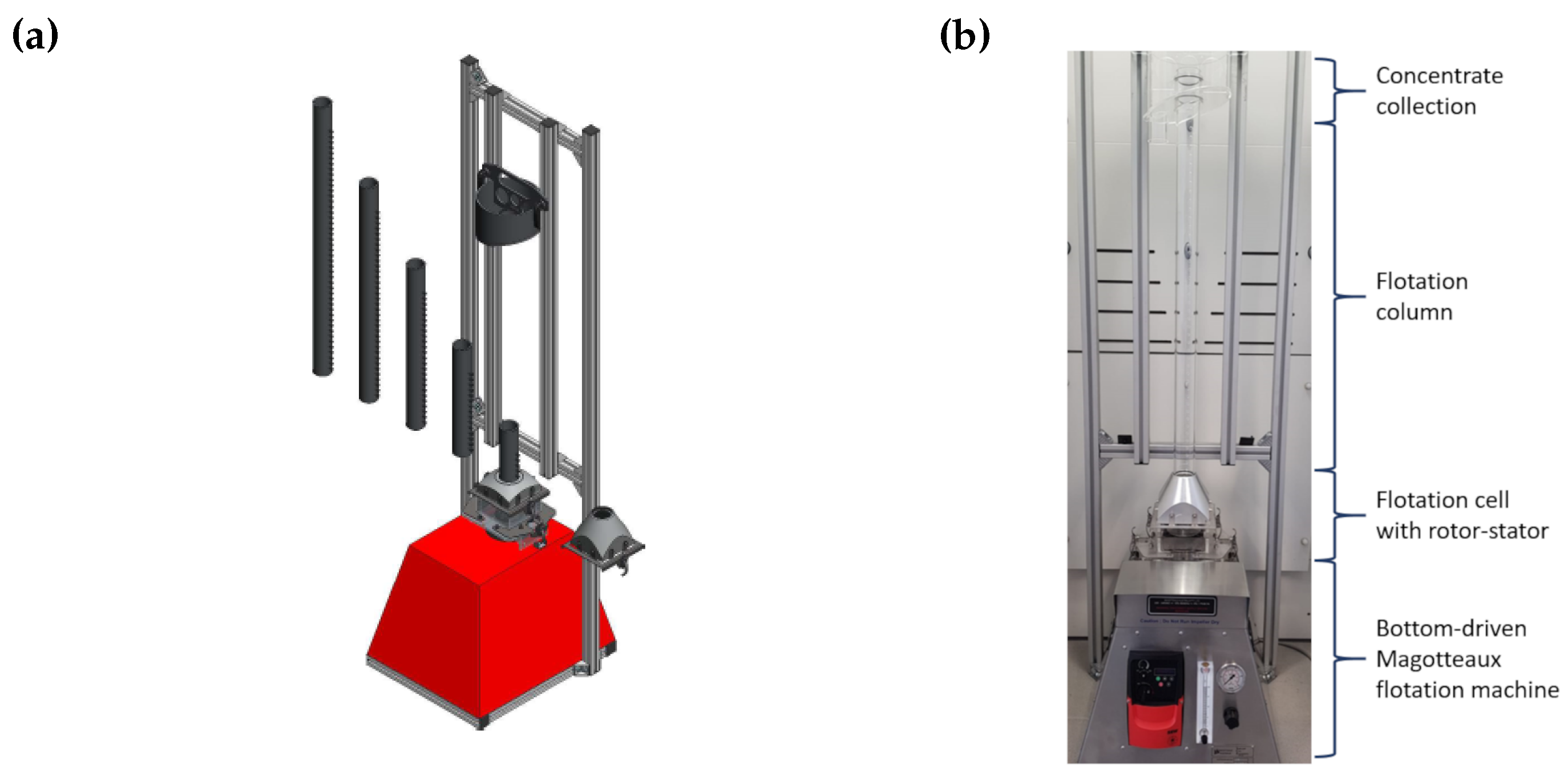
11) if image measurements are available for the concentrate and tailings. However, in practice, MLA measurements of concentrate or tailings are often unavailable or incomplete. For example, in the flotation-based separation process described in Section 2.2 (and analyzed in Section 3.2), the problem arises that the concentrate consists of several fractions of concentrates. Thus, to compute the Tromp function for the complete concentrate (i.e., the union of all single concentrate fractions), all concentrate fractions must be mixed in the measurement process to obtain a single measured fraction for the concentrate. This would lead to a loss of information regarding the individual concentrate fractions. Alternatively, the probability densities of the descriptor vectors of particles in the complete concentrate could be computed as a convex combination of the probability densities of the descriptor vectors of particles in the individual concentrates. However, this method would be rather time consuming because for an increasing number of output fractions, the effort required for MLA measurements and the estimation procedure of the probability densities of particle descriptors for each individual concentrate increases significantly.
Therefore, we present an approach to compute Tromp functions when no measurements are available for some of the separated fractions by solving a minimization problem. In particular, we consider the case when image measurements are available only for feed and tailings, using the probability densities f t and f f instead of f c and f t . To redeem the numerical issues, which can occur when estimating the probability density f f from image measurements as described in Section 2.4.2, we exploit the fact that f f can be expressed as a convex combination of f c and f t , where we replace the (unknown) probability density f c of descriptor vectors associated with particles in the complete concentrate by some parametric approximation f c ˜ : R d [ 0 , ) . More precisely, we assume that f c ˜ is a member of a parametric family { f θ : θ Θ } of multivariate probability densities, e.g., the density of a multivariate normal distribution or a copula-based distribution model as described in Section 2.5, where Θ R d denotes the set of admissible parameters for some integer d 1 . Then, f c ˜ can be determined by solving the following minimization problem:
f c ˜ = arg min θ Θ R d | f f ( x ) ( λ f θ ( x ) + ( 1 λ ) f t ( x ) ) | d x ,
i.e., the function f c ˜ : R d [ 0 , ) minimizes the integral on the right-hand side of Equation (12).
Note that the number-weighted mixing parameter λ in Equation (12) cannot be computed directly if there is no information on the concentrate available. Instead we can determine λ by solving the equation
( 1 λ ) = n t n f .
We also remark that in case of using Equation (12) to obtain an approximation for f c and then computing the Tromp function T utilizing Equation (11), T takes values between zero and one by definition.

2.4.4. Restriction of Tromp Functions

Formally, Tromp functions are defined for all d-dimensional descriptor vectors x R d , see Equations (1) and (11). However, for descriptor vectors x R d such that the corresponding particles are not (or only rarely) observed in the feed, i.e., for which the value of f f ( x ) is equal or close to zero, the value of T ( x ) is not meaningful. Therefore, we present a scheme that constrains the set of admissible particle descriptors for which we compute the separation probability T ( x ) . More precisely, we compute the Tromp function only for descriptor vectors belonging to the set A R d which is given by
A = { x R d : f f ( x ) > ε } ,
where ε = inf s [ 0 , ) : x R d : f f ( x ) s f f ( x ) d x q for some q [ 0 , 1 ] . Note that the threshold q can be used to specify how likely it must be that particles with certain descriptor vectors are observed in the feed for the Tromp function to provide sufficient information about the separation probability of such particles.

2.5. Stochastic Modeling of Particle Descriptor Vectors

In the rest of this paper we mainly focus on the analysis and modeling of two-dimensional particle descriptor vectors x R 2 .
For particles observed in a planar section of a three-dimensional particle system, it is possible to compute various size and shape descriptors using the particle-wise segmentation of 2D images obtained by MLA measurements within some sampling window W Z 2 , see Section 2.3. A question of particular interest is how such particle descriptors can be exploited in order to study the influence of particle morphology on separation processes. Therefore, in Section 2.5.1 we specify a pair of size and shape descriptors which can be easily determined from planar cross sections of particles. Then, in Section 2.5.2, we discuss methods for modeling the distribution of single particle descriptors with univariate probability densities. The parametric copula-based procedure, which is used for modeling the distribution of pairs of such descriptors, is explained in Section 2.5.3. By applying the methods given in Section 2.5.1, Section 2.5.2 and Section 2.5.3 to image data acquired before and after the application of a separation procedure, we can then determine bivariate Tromp functions for characterizing the behavior of separation processes under consideration, see Section 3.

2.5.1. Size and Shape Descriptors

In order to characterize the size of a particle P W observed within the sampling window W R 2 , we determine the area-equivalent diameter of P which is given by
d A ( P ) = 2 A ( P ) π ,
where A ( P ) denotes the area of P . Note that A ( P ) is computed from image data by counting the number of pixels belonging to the correspondingly discretized particle cross-section P W .
Furthermore, we determine the so-called minimum and maximum Feret diameters d min ( P ) and d max ( P ) of P , by deploying the algorithm given in [22]. More precisely, d min ( P ) and d max ( P ) are the smallest and largest edge lengths of a minimum rectangular bounding box B ( x , y , α , β , θ ) of P . Such a bounding box can be determined by solving the minimization problem
( x , y , α , β , θ ) = arg min ( x , y , α , β , θ ) R 4 × [ 0 , π ) , 0 < α β , P B ( x , y , α , β , θ ) α · β ,
where B ( x , y , α , β , θ ) denotes a rectangle with edge lengths 0 < α β which is rotated by θ [ 0 , π ) around its center ( x , y ) R 2 . Then, the minimum and maximum Feret diameters of P are given by d min ( P ) = α and d max ( P ) = β , respectively. This provides the aspect ratio ψ ( P ) of P , which is given by
ψ ( P ) = d min ( P ) d max ( P ) .
Note that the aspect ratio ψ defined in Equation (17) is a shape descriptor which allows us to distinguish between elongated ( ψ ( P ) 1 ) and non-elongated particles ( ψ ( P ) 1 ). Analogously to the computation of the area of a particle cross-section from image data, we compute the minimum and maximum Feret diameters d min ( P ) and d max ( P ) of P by rescaling their values with the pixelsize.

2.5.2. Univariate Stochastic Modeling of Single Particle Descriptors

By computing the size and shape descriptors introduced in Section 2.5.1 for all particles P 1 , , P N W , we obtained a sample of particle descriptor vectors which characterized the particle system observed in the underlying image I : W { 0 , 1 , 2 , } . More precisely, we determined the two-dimensional descriptor vectors x ( 1 ) , , x ( N ) R 2 , where the first entry was the area-equivalent diameter and the second entry was the aspect ratio of the corresponding particle, i.e., x ( i ) = ( d A ( i ) , ψ ( i ) ) for i = 1 , , N .
For each entry of the particle descriptor vectors we fitted a univariate probability density from a parametric family { f θ : θ Θ } of probability densities f θ : R [ 0 , ) (e.g., the densities of normal, log-normal, gamma, or beta distributions), where Θ is the set of admissible parameters, see Table 1. The best fitting density and the corresponding parameters were chosen by means of the maximum-likelihood method [23].
In applications it might be not sufficient to only use parametric families of unimodal probability densities, like those ones mentioned in Table 1. Instead, bimodal densities might provide better fits, which can be achieved by considering convex combinations f θ 1 , θ 2 = w f θ 1 + ( 1 w ) f θ 2 of unimodal probability densities f θ 1 , f θ 2 : R ( 0 , ) for some θ 1 , θ 2 Θ , where w ( 0 , 1 ) is some mixing parameter. However, this increases the number of model parameters. In order to avoid making the model too complex, while increasing the likelihood of the fitted distribution, the best fitting distribution was selected according to the Akaike information criterion [24].

2.5.3. Bivariate Stochastic Modeling of Pairs of Particle Descriptors

The procedure for modeling the distribution of single particle descriptors as stated in Section 2.5.2 does not capture information about the correlation between the descriptors. Therefore, to get a more comprehensive probabilistic characterization of the observed particle system, we fitted a bivariate probability density to the sample of two-dimensional descriptor vectors x ( i ) = ( d A ( i ) , ψ ( i ) ) for i = 1 , , N . For this, we use the fact that each bivariate probability density f : R 2 [ 0 , ) can be represented in the form
f ( x ) = f 1 ( x 1 ) f 2 ( x 2 ) c ( F 1 ( x 1 ) , F 2 ( x 2 ) ) ,
for all x = ( x 1 , x 2 ) R 2 , where f 1 , f 2 : R [ 0 , ) denote the (univariate) marginal densities corresponding to f, i.e., f 1 ( x 1 ) = R f ( x 1 , y 2 ) d y 2 and f 2 ( x 2 ) = R f ( y 1 , x 2 ) d y 1 for all x 1 , x 2 R . Moreover, F 1 , F 2 : R [ 0 , 1 ] are the cumulative distribution functions corresponding to f 1 and f 2 , respectively, and c : [ 0 , 1 ] 2 [ 0 , ) is a bivariate copula density, i.e., a bivariate probability density with uniform marginal distributions on the unit interval [ 0 , 1 ] , see e.g., [18].
Analogously to the situation which has been discussed in Section 2.5.2 for the fitting of univariate probability densities, in the literature various parametric families of bivariate copula densities have been considered. In the present paper, we focus on parametric families of so-called Archimedean copulas, namely Clayton, Frank, Gumbel, and Joe copulas as well as rotated versions of these copula families [18,25], see also Table 2. Then, by means of maximum-likelihood estimation and using the Akaike information criterion, we have determined the best fitting bivariate probability density f : R 2 [ 0 , ) for the sample x ( i ) = ( d A ( i ) , ψ ( i ) ) with i = 1 , , N . See also [17,26], where this approach has been applied for parametric stochastic modeling of similar types of particle-discrete image data.

3. Results

As already mentioned above, wettability properties of particles cannot be observed in MLA data, but the effect of wettability on the separation behavior of particles can be analyzed by comparing multivariate Tromp functions. In this section, bivariate Tromp functions are computed in terms of two particle descriptors: the area-equivalent diameter and the aspect ratio of particles, which can be determined from image data. More precisely, we compute Tromp functions for the flotation-based separation process stated in Section 2.2, which has been performed on two particle systems (spheres and fragments) with three different levels of wettability. Recall that these wettability scenarios are denoted by C 0 , C 6 , and C 10 , respectively. Overall, we analyzed the separation process by computing and analyzing Tromp functions for six different systems of glass particles, where we do not have full information on the concentrate. Thus, in Section 3.1, we present the results which have been obtained for fitting bivariate probability densities to various samples of two-dimensional descriptor vectors of glass particles, exploiting the methods stated in Section 2.5.2 and Section 2.5.3. Then, in Section 3.2, we use the fitted probability densities to compute and analyze the corresponding Tromp functions.

3.1. Fitted Univariate and Bivariate Probability Densities

Recall that by using f f we denote the probability density of descriptor vectors of the glass particles observed in the feed. Furthermore, the probability density of descriptor vectors of particles in the concentrate for unesterified particles will be denoted by f C 0 c , and for the differently modified particles by f C 6 c and f C 10 c . Analogously, let f C 0 t , f C 6 t and f C 10 t denote the corresponding probability densities of particle descriptor vectors in the tailings.
Since for the separation experiments performed in the framework of this paper we do not have full information about the complete concentrate, Tromp functions are computed by means of the minimization procedure stated in Section 2.4.3. For this, we first fit the probability densities f f , f C 0 t , f C 6 t , and f C 10 t of the area-equivalent diameter and aspect ratio of particles observed in the image data for feed and tailings, where we use the parametric (copula-based) distribution models as described in Section 2.5.3, see Table 3 and Table 4.
Recall that, as stated in Section 2.4.2, the probability density f f can be given by
f f ( d A , ψ ) = λ i f C i c ( d A , ψ ) + ( 1 λ i ) f C i t ( d A , ψ ) ,
for all pairs ( d A , ψ ) [ 0 , ) × [ 0 , 1 ] and for each i { 0 , 6 , 10 } , where λ i is the mixing parameter corresponding to the wettability scenario C i , given as the number of particles in the complete concentrate divided by the number of particles in the feed. The numbers of particles observed in the image data of feed and tailings for glass spheres and fragments and for the wettability scenarios C 0 , C 6 and C 10 are presented in Table 5, where the number of particles in the complete concentrate has been determined by means of Equation (13).
From a formal point of view, the probability densities f f , f C 0 t , f C 6 t and f C 10 t could be computed first from image data and then used to approximately obtain f C 0 c , f C 6 c , and f C 10 c by means of Equation (12). However, this would have the disadvantage that the validity of Equation (19) would be violated in the sense that, in general, its right-hand side and, therefore, also its left-hand side would depend on i { 0 , 6 , 10 } .
To overcome this issue, we only compute the density f C 0 c as suggested in Section 2.4.3 by solving the minimization problem stated in Equation (12), see Table 6. For this, we use the densities f f and f C 0 t which are obtained from fitting parametric models to the descriptor vectors extracted from image data for feed and tailings, respectively, where we assume that the objective function of the minimization problem considered in Equation (12) is from the same family of parametric distributions as the density f f fitted from image data.
Afterwards we re-compute f f for the experiment C 0 with unesterified particles by means of Equation (19) for i = 0 . The probability density f f obtained in this way is then used to determine f C 6 c and f C 10 c by solving the equation
λ C 0 f C 0 c ( d A , ψ ) + ( 1 λ C 0 ) f C 0 t ( d A , ψ ) = λ C i f C i c ( d A , ψ ) + ( 1 λ C i ) f C i t ( d A , ψ ) ,
for all pairs ( d A , ψ ) [ 0 , ) × [ 0 , 1 ] and for each i { 6 , 10 } . Thus, the probability densities f C 6 c and f C 10 c are given by
f C i c ( d A , ψ ) = λ C 0 f C 0 c ( d A , ψ ) + ( 1 λ C 0 ) f C 0 t ( d A , ψ ) ( 1 λ C i ) f C i t ( d A , ψ ) λ C i ,
for all ( d A , ψ ) [ 0 , ) × [ 0 , 1 ] and i { 6 , 10 } .
The algorithm stated above is motivated by the fact that for each of the two morphological particle scenarios considered in this paper (i.e., for spheres and fragments, respectively) the same feed material is used for the thee wettability scenarios C 0 , C 6 , and C 10 . Furthermore, the reason for re-computing the density f f for unesterified particles by means of Equation (19) is that in this case the largest number of glass particles has been observed in image measurements for the tailings, see Table 5.
In addition, all fitted probability densities are truncated such that only particles with an area-equivalent diameter and an aspect ratio above and below certain thresholds are taken into consideration. In this way, we have improved the goodness of the fit of the parametric models described above. In particular, we have truncated the probability densities of the area-equivalent diameter of glass spheres to the interval [ 2 , 10 ] μ m , and those of glass fragments to [ 2 , 8 ] μ m , where the lower threshold results from the resolution limit of MLA measurements and only very few outliers of particles of both particle systems are observed with an area-equivalent diameter larger than the corresponding upper threshold. Analogously, we truncate the probability densities of the aspect ratio for both particle systems to the interval [ 0.2 , 1 ] , since no particles with an aspect ratio smaller than 0.2 are observed in the MLA measurements.

3.2. Computed Bivariate Tromp Functions

Using the probability densities stated in Section 3.1, bivariate Tromp functions are computed by means of Equation (11). In Figure 4, the Tromp functions are visualized which have been obtained for spherical (upper row) and fractured glass particles (lower row), respectively, and for unesterified (left column) as well as for esterified particles of the wettability scenarios C 6 (middle column) and C 10 (right column). The bright yellow color indicates that particles in the feed with corresponding area-equivalent diameter and aspect ratio are more likely to be separated into the concentrate, while the dark blue color indicates that a particle with the corresponding descriptor vector is separated into the tailings.
Note that in order to obtain a more meaningful interpretation for the probability that a particle is separated into the concentrate or the tailings, we computed the Tromp functions only for pairs ( d A , ψ ) of descriptor vectors belonging to the set A R 2 given in Equation (14), where we put q = 0.01 , i.e., we computed the Tromp functions only for pairs of descriptor vectors corresponding to particles which are likely to be observed in the feed. The set of pairs ( d A , ψ ) corresponding to particles which are not observed with sufficiently high frequency in the feed, i.e., ( d A , ψ ) A , are indicated in the white color in Figure 4.
A quantitative analysis of the changes of Tromp functions shown in Figure 4, when passing from left to right columns, was performed by computing the point-wise differences between the values of the Tromp functions obtained for the experiments with esterified particles and those obtained for unesterified particles. More precisely, for each particle system (spheres, fragments), from the Tromp functions obtained for the wettability scenarios C 6 and C 10 , respectively, the Tromp function obtained for C 0 is subtracted, see Figure 5.
Furthermore, the Tromp functions shown in Figure 4 can be used in order to analyze the separation uncertainty of the flotation-based separation process considered in the present paper. For this purpose, for separation processes producing two output fractions, the Shannon entropy function H : A [ 0 , 1 ] were considered [13,27], which is given by
H ( d A , ψ ) = T ( d A , ψ ) log 2 ( T ( d A , ψ ) ) + T t ( d A , ψ ) log 2 ( T t ( d A , ψ ) ) ,
for all pairs ( d A , ψ ) A , where log 2 denotes the logarithm to the basis 2 (i.e., s = 2 log 2 ( s ) for all s > 0 ), and T t ( d A , ψ ) = 1 T ( d A , ψ ) can be interpreted as the probability that a particle with particle descriptor vector ( d A , ψ ) A is separated into the tailings, see Figure 6.
The values H ( d A , ψ ) of the entropy function given in Equation (22) can be interpreted as follows. For pairs ( d A , ψ ) of descriptors for which H ( d A , ψ ) is close to zero, there is a low uncertainty in the separation process, i.e., particles with such descriptor vectors have a separation probability close to zero or one, which means that such particles are separated with high probability, either into the concentrate or the tailings. On the other hand, if H ( d A , ψ ) is close to one, the separation probability is close to 0.5 and thus, it is uncertain whether such a particle is separated into the concentrate or the tailings.
Moreover, the mean entropy given by H ¯ = A H ( d A , ψ ) d ( d A , ψ ) can be used to compare the uncertainty of different separation experiments for a given feed composition (e.g., spherical or fragmented glass particles with magnetite), see Table 7. In this way, it is possible to analyze the influence of changes in particle wettability on the separation uncertainty.

4. Discussion

As shown in the previous section, the differently shaped white areas in the upper and lower rows of Figure 4 indicate significant differences in size and shape of the two systems of glass particles. The spheres have larger area-equivalent diameters and, not surprisingly, larger aspect ratios than the fragments. Furthermore, it has been shown that for unesterified glass spheres ( C 0 ) the area-equivalent diameter does not influence the separation behavior significantly and mainly the aspect ratio is the dominating particle descriptor since all size fractions are recovered in the concentrate as long as the particles have an aspect ratio of around 0.8–1.0. If the wettability is now modified and the spheres are strongly hydrophobic ( C 10 ), the significance of the individual particle descriptors of size and shape have less impact on the separation behavior, since most of the particles (except for particles with an area-equivalent diameter of about 6–8 μ m and an aspect ratio of about 0.4–0.9) were recovered in the concentrate and the wettability was the dominating separation property. In the case of glass fragments a different outcome has been observed. The results of the Tromp functions for fragments with wettability states of C 0 and C 6 showed that mostly very fine particles with varying aspect ratios were recovered in the concentrate. An increase in hydrophobicity ( C 10 ) resulted in a higher probability of recovering particles with a slightly larger area-equivalent diameter, while the aspect ratio still showed no significant influence.
Looking at the point-wise differences of the Tromp functions for esterified particles in comparison to the Tromp functions for unesterified particles in Figure 5, the changes of Tromp functions when passing to the wettability scenario C 10 have become even more apparent. While the point-wise differences of Tromp functions for spherical particles show larger positive and negative variations, the values of Tromp functions for glass fragments changed only slightly when passing from unesterified particles to esterified particles of wettability scenario C 6 . On the other hand, the Tromp functions for fragments changed much more when passing to C 10 , in particular for particles with a larger area-equivalent diameter. Note that when the particles became more hydrophobic, fewer glass particles were observed in the tailings, see Table 5, i.e., more glass particles were separated into the concentrate.
For spherical particles, the separation uncertainty expressed by the entropy functions in the upper rows of Figure 6 was close to zero for particles with a large aspect ratio ( ψ > 0.8 ), independent of their area-equivalent diameter and for all wetting scenarios. For particles with a smaller aspect ratio, the separation uncertainty decreased with increasing hydrophobicity of the particles. The values of mean entropy given in the middle column of Table 7 for spheres confirmed the trend of globally decreasing separation uncertainty with increasing hydrophobicity of spherical particles. In contrast to this, the mean separation uncertainty did not change significantly for fragmented glass particles when passing from unesterified particles to the wettability scenarios C 6 and C 10 , see Table 7. On the other hand, we observed that the entropy values H ( d A , ψ ) for given pairs ( d A , ψ ) of fragment descriptors differed locally for different wettability scenarios; see the lower row of Figure 6. For unesterified particles with area-equivalent diameters larger than 4   μ m the entropy values H ( d A , ψ ) were small, while for the wettability scenarios C 6 and C 10 the entropy values H ( d A , ψ ) were larger for particles with the same sizes, i.e., the separation uncertainty increased. Thus, it is not sufficient to limit ourselves to the investigation of mean entropy when analyzing the separation uncertainty. Furthermore, the different behavior of the separation uncertainty of the two particle systems (spheres, fragments) showed that the separation process was influenced differently by the wettability for different particle morphologies.
It should be noted that the particle descriptors being used in this study may not accurately represent the true 3D structure of the glass particles due to certain effects being not observable in 2D image data obtained by MLA. For example, a reason for this can be that the aspect ratio of some particles can vary greatly depending on the angle of the image capture, resulting in a potential bias for aspect ratio distributions determined from 2D data. However, despite this limitation, these descriptors still allowed some level of quantitative structural evaluation of the impact of particle morphology and wettability on separation behavior.
Furthermore, the results obtained by the optimization procedure proposed in Section 2.4.3 depended on the accuracy of the probability densities f f , f C 0 t , f C 6 t and f C 10 t computed from image data of the feed and tailings. Since we computed Tromp functions for particles which were mainly enriched into the concentrate, this suggests that the accuracy of the computed Tromp functions might be further improved by performing image measurements of feed and concentrate instead of feed and tailings. In this way, we could obtain a better fit of the required probability densities computed directly from image data and, thus, gain more accurate results for corresponding Tromp functions, while maintaining the advantages of the optimization procedure of Section 2.4.3 for reducing the measurement effort.

5. Conclusions

The analysis of bivariate Tromp functions performed in the present paper provides an innovative approach for the multidimensional evaluation of the combined influence of factors like particle wettability, morphology and size on the flotation-based separation behavior. We proposed a parametric modeling approach in order to determine the Tromp functions from image data, which have been gained by scanning electron microscopy measurements for the feed and separated fractions. The underlying bivariate probability densities of particle descriptor vectors have been fitted to data by utilizing Archimedean copulas. We extended this modeling approach by an optimization routine in order to analyze the behavior of separation processes also in the case when image measurements are not available for all separated fractions. Furthermore, the Tromp functions have been used in order to analyze the separation uncertainty of the flotation-based separation process, where the Shannon entropy function is considered.

Author Contributions

Conceptualization, M.R. and V.S.; methodology, T.W., J.S. and O.F.; software, T.W.; data curation, J.S. and K.B.; writing—original draft preparation, T.W., J.S. and O.F.; writing—review and editing, T.W., J.S., O.F., K.B., M.R. and V.S.; visualization, T.W.; supervision, M.R. and V.S.; project administration, M.R. and V.S.; funding acquisition, M.R. and V.S. All authors have read and agreed to the published version of the manuscript.

Funding

This research is partially funded by the German Research Foundation (DFG) via the research projects RU2184/1-2, SCHM997/27-2 and SCHM997/45-1 within the priority programs SPP 2045 “Highly specific and multidimensional fractionation of fine particle systems with technical relevance” and SPP 2315 “Engineered artificial minerals (EnAM)— A geo-metallurgical tool to recycle critical elements from waste streams”.

Data Availability Statement

The datasets generated and/or analyzed during the current study are available from the corresponding author on reasonable request.

Conflicts of Interest

The authors declare no conflict of interest and the funders had no role in the design of the study; in the collection, analyses, or interpretation of data; in the writing of the manuscript; or in the decision to publish the results.

References

  1. Koh, P.T.L.; Hao, F.P.; Smith, L.K.; Chau, T.T.; Bruckard, W.J. The effect of particle shape and hydrophobicity in flotation. Int. J. Miner. Process. 2009, 93, 128–134. [Google Scholar] [CrossRef]
  2. Hassas, B.V.; Caliskan, H.; Guven, O.; Karakas, F.; Cinar, M.; Celik, M.S. Effect of roughness and shape factor on flotation characteristics of glass beads. Colloids Surfaces A Physicochem. Eng. Asp. 2016, 492, 88–99. [Google Scholar] [CrossRef]
  3. Verrelli, D.I.; Bruckard, W.J.; Koh, P.T.L.; Schwarz, M.P.; Follink, B. Particle shape effects in flotation. Part 1: Microscale experimental observations. Miner. Eng. 2014, 58, 80–89. [Google Scholar] [CrossRef]
  4. Xia, W. Role of particle shape in the floatability of mineral particle: An overview of recent advances. Powder Technol. 2017, 317, 104–116. [Google Scholar] [CrossRef]
  5. Chen, Y.; Zhuang, L.; Zhang, Z. Effect of particle shape on particle-bubble interaction behavior: A computational study using discrete element method. Colloids Surfaces A Physicochem. Eng. Asp. 2022, 653, 130003. [Google Scholar] [CrossRef]
  6. Little, L.; Wiese, J.; Becker, M.; Mainza, A.; Ross, V. Investigating the effects of particle shape on chromite entrainment at a platinum concentrator. Miner. Eng. 2016, 96-97, 46–52. [Google Scholar] [CrossRef]
  7. Wiese, J.; Becker, M.; Yorath, G.; O’Connor, C. An investigation into the relationship between particle shape and entrainment. Miner. Eng. 2015, 83, 211–216. [Google Scholar] [CrossRef]
  8. Kupka, N.; Tolosana-Delgado, R.; Schach, E.; Bachmann, K.; Heinig, T.; Rudolph, M. R as an environment for data mining of process mineralogy data: A case study of an industrial rougher flotation bank. Miner. Eng. 2020, 146, 106111. [Google Scholar] [CrossRef]
  9. Schubert, H. On the optimization of hydrodynamics in fine particle flotation. Miner. Eng. 2008, 21, 930–936. [Google Scholar] [CrossRef]
  10. Trahar, W.J.; Warren, L.J. The flotability of very fine particles—A review. Int. J. Miner. Process. 1976, 3, 103–131. [Google Scholar] [CrossRef]
  11. Miettinen, T.; Ralston, J.; Fornasiero, D. The limits of fine particle flotation. Miner. Eng. 2010, 23, 420–437. [Google Scholar] [CrossRef]
  12. Wang, L.; Peng, Y.; Runge, K.; Bradshaw, D. A review of entrainment: Mechanisms, contributing factors and modelling in flotation. Miner. Eng. 2015, 70, 77–91. [Google Scholar] [CrossRef]
  13. Schach, E.; Buchmann, M.; Tolosana-Delgado, R.; Leißner, T.; Kern, M.; van den Boogaart, K.G.; Rudolph, M.; Peuker, U.A. Multidimensional characterization of separation processes—Part 1: Introducing kernel methods and entropy in the context of mineral processing using SEM-based image analysis. Miner. Eng. 2019, 137, 78–86. [Google Scholar] [CrossRef]
  14. Leißner, T.; Bachmann, K.; Gutzmer, J.; Peuker, U.A. MLA-based partition curves for magnetic separation. Miner. Eng. 2016, 94, 94–103. [Google Scholar] [CrossRef]
  15. Buchmann, M.; Schach, E.; Tolosana-Delgado, R.; Leißner, T.; Astoveza, J.; Möckel, R.; Ebert, D.; Rudolph, M.; von de Boogaart, K.G.; Peuker, U.A. Evaluation of magnetic separation efficiency on a Cassiterite-Bearing Skarn ore by means of integrative SEM-based image and XRF–XRD data analysis. Minerals 2018, 8, 390. [Google Scholar] [CrossRef]
  16. Scott, D.W. Multivariate Density Estimation: Theory, Practice, and Visualization; John Wiley & Sons: Hoboken, NJ, USA, 2015. [Google Scholar]
  17. Furat, O.; Leißner, T.; Bachmann, K.; Gutzmer, J.; Peuker, U.A.; Schmidt, V. Stochastic modeling of multidimensional particle characteristics using parametric copulas. Microsc. Microanal. 2019, 25, 720–734. [Google Scholar] [CrossRef]
  18. Nelsen, R. An Introduction to Copulas; Springer: Berlin/Heidelberg, Germany, 2006. [Google Scholar]
  19. Sygusch, J.; Rudolph, M. A contribution to wettability and wetting characterisation of ultrafine particles with varying shape and degree of hydrophobization. Appl. Surf. Sci. 2021, 566, 150725. [Google Scholar] [CrossRef]
  20. Furat, O.; Masuhr, M.; Kruis, F.E.; Schmidt, V. Stochastic modeling of classifying aerodynamic lenses for separation of airborne particles by material and size. Adv. Powder Technol. 2020, 31, 2215–2226. [Google Scholar] [CrossRef]
  21. Frank, U.; Wawra, S.E.; Pflug, L.; Peukert, W. Multidimensional particle size distributions and their application to nonspherical particle systems in two dimensions. Part. Part. Syst. Charact. 2019, 36, 1800554. [Google Scholar] [CrossRef]
  22. VolkerH/feret_diameter.py. Available online: https://gist.github.com/VolkerH/0d07d05d5cb189b56362e8ee41882abf (accessed on 16 August 2022).
  23. Held, L.; Bové, D.S. Applied Statistical Inference: Likelihood and Bayes; Springer: Berlin/Heidelberg, Germany, 2014. [Google Scholar]
  24. Akaike, H. Information theory and an extension of the maximum likelihood principle. In Selected Papers of Hirotugu Akaike; Springer: Berlin/Heidelberg, Germany, 1998; pp. 199–213. [Google Scholar]
  25. Joe, H. Dependence Modeling with Copulas; CRC Press: Boca Raton, FL, USA, 2014. [Google Scholar]
  26. Ditscherlein, R.; Furat, O.; de Langlard, M.; de Souza e Silva, J.M.; Sygusch, J.; Rudolph, M.; Leißner, T.; Schmidt, V.; Peuker, U.A. Multi-scale tomographic analysis for micron-sized particulate samples. Microsc. Microanal. 2020, 26, 676–688. [Google Scholar] [CrossRef]
  27. Buchmann, M.; Schach, E.; Leißner, T.; Kern, M.; Mütze, T.; Rudolph, M.; Peuker, U.A.; Tolosana-Delgado, R. Multidimensional characterization of separation processes – Part 2: Comparability of separation efficiency. Miner. Eng. 2020, 150, 106284. [Google Scholar] [CrossRef]
Figure 1. SEM images of the floatable fractions of glass spheres (a) and glass fragments (b), and the non-floatable fraction of magnetite (c); the corresponding particle-size probability density of volume-equivalent diameter obtained by laser diffraction (d).
Powders 02 00021 g001
Figure 2. Contact angles of the pristine glass slides ( C 0 ) and those esterified with 1-hexanol ( C 6 ) and 1-decanol ( C 10 ) measured in sessile drop mode via optical contour analysis. The glass slides have the same chemical composition as the glass particles used in this study and were cleaned and esterified in the same way as the glass particles.
Powders 02 00021 g002
Figure 3. Schematic drawing of the MultiDimFlot separation apparatus (a) and its implementation in the lab (b).
Powders 02 00021 g003
Figure 4. Bivariate Tromp functions for spherical (upper row) and fragmented (lower row) glass particles, and for unesterified particles (left column) as well as for particles with differently modified levels of hydrophobicity by esterification corresponding to the wettability scenarios C 6 (middle column) and C 10 (right column).
Powders 02 00021 g004
Figure 5. Point-wise differences between Tromp functions for spherical (upper row) and fragmented (lower row) particles, where the Tromp functions obtained for the wettability scenarios C 6 (left column) and C 10 (right column) are subtracted from the Tromp function obtained for C 0 .
Powders 02 00021 g005
Figure 6. Bivariate entropy functions for spherical (upper row) and fragmented (lower row) glass particles, and for unesterified particles (left column) as well as for particles with differently modified levels of hydrophobicity by esterification corresponding to the wettability scenarios C 6 (middle column) and C 10 (right column).
Powders 02 00021 g006
Table 1. Parametric families of univariate distributions used in Section 3.1 for fitting the marginal probability densities of the bivariate probability densities f f , f c and f t .
Parametric FamilyProbability Density
Normal f θ ( x ) = 1 2 π σ 2 e ( x μ ) 2 2 σ 2 , θ = ( μ , σ ) R × ( 0 , )
Log-normal f θ ( x ) = 1 2 π σ 2 x 2 e ( log ( x ) log ( μ ) ) 2 2 σ 2 𝟙 ( 0 , ) ( x ) , θ = ( μ , σ ) R × ( 0 , )
Gamma f θ ( x ) = 1 b k Γ ( k ) x k 1 e x b 𝟙 ( 0 , ) ( x ) , θ = ( k , b ) ( 0 , ) 2
Beta f θ ( x ) = Γ ( α + β ) Γ ( α ) Γ ( β ) x α 1 ( 1 x ) β 1 𝟙 ( 0 , 1 ) ( x ) , θ = ( α , β ) ( 0 , ) 2
Table 2. Parametric copula families used in Section 3.1 for fitting the bivariate densities f f , f c , and f t .
Parametric FamilyCopula Density
Clayton c θ ( u 1 , u 2 ) = ( θ + 1 ) ( u 1 u 2 ) ( θ 1 ) ( u 1 θ + u 2 θ 1 ) 2 θ + 1 θ , θ ( 0 , )
Frank c θ ( u 1 , u 2 ) = θ ( 1 e θ ) e θ ( u 1 + u 2 ) 1 e θ ( 1 e θ u 1 ) ( 1 e θ u 2 ) , θ ( 0 , )
Gumbel c θ ( u 1 , u 2 ) = 2 u 1 u 2 e ( ( log ( u 1 ) ) θ + ( log ( u 2 ) ) θ ) 1 θ , θ ( 1 , )
Table 3. Bivariate probability density f f fitted to samples of descriptor vectors from image data. The subscript of the parameters indicates whether the parameter corresponds to the first or second probability density of the mixture of univariate probability densities.
Type of ParticlesDescriptorParametric Family of Distributions/CopulasFitted Parameter Values
d A Log-normal-Log-normal mixture μ 1 = 2.54 , σ 1 = 0.13 , μ 2 = 3.58 , σ 2 = 0.22 , w = 0.25
Spheres ψ Normal-Normal mixture μ 1 = 0.89 , σ 1 = 0.04 , μ 2 = 0.62 , σ 2 = 0.15 , w = 0.70
( d A , ψ ) Gumbel θ = 1.36
d A Log-normal-Log-normal mixture μ 1 = 2.18 , σ 1 = 0.05 , μ 2 = 2.74 , σ 2 = 0.15 , w = 0.31
Fragments ψ Normal-Normal mixture μ 1 = 0.62 , σ 1 = 0.13 , μ 2 = 0.86 , σ 2 = 0.04 , w = 0.89
( d A , ψ ) Frank θ = 0.55
Table 4. Bivariate probability densities f C 0 t , f C 6 t and f C 10 t fitted to samples of descriptor vectors from image data. The subscript of the parameters indicates whether the parameter corresponds to the first or second probability density of the mixture of univariate probability densities.
Type of ParticlesEsterificationDescriptorParametric Family of Distributions/CopulasFitted Parameter Values
d A Gamma-Log-normal mixture k = 81.91 , b = 0.03 , μ = 3.51 , σ = 0.25 , w = 0.22
C 0 ψ Normal-Normal mixture μ 1 = 0.58 , σ 1 = 0.12 , μ 2 = 0.82 , σ 2 = 0.06 , w = 0.71
( d A , ψ ) Clayton θ = 0.09
d A Log-normal-Normal mixture μ 1 = 0.24 , σ 2 = 3.11 , μ 2 = 5.62 , σ 2 = 1.67 , w = 0.93
Spheres C 6 ψ Normal-Normal mixture μ 1 = 0.77 , σ 2 = 0.09 , μ 2 = 0.54 , σ 2 = 0.10 , w = 0.44
( d A , ψ ) Clayton θ = 0.07
d A Log-normal-Log-normal mixture μ 1 = 0.22 , σ 2 = 2.96 , μ 2 = 0.26 , σ 2 = 5.64 , w = 0.84
C 10 ψ Beta α = 7.23 , β = 4.47
( d A , ψ ) Frank θ = 0.99
d A Log-normal-Log-normal mixture μ 1 = 2.51 , σ 1 = 0.14 , μ 2 = 3.88 , σ 2 = 0.27 , w = 0.32
C 0 ψ Normal-Normal mixture μ 1 = 0.76 , σ 1 = 0.09 , μ 2 = 0.55 , σ 2 = 0.11 , w = 0.38
( d A , ψ ) Frank θ = 0.82
d A Log-normal-Log-normal mixture μ 1 = 2.43 , σ 1 = 0.12 , μ 2 = 3.85 , σ 2 = 0.27 , w = 0.28
Fragments C 6 ψ Normal-Normal mixture μ 1 = 0.78 , σ 1 = 0.08 , μ 2 = 0.55 , σ 2 = 0.11 , w = 0.34
( d A , ψ ) Frank θ = 0.78
d A Log-normal-Log-normal mixture μ 1 = 4.00 , σ 1 = 0.26 , μ 2 = 2.58 , σ 2 = 0.15 , w = 0.62
C 10 ψ Normal-Normal mixture μ 1 = 0.75 , σ 1 = 0.09 , μ 2 = 0.52 , σ 2 = 0.10 , w = 0.43
( d A , ψ ) Frank θ = 1.00
Table 5. Number of glass particles in feed, tailings and complete concentrate.
FeedTailingsConcentrate
Esterification C 0 C 6 C 10 C 0 C 6 C 10
Spheres 69,762 34921371486 66,270 68,391 69,276
Fragments 19,851 427535071417 15,576 16,344 18,434
Table 6. Bivariate probability density f C 0 c computed by solving the optimization problem given in Equation (12). The subscript of the parameters indicates whether the parameter corresponds to the first or second probability density of the mixture of univariate probability densities.
Glass ParticlesDescriptorsFamily of Distributions/
Copula Families
Fitted Parameter Values
d A Log-normal-Log-normal mixture μ 1 = 2.55 , σ 1 = 0.13 , μ 2 = 3.58 , σ 2 = 0.22 , w = 0.25
Spheres ψ Normal-Normal mixture μ 1 = 0.89 , σ 1 = 0.03 , μ 2 = 0.62 , σ 2 = 0.14 , w = 0.73
( d A , ψ ) Gumbel θ = 1.38
d A Log-normal-Log-normal mixture μ 1 = 2.19 , σ 1 = 0.05 , μ 2 = 2.74 , σ 2 = 0.12 , w = 0.37
Fragments ψ Normal-Normal mixture μ 1 = 0.62 , σ 1 = 0.12 , μ 2 = 0.86 , σ 2 = 0.04 , w = 0.89
( d A , ψ ) Frank θ = 1.00
Table 7. Mean entropy of the flotation-based separation process for various experimental setups, which have been performed for two different particle systems (spheres and fragments) with differently modified wettability scenarios ( C 0 , C 6 and C 10 ).
Wettability ScenarioSpheresFragments
C 0 0.61 0.54
C 6 0.36 0.63
C 10 0.28 0.51
Disclaimer/Publisher’s Note: The statements, opinions and data contained in all publications are solely those of the individual author(s) and contributor(s) and not of MDPI and/or the editor(s). MDPI and/or the editor(s) disclaim responsibility for any injury to people or property resulting from any ideas, methods, instructions or products referred to in the content.

