Acoustic Sensing and Supervised Machine Learning for In Situ Classification of Semi-Autogenous (SAG) Mill Feed Size Fractions Using Different Feature Extraction Techniques

Highlights

What are the main findings?

• Laboratory SAG mill acoustics are sensitive to different feed size fractions.
• Supervised classification models and acoustic emissions were suitable for predicting different feed size fractions in laboratory SAG mills.

What is the implication of the main finding?

• SAG mill acoustics can serve as online proxy tool for providing more insight into different feed size fractions in the mill.
• The practical implication of the study could be beneficial to SAG mill operators by predicting a sudden change in feed size in real-time.

Abstract

The harsh and hostile internal environment of semi-autogenous (SAG) mills renders real-time monitoring of some critical variables practically unmeasured. Typically, feed size fractions are known to cause mill fluctuations and impede the consistent processing behaviour of ores. There is, therefore, the need for continuous monitoring of mill parameters for optimal operation. In this paper, an acoustic-based sensing method is employed to estimate, in real time, a snapshot of the different feed size fractions presented to a laboratory-scale SAG mill. Employing the MATLAB 2020b programme, the mill acoustic signal is processed using various transform techniques such as power spectral density estimate (PSDE) by Welch’s method, discrete wavelet transform (DWT), wavelet packet transform (WPT), empirical mode decomposition (EMD), and variational mode decomposition (VMD). Different fractional bandpowers are obtained from the PSDE spectrum, while the statistical root mean square values are further extracted from DWT, WPT, EMD, and VMD as feature vectors. The features are used as input features in different machine-learning classification algorithms for different mill feed size fractions predictions. The various transform techniques and feed size fraction predictions are evaluated using the various performance indicators obtained from the confusion matrix such as accuracy, precision, sensitivity and F1 score. The study showed that the acoustic signal feature extraction techniques used in conjunction with the Support Vector Machine (SVM), linear discriminant analysis (LDA), and ensemble with subclass discriminant machine learning algorithms demonstrated improved performance for predicting feed size variations.

1. Introduction

The operations of AG/SAG mills are known to be sensitive to the changes in feed particle size distributions presented to the mill [1]. The variation of feed particle size significantly affects the overall process control, product quality, and economic performance of the mill [2,3,4]. Poor product quality from the AG/SAG mill poses significant challenges to downstream processes such as flotation, pre-treatment, leaching and dewatering [5,6,7,8,9,10]. As high-grade and easy-to-access ores (surface mining ores) continue to decline, miners have turned to deep pits for ores, which have a high degree of ore hardness. The changes in the ore hardness, coupled with sophisticated mining methods, subsequently define the feed size ranges introduced into the AG/SAG mill. The internal workings of an AG/SAG mill are difficult to visualise and capture in real time because the shell of the mill is opaque, and the grinding environment is aggressive [11,12,13,14]. Several methods have been adopted to understand and control the feed particle size distribution before feeding the SAG mill aimed at improving process stability [3]. These methods have demonstrated some level of success, but more advanced approaches are still required to improve control efficiency. Real-time monitoring of the feed size variations in the mill could be an important tool to optimize mill performance [14].

Advanced control techniques are an exciting development by which mining companies can improve and optimise SAG mill grinding performances via real-time monitoring technology [15]. In addition, the measurement of vibration-acoustic emission signals has emerged as a promising tool to understand the state of the mill (AG/SAG mill and ball mills) [16,17,18,19,20,21,22,23,24,25,26,27,28]. Notwithstanding, more accurate and precise prediction is a topical subject and of great interest to mineral processing engineers for monitoring mill parameters (e.g., feed size distribution) as a pathway to mitigate mill disturbances. The development of such methods can be employed in comminution to provide mill operators with quick decision-making information; for example, in the event of sudden fluctuations in feed size distribution due to failure of upstream measures such as crusher wear and screen damage.

The advent of machine-learning algorithms (supervised and non-supervised learning) has gained frontline attention in many areas, including AG/SAG mills as they offer several advantages in solving complex problems [29,30,31]. Common machine-learning (supervised learning) algorithms employed in this quest include the Support Vector Machine (SVM), Decision Tree (DT), Random Forest (RF), and Artificial Neural Networks (ANN) [32]. Machine learning, in combination with vibration or acoustic emissions, has been reported as an innovative and successful approach for handling complex and dynamic systems such as AG/SAG mills [30]. In a study by Nayak et al. (2020), the prediction of the fill level of a ball mill was performed using different transforms deduced from vibration signals and the ANN algorithm. The outcome of the study showed that features derived from fast Fourier transform (FFT) and ANN algorithm were the most suitable for predicting different fill levels in a ball mill. Another study by Li et al. (2021) used mill acoustic emissions generated from DEM simulations and the ANN model to predict the particle flow dynamics, such as particle size distribution, the mill filling level (throughput), and the energy distribution of a ball mill [33]. Spencer and Sharp (2006) employed the principal component analysis (PCA) and hierarchical clustering (unsupervised machine learning) together with AG/SAG mill surface vibration to develop robust models for mill charge, feed and charge size, pulp density, and feed rate [14]. Zeng and Forssberg (1994) used ball mill vibration-acoustic signal and PCA to develop multiple regression models for monitoring process variables, such as feed rate, pulp density feed size, product size, and power draw [34]. According to the study’s findings, the product size and power draw are largely linked to the vibration signal, while the other parameters are to the acoustic signal. Furthermore, Zeng and Forssberg (1996) used PCA in conjunction with vibration signals to investigate the breakage characteristics of mono-size feed particles in a hydraulic press machine [23]. However, studies on the conjoint use of machine-learning techniques and acoustic sensing for predicting different feed size distributions in an AG/SAG mill are limited.

The current study seeks to combine mill acoustic emission responses and supervised machine learning (classification algorithms) to predict different feed size fractions inside AG/SAG mill operations in real time. The acoustic emission responses of nine different feed size distributions in a purpose-built laboratory AG/SAG mill were measured using an acoustic sensor. Different acoustic signal processing techniques or transforms, such as power spectral density estimate (PSDE), discrete wavelet transform (DWT), wavelet packet transform (WPT), empirical mode decomposition (EMD), and variational mode decomposition (VMD), coupled with the statistical root mean square (RMS), were subjected to six standard classification algorithms. The following key research questions were addressed accordingly:

(a)

Which statistical features can best describe acoustic signal variations?

(b)

What is the response of varying AG/SAG mill feed size fractions in terms of acoustic emission?

(c)

What are the performances of the various extraction techniques used in the study for predicting different feed size distributions inside the laboratory-scale AG/SAG mill?

(d)

Which signal extraction technique and classification can best predict different feed size fractions within the mill?

(e)

What is the overall practical overview of the study?

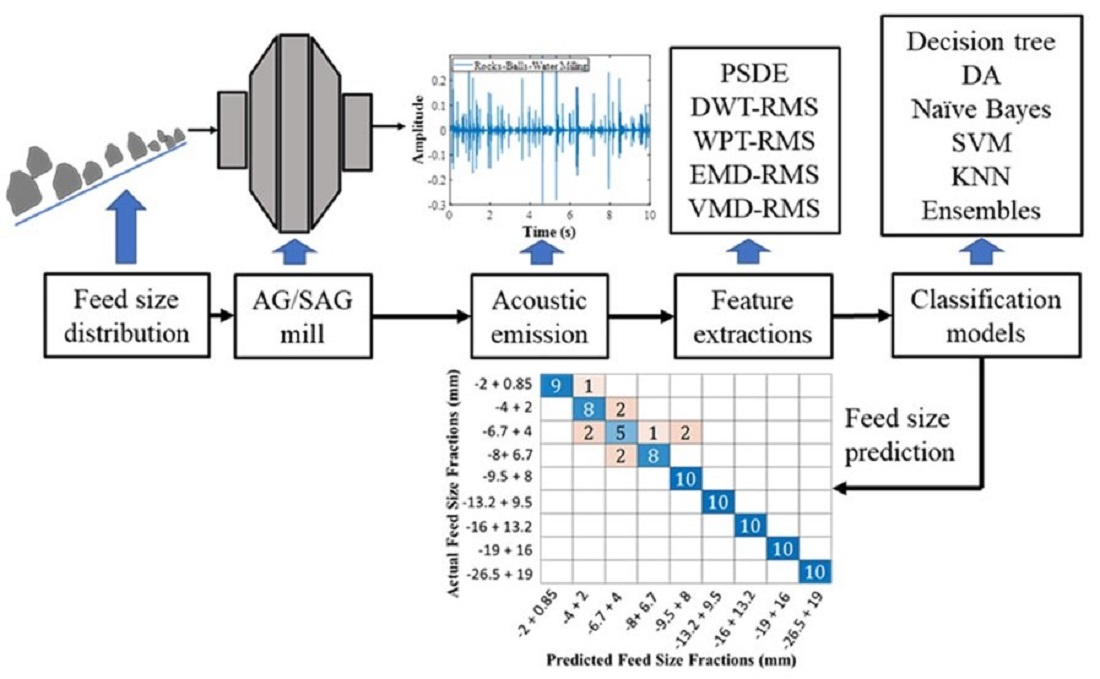
2. Experimental Method

2.1. Feed Size Variations, Grinding Studies, and Acoustic Measurements

The iron ore sample used in the study was classified into different fractions as shown in

Table 1. Feed particle size fractions and classification.

Class	Feed Size Fractions (mm)
1	−2 + 0.85
2	−4 + 2
3	−6.7 + 4
4	−8 + 6.7
5	−9.5 + 8
6	−13.2 + 9.5
7	−16 + 13.2
8	−19 + 16
9	−26.5 + 19

(photographs of the feed size fractions are provided in the Supplementary Document). Grinding was performed for the different mill feed size fractions using a laboratory-based AG/SAG mill (30 cm diameter to 15 cm length) connected to an acoustic sensor system [microphone and preamplifier (PreSonus—AudioBox iOne)] and a laptop computer. The microphone was positioned ~21 cm away from the toe section of the mill, as this is the region of the mill where significant acoustic emission intensities are produced [17]. Previous investigations published by the same authors provide a summary of the experimental setup [26]. A preliminary test was carried out with no load (empty mill) for one minute at different mill speeds of 40 rpm, 50 rpm, and 60 rpm, corresponding to 51.6, 64.5, and 77.4 critical speeds, respectively. In the actual study, the mill was operated with a charge made up of 2 kg of ore (~10 vol.%), steel balls (~8 vol.%), and 860 mL of water (~70 wt.% solids). The speed of the mill, unless otherwise specified, was constant at 58 rpm (~75% critical speed), and the grinding time was 5 min for each test. The acoustic sensor was used to record the mill acoustic signal during grinding (including the preliminary study) at a sampling frequency of 44.1 kHz [16]. The preliminary investigation was required to obtain acoustic sensed data (less varied signal) in order to select the appropriate statistical features from the acoustic signals. During grinding, the signal behaviour was visualised on the Audacity software platform, which was installed on the laptop computer. After each test, the acoustic signal is stored as a .wave file and exported to MATLAB platform for analysis. The grinding tests were performed in a controlled laboratory (quiet environment) to attenuate the interferences of any source of environmental noise. The mineralogical and chemical composition of the sample (XRF and XRD), as well as the mill and sensor specifications and experimental conditions, are reported in the supplementary document.

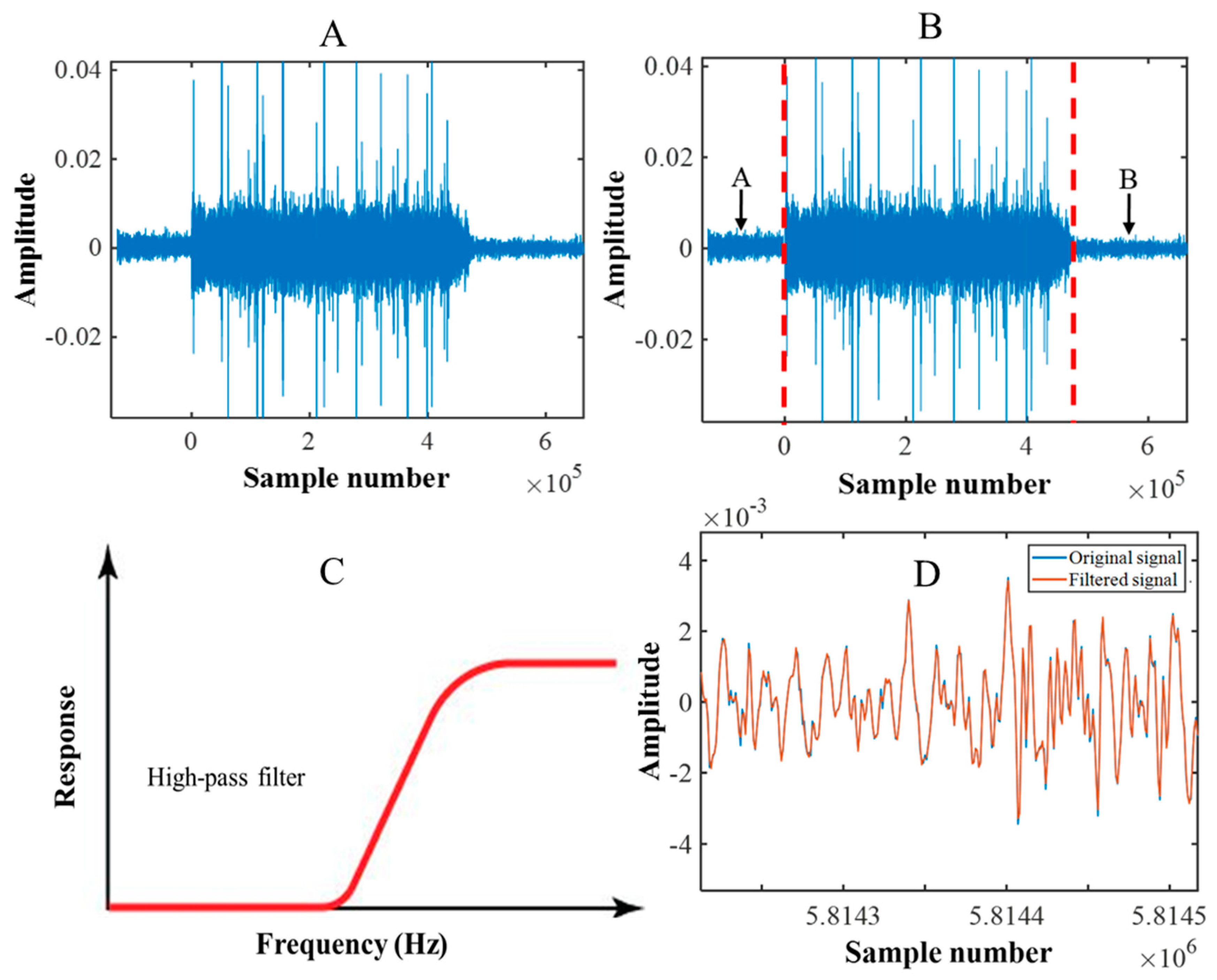
2.2. Acoustic Signal Data Collection and Pre-Processing

The acoustic emissions recorded from the mill fed with different size fractions of ore were analysed using the MATLAB R2020b software (Statistics and Machine Learning Toolbox—Classification Learner App). The first 30 s of acoustic data (1,323,000 sample points) were sampled from the entire 5 min of grinding time for the analysis, focusing on the acoustic response (sensitivity) of the different feed size fractions before disintegrating over time. The sampled sensed acoustic data provided enough information to represent each feed size fraction while reducing computational time. The signal was pre-processed by cropping out the pre-trigger and post-trigger signals, as well as by removing the background noise interference using the finite impulse response filter (FIR) [25]. Furthermore, the Savitzky–Golay filtering technique (also known as digital smoothing polynomial or least square smoothing filter) was applied to smoothen and improve signal quality [35]. This filtering technique was selected among other simple techniques, such as the moving average filter, because it has an extensive application and is preferred when the best polynomial order and frame length are estimated [35]. It tends to reduce or smooth out the noise of a signal while preserving the information of the original signal, such as shape, amplitude, peak height, width, and high-frequency components [35,36,37]. Figure 1 illustrates the step-by-step approach for processing the mill acoustic emission signals.

3. Preliminary Statistical Feature Extraction

To ascertain the most suitable statistical feature for the signal transforms, eight different statistical features, including root mean square (RMS), mean absolute value (MAV), the maximum (Max), standard deviation (SD), variance (Var), spectral skewness (SS), spectral kurtosis (SKur), and peak factor (PF) were considered as shown in

Table 2. Statistical feature selections.

Statistical Features	Equations	Number
Root mean square (RMS)	$RMS=\sqrt{\frac{1}{\Delta T}\underset{0}{\overset{\Delta t}{\int }}{AE}^2\left(t\right)dt}$	(1)
Mean absolute value (MAV)	$MAV=\frac{1}{N}{\displaystyle \sum _{i=1}^N}{|X_i-\mu |}^2$	(2)
Maximum (Max)	The maximum peak or value of a given acoustic signal	-
Standard deviation (SD)	$SD=\sqrt{\frac{1}{N}{\displaystyle \sum _{i=1}^N}{(X_i-\mu )}^2}$	(3)
Variance (Var)	$Var=\frac{1}{N}{\displaystyle \sum _{i=1}^N}{(X_i-\mu )}^2$	(4)
Skewness (SS)	$SS=\frac{1}{N}\frac{{\sum }_{i=1}^N{(X_i-\mu )}^3}{{SD}^3}$	(5)
Kurtosis (SKur)	$SKur=\frac{1}{N}\frac{{\sum }_{i=1}^N{(X_i-\mu )}^4}{{SD}^4}$	(6)
Peak factor (PF)	$PF=\frac{Max}{RMS}$	(7)

Where AE is the acoustic emission signal, N is the number of discretise AE data set within ΔT, ΔT is the integral time constant, t is the set time, i indicates the data values in the set under consideration, X is the data values, and μ is the mean value of the data set.

[38,39,40].

These features were first applied to the mill acoustic signal recorded from an empty mill revolution at 40 rpm, 50 rpm, and 60 rpm in the preliminary study. It was identified that the acoustic emission level intensity of an empty mill (no load), revolving at different speeds, has less variation in acoustic intensity characteristics (more stationary) [18]. The acoustic signal (10 s) corresponding to every speed was selected and sectioned into 10 frames containing 44,100 data points. Each feature was estimated for the different frames (10 times) and compared using the coefficient of variation (CoV). CoV is the relative variability of data expressed as the ratio of standard deviation to the arithmetic mean [41]. The acceptance criterion for estimating the performance of the features was set to 5% of the CoV.

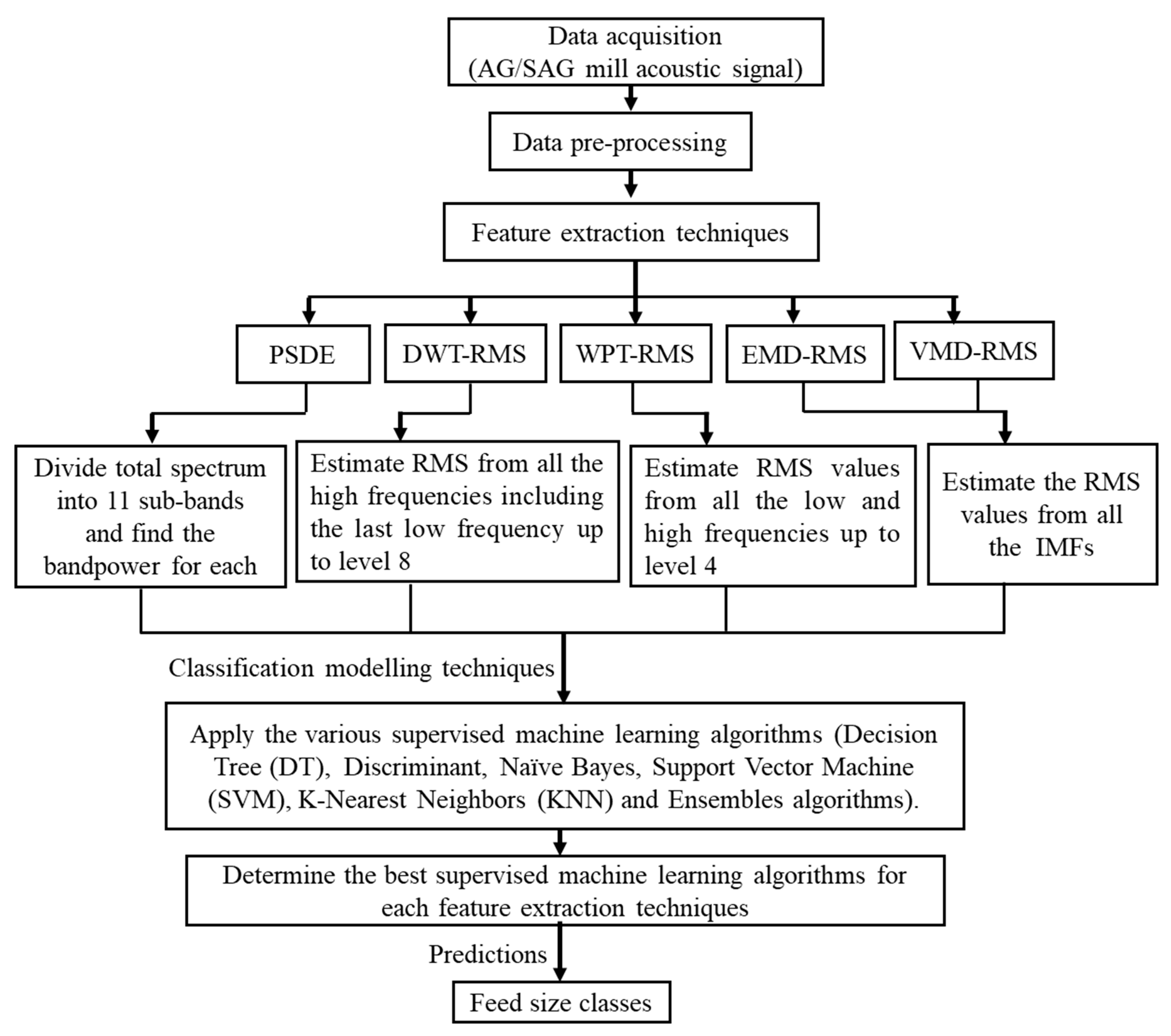
4. Feature Extraction Techniques for Mill Feed Size Acoustic Estimation

The recorded signals from the sensor during the grinding experiment were initially presented as time–amplitude domain acoustic signals. In this study, different transforms were applied to the time–amplitude domain acoustic signal to extract features as input feature vectors for modelling. The different transforms employed include power spectral density (PSDE), discrete wavelet transform (DWT), wavelet packet transform (WPT), empirical mode decomposition (EMD), and variational mode decomposition (VMD) [11]. In the PSDE analysis, the total spectrum was sub-divided into 11 bands, and the bandpowers were estimated as input features for the machine learning [14]. In addition, the root mean square values were also deduced from the DWT, WPT, EMD, and VMD as statistical input feature vectors for the modelling process.

4.1. Power Spectral Density Estimate (PSDE)

The time–amplitude domain signal is transformed into power spectral density estimate (PSDE) using the Welch’s method. PSDE is the power measurement variation within a signal, measured as a function of frequency [42]. Applying Welch’s method, the mill acoustic signal, denoted by x[n], is partitioned into a number of frames (segments) by multiplying a specified window function (Hanning), which is represented in Equations (8)–(11) [17,24,43,44,45].

Windowed mill signal:

$$X_m\left[n\right]=w\left[n\right]X\left[n+\left(m-1\right)R\right],n=0,1,2,\dots ,N-1,m=1,2,\dots ,M$$

(8)

where N is the window length, R is the window size, M is the frame number, and the N-point discrete Fourier transform (DFT) of the windowed mill signal, represented by X_m[k], is expressed as:

$$X_m\left[k\right]={\sum }_{n=0}^{N-1}{x}_m\left[n\right]e^{-j2\pi k/N};k=\mathrm{0,1},\dots ,N-1$$

(9)

Here, let S_m[k] be the PSDE of the windowed mill signals derived from the periodogram technique, as follows:

$$S_m\left[k\right]=\frac{1}{N}{\left|X_m\left[k\right]\right|}^2;k=\mathrm{0,1},\dots ,N-1$$

(10)

The Welch PSDE (improved averaged periodogram), given by S[k], is deduced by finding the average of the periodograms over frames as:

$$S\left[k\right]=\frac{1}{M}{\sum }_{m=0}^{M-1}{S}_m\left[k\right];k=\mathrm{0,1},\dots ,N-1$$

(11)

The criteria for computational parameters used in this work can be found in [25]. A quantitative approach was developed to quantify the total energy (bandpower) within a frequency spectrum. The frequency spectrum from 0–22 kHz was divided into 11 frequency bands of 2 kHz. The bandpower in each frequency band was computed and used as input features for the classification model.

4.2. Discrete Wavelet Transform (DWT)

Wavelet transform (WT) is used to extract information from a transient or non-stationary signal in both time and frequency [11,46]. WT can be classified into two types: the continuous wavelet transform (CWT), and the discrete wavelet transform (DWT). The CWT of a signal is defined as the integration of the product of the original signal x(t) and the son wavelet over a period, given in the expression as shown in Equation (12) [46,47,48]:

$$CWT\left(a,b\right)={\int }_{-\infty }^{+\infty }x\left(t\right){\psi }_{a,b}\left(t\right)dt=\frac{1}{\sqrt{a}}{\int }_{-\infty }^{+\infty }x\left(t\right)\psi (\frac{t-b}{a})dt$$

(12)

where a is the scalar factor, b is the translation factor, ψ_a.b(t) is the son wavelet, and ψ(t) is the mother wavelet.

For the DWT, the original signal is subjected to a low-pass filter and high-pass filter to obtain outputs of the low-frequency component (approximation coefficient) and high-frequency component (detail coefficient), respectively. The DWT of a given continuous signal x(t) is expressed in Equations (13) and (14) [46,49]:

$$DWT\left(a,b\right)={\int }_{-\infty }^{+\infty }x\left(t\right){\psi }_{a,b}\left(t\right)dt$$

(13)

$${\psi }_{\left(a,b\right)}(t)=\frac{1}{\sqrt{2^j}}\psi \left(\frac{t-2^{j}k}{2^j}\right)$$

(14)

where ψ_a,b defines the bases of wavelet functions, deduced from translated and dilated of the mother wavelet using the dilation a (2^j) and translation b (2^jk) parameters, respectively.

In this paper, DWT was considered for analysis using the fourth-order Daubechies (Db4) wavelet function [50]. The original acoustic signal was first decomposed into low-frequency components (approximation) and high-frequency components (detail). The low-frequency component sub-band was further decomposed into approximation and detail sub-bands. The procedure was repeated multiple times until the eighth stage for a fine-scale analysis. The detail components, including cD1, cD2, cD3, cD4, cD5, cD6, cD7, cD8, and the eight-decomposition level approximation component cA8, were selected. Following that, the RMS values were determined and used as input feature vectors to the machine-learning algorithms to estimate the feed particle size inside the AG/SAG mill.

4.3. Wavelet Packet Transform (WPT)

The framework of the wavelet packet transform (WPT) is similar to DWT and provides a better frequency resolution [48]. In DWT, the decompositions are iteratively focused on the low-frequency components (approximation coefficient), whereas in the WPT, the decomposition is simultaneously applied to both the low-frequency component (approximation coefficient) and high-frequency component (detail coefficient) sub-bands at every level [49]. During the decomposition process, any lost information in the low-frequency component is allocated to the high-frequency component. The Db4 wavelet function was used to decompose the acoustic signal until the fourth-level wavelet packet decomposition (four-layer structure). In all, 16 wavelet packet coefficients were obtained. The RMS values were ascertained for all the coefficients or sub-bands and used as input vectors in the machine-learning modelling.

4.4. Empirical Mode Decomposition (EMD)

EMD algorithm introduced by Huang et al. (1998) is used for analysing non-stationary and nonlinear time series signals [51,52]. The algorithm was employed initially to decompose a time-series signal into low-frequency components and high-frequency components (different resolutions). In the EMD, the low- and high-frequency parts are also referred to as residual and Intrinsic Mode Functions (IMF), respectively. The low-frequency component (residual) is considered a new signal and further decomposed into new low- and high-frequency components. The procedure is then repeated a given number of times, and the IMF parts were considered for analysis. Given a time series mill acoustic signal y(t), the following steps are taken using the EMD [11,52,53]:

• Determine all the local minima and maxima (extrema) of the given signal y(t).
• Estimate the lower envelope, e_min(t), and upper envelope, e_max(t), by interpolation of the extrema.
• The local average or mean, r(t) = [e_min(t) + e_max(t)]/2 of the envelope as the “low-pass” center, also known as the residual, is computed.
• Extract the first high-frequency component (IMF), as known as the detail component as d(t) = y(t) − r(t).
• Iterate the procedure on the residual r(t) until all the IMFs are acquired.

After the decomposition, the EMD algorithmic method presents the signal y(t) as the summation of all the IMFs and a final residual [53]:

$$y\left(t\right)={\sum }_{i=1}^n{h}_i\left(t\right)+r_n\left(t\right)$$

(15)

where h_i(t), i = 1…n are the IMFs and r_n(t) is the final residual.

The RMS of all the IMF components (9) were determined and used as input feature vectors in the machine-learning models.

4.5. Variational Mode Decomposition (VMD)

Similar to the EMD, VMD is a relatively novel and non-recursive decomposition algorithm, which is used for signal processing. While EMD is susceptible to noise, which can cause problems in mode mixing, the VMD algorithm has proven to overcome mode mixing and reduce the noise effect [54,55]. The algorithm is used to decompose non-stationary signals into multiple modes (IMFs or sub-signals), with limited frequency bandwidths and center frequency for solving variational problems [54,55]. It employs the variational model to search for and achieve optimal solutions. In all, the RMS of 10 IMF components were calculated and used as input feature vectors in the machine-learning models.

5. Machine Learning Classification Models’ Intuition

Machine learning is the process of training a machine to learn and make accurate predictions, or perform some given task when data are fed into it [29]. All machine-learning models can broadly be classified into supervised, semi-supervised, unsupervised, and reinforcement learning. Supervised learning involves developing predictive models from a series of functions that maps input and output data, whereas unsupervised learning employs machine-learning algorithms to groups and predicts unlabelled datasets based on only the input data [56]. Supervised learning can further be grouped into classification and regression models, whereas unsupervised learning is classified as clustering. In comparison, the results of supervised machine learning are more accurate and reliable than unsupervised machine learning [29]. Classification is one of the widely used machine-learning techniques in data mining, among other techniques [56]. Herein, six different standard classification techniques were applied, including Decision Tree (DT), discriminant analysis, Naïve Bayes (NB), Support Vector Machine (SVM), K-Nearest Neighbours (KNN), and ensembles [38,57].

5.1. Decision Tree

A decision tree (DT) is a type of algorithm that is commonly used in classification (binary and multi-class) and regression problems. It solves problems using tree representation, with each tree node corresponding to a class label and attributes represented on the internal nodes of the trees [29]. The decision tree algorithm becomes more accurate as the number of nodes increases. The technique builds a comprehensive and simplified algorithm for the classification process. The algorithm is not particularly powerful on its own, but when combined with other machine learnings and approaches, it transforms into a very powerful and useful machine learning for classification.

5.2. Discriminant Analysis

Discriminant analysis (DA), also known as linear discriminant analysis (LDA), is a technique used for classification and dimensionality reduction. As the name suggests, it employs a linear separator or decision boundary to distinguish some categories or classes. The LDA can be applied to both binary and multi-class classification problems. LDA is based on the assumption that different types of data can be separated linearly by projecting the data points onto a hyperplane (1D linear plane). In LDA, the data are projected from higher dimensions to lower dimensions unto a hyperplane in the feature space that is easily distinguishable [29]. Simply put, features in a large space are projected into a small subspace. The algorithm uses either inter-class separability (within-group variance) or between-class separability (between-group variance) to intelligently optimize the suitable linear plane (projection) to separate different categories of a given data. LDA is a very simple algorithm that leads to robust, reliable, and easy-to-understand classification results.

5.3. Naïve Bayes

Naïve Bayes (NB) is one of the simplest but most effective types of supervised classification algorithms that employs the Bayes theorem [29]. In the Naïve Bayes classification model, the algorithm assumes that the occurrence of one feature is independent of the other. The classifier develops models from a given set of data using a conditional probabilistic approach to learn certain features belonging to a class and make predictions [38]. The expression for the conditional probability is given in Equation (16) [58,59]:

$$P\left(A/B\right)=\frac{P\left(B/A\right)P\left(A\right)}{P\left(B\right)}$$

(16)

where A and B are the events, P(A/B) probability of occurrence of Event A, given that Event B is true, the P(B/A) probability of occurrence of Event B given that Event A is true, P(A) or P(B) is the probability of A or B.

The types of Naïve Bayes classifiers include the optimal, gaussian, multinomial, and Bernoulli.

5.4. Support Vector Machine

The Support Vector Machine (SVM) was developed in the 1960s and improved significantly in the 1990s when it began to gain popularity [60]. It is currently regarded as one of the most effective machine-learning algorithms, with high accuracy and less computational power. SVM is mostly used in classification objectives, though it can be applied to regression problems as well. The SVM distinctly classifies the dataset into classes or categories by searching for the optimum hyperplane or decision boundary (N-dimensional space, where N is the number of features) [29]. The number of features determines the dimension of the decision hyperplane. For example, the hyperplane becomes a line when the input features are two and increases with increasing the number of input features. The decision boundary is based on the maximum margin concept, which is implemented using support vectors. The main advantage of the SVM is its ability to handle a wide variety of classification problems, including high-dimensional and non-linearly separable problems [56].

5.5. K-Nearest Neighbours

The K-nearest neighbours (KNN) algorithm is one of the simplest and oldest machine-learning algorithms, developed to solve regression and classification problems. However, it has found broader application in classification problems. KNN entails selecting a number of K neighbours (e.g., 5) to determine the K neighbours of a new set of data based on the nearest distance measure, such as Euclidean, Cityblock, and Chebychev [38]. The Euclidean distance is usually used in most instances. The number of data points that constitute each category is determined, and the new data point is assigned to the category with the greatest number of neighbours. One significant advantage of KNN classification is its robustness and ability to handle large training datasets effectively [56].

5.6. Ensembles

The motivation of ensemble-based classification is to combine several different individual classifiers (often referred to as “weak learners”) into a single super-classifier with improved generalizability (a more robust and accurate model). In effect, the combined classifier provides better results than the individual classifiers incorporated in the combined classifier [61]. Ensembles can be built using either bagging or boosting approach. In the bagging approach, several different datasets are generated from the original dataset based on probability distribution (deterministic averaging process) from the original dataset. The generated datasets are trained independently in parallel with different classifiers (e.g., DT, LDA, KNN), and the outputs of the individual classifiers are combined to form the super-classifier (classification decision). The boosting approach, on the other hand, involves training the datasets generated from the original sequentially in an adaptive manner and combining them to form a super-classifier following a deterministic approach.

6. Methodology: Model Development Using Supervised Machine Learning Algorithms

In this study, six standard supervised classification models are employed to make predictions of nine different feed size ranges in laboratory AG/SAG mill grinding studies. This makes the problem multi-class classification. Using the MATLAB 2020b classification learner App, several labelled input data relating to feature extraction techniques (PSDE, DWT, WPT, EMD, and VMD) were initially fed into the classification algorithms. The classification learner App is a toolbox in MATLAB that enables users (experts or novices) to carry out general supervised machine-learning tasks (such as importing pre-processed data, extracting features, model selection and training, model tuning, etc.) by exploring different types of classification models without writing any code [62]. This method provided a simple overview (baseline knowledge) of how multiple classifiers will perform with the various feature extraction techniques under consideration, as well as a direction for future research. These reasons, as well as the data size (90 observations) obtained from the study, explain why this application was used. The applications provide a wide range of classifier options. However, in this study, a total of six classifiers, as discussed in Section 5, were applicable and taken into account. Following the training of the model, the optimal classifier can be assessed with a confusion matrix, receiver operating characteristic curve (ROC), area under the curve (AUC), and scatter plot.

The learner App allowed a quick analysis of the performance of the selected individual classification models (with confusion matrix) in the current study, followed by the selection of the two most appropriate classifiers. A total of 90 observations were used for the prediction of nine feed size classes. Since the data were carefully extracted, no data pre-processing stages were performed, and the data were devoid of missing values or outliers. Furthermore, the data were not subjected to standardization or normalization because they were essentially within a specific range with no extremities. The dataset was split into two; 72 observations were used as the training dataset (80%), and 18 observations for the testing dataset (20%) [38]. The task was to allow the machine to learn and understand data patterns from the trained dataset to make predictions of real-valued output (feed size classes) when tested on a new dataset. Since the total observations (90) were not sufficiently large, the k-fold cross-validation was used, with the k value set to 5 [38]. In each of the feature extraction datasets (PSDE, DWT-RMS, WPT-RMS, EMD-RMS, and VMD-RMS), the best two supervised classification algorithms were used. The objective was to identify which classification models can make the best prediction in each of the given data. Figure 2 presents the overview of the model development used in this study.

Classification Model Performance Evaluation Metrics

An evaluation metric converts a confusion matrix into values that can be used to compare the performance of various classification models or techniques [63]. The performance of the classification models was evaluated using four multifaceted metrics derived from the confusion matrix. These indicators include accuracy, precision/positive predicted value (PPV), sensitivity/recall, and F1 score [58,61]. The combination of the indicators provides a succinct evaluation of the model’s performance. The mathematical computations of the performance indicators are expressed in Equations (17)–(20) [38,64]:

$$Accuracy= \frac{(TP + TN)}{(TP + TN + FP + FN)}$$

(17)

$$Sensitivity or Recall = \frac{TP}{(TP + FN)}$$

(18)

$$Precision = \frac{TP}{(TP + FP)}$$

(19)

$$F1 score= \frac{2 \times (Precision \times Recall)}{(Precison + Recall)}$$

(20)

where TP is True Positive (model results classified as true, and the actual observation was true), TN is the True Negative (model results classified as false, and the actual observation was false), FP is False Positive (model results classified as true, but the actual observation was false), FN is False Negative (model results classified as false, but the actual observation was true).

7. Results and Discussion

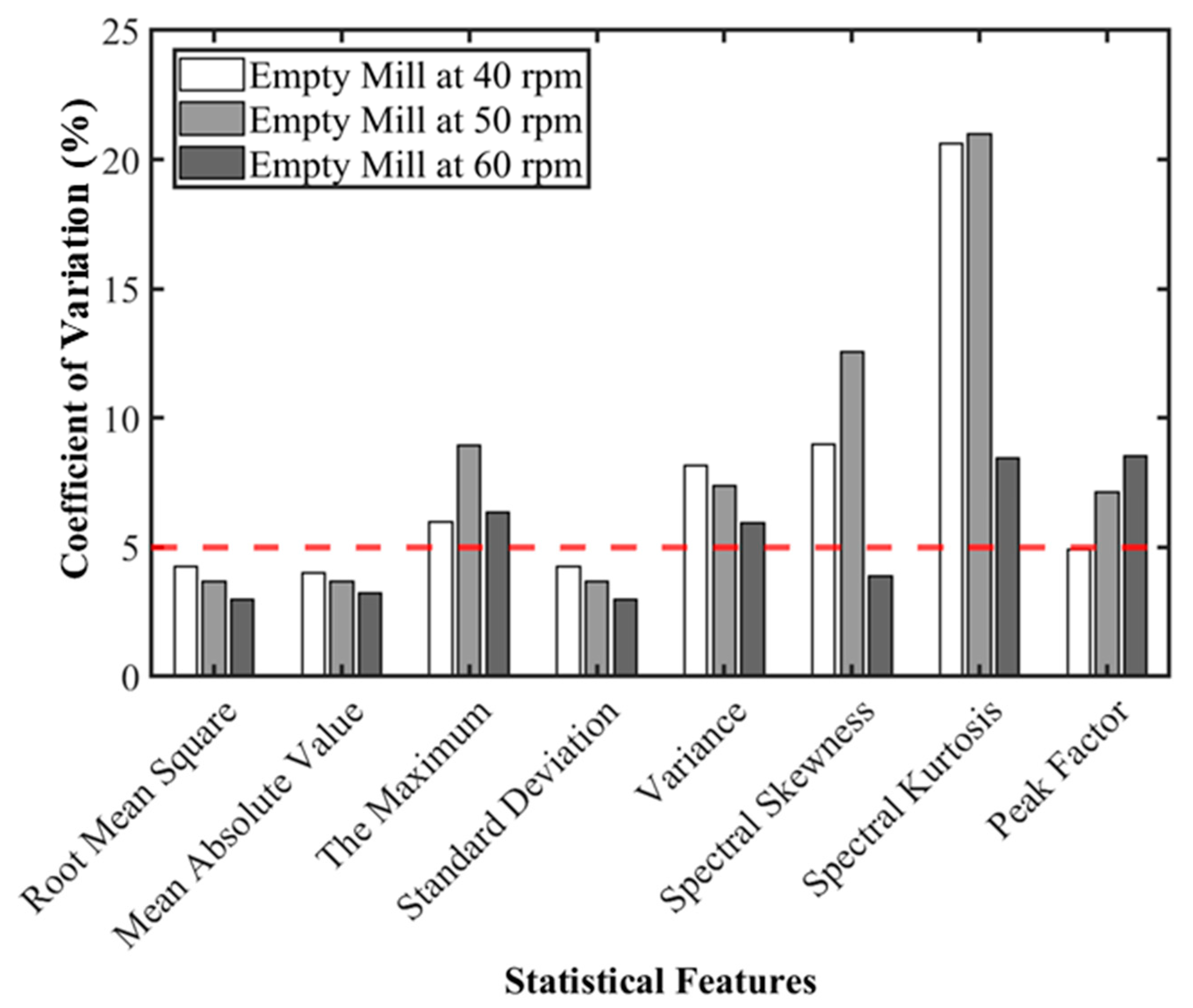
7.1. Statistical Feature Selection

Figure 3 shows the comparative statistical feature selection using the coefficient of variation (CoV). The selection criteria for the suitable statistical feature selection were set at 5% of the CoV. The feature below the 5% threshold (red short dashes horizontal line) of the CoV was considered as the relevant feature largely describing the acoustic signal, and vice versa. It was observed that the RMS, MAV, and SD of all the tested mill acoustic at 40 rpm, 50 rpm, and 60 rpm demonstrated an identical pattern below the set criterion. In this study, the RMS feature was chosen and combined with DWT, WPT, EMD, and VMD to generate the various input feature vectors for the model development. The RMS provides the average energy of the time domain signal [22].

7.2. Confusion Matrix for Feed Size Classification

The confusion matrix (also known as the error matrix) presents the summary of the performance assessment layout of classification problems (binary and multi-class classification) [58,63,64]. It is used to demonstrate how many classes (categories) were predicted correctly as true classes, and vice versa. The columns of the matrix are usually represented as the predicted classes, and the rows as actual or true classes. The correctly predicted classes are presented along the diagonal of the table, while the incorrect prediction is spread outside the diagonals [64]. As shown in Equations (17)–(20), several metrics can be deduced from a confusion matrix based on the true positive (TP), true negative (TN), false positive (FP), and false negative (FN) for performance evaluation analysis.

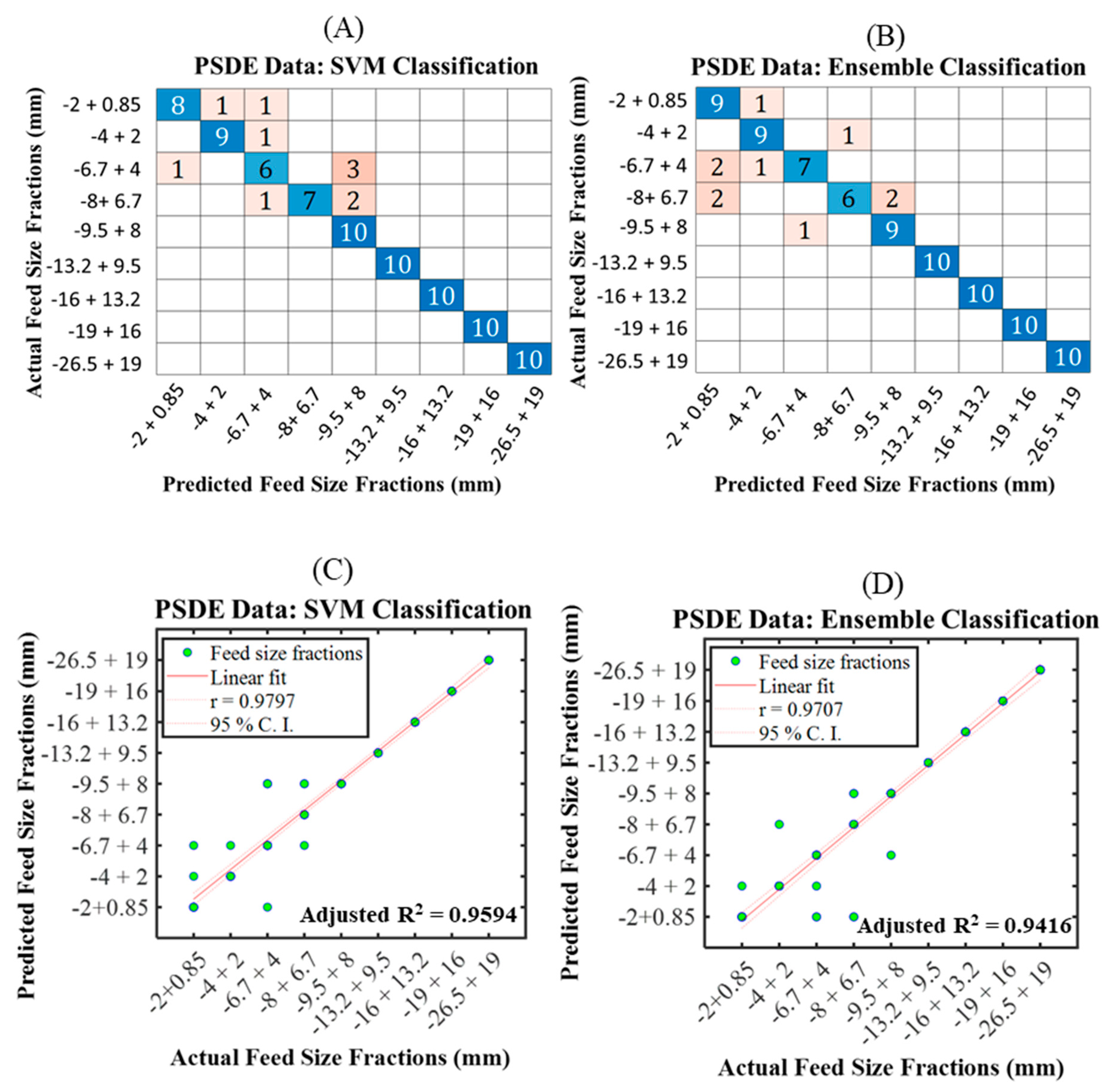
7.2.1. Model 1 with PSDE

A 9 × 9 confusion matrix based on PSDE data, as well as correlation plots for predicting different feed classes inside an AG/SAG, is shown in Figure 4. The results in Figure 4A,B show that, out of the six standard classification algorithms, the SVM (quadratic) and ensemble (subclass discriminant) classification algorithms provided closely related feed size predictions from the matrix diagonals with a suitable performance. The SVM classification perfectly predicted the coarse feed size classes from −9.5 + 8 mm to −26.5 + 19 mm and very good prediction of the relatively finer feed size classes of −2 + 0.85 mm and −4 + 2 mm with a low error. The model fairly predicted the feed size fractions of −6.7 + 4 mm and −8 + 6.7 mm. In the case of the ensemble classifier, similar prediction characteristics were obtained with 100% prediction associated with the coarse feed size classes from −13.2 + 9.5 mm to −26.5 + 19 mm.

From the parity plots in Figure 4C,D from the test data, the SVM and ensemble classifiers demonstrated strong correlations between the predicted and the actual feed size classes. This was evaluated with the coefficient of correlation (r), indicating ~0.98 and ~0.97 for SVM and ensemble classifiers, respectively. The SVM’s correlation was slightly greater than the ensemble approach, according to the r values. This was also reflected in their adjusted R² values.

It can be inferred from the confusion matrix and parity plots derived from SVM and ensemble classifiers that the acoustic emission produced by coarse feed size fractions is very distinct from that produced by somewhat finer feed fractions. As a result, the models can learn from the trained data and generate more accurate predictions with the tested data.

7.2.2. Model 2 with DWT–RMS

Figure 5 presents the confusion matrixes and correlation plots for classifying different feed size classes using DWT–RMS data. Using the input data from DWT–RMS, the linear discriminant and ensemble (subclass discriminant) classification algorithms were identified by the confusion matrixes diagonals to demonstrate an improved prediction of the feed size classes as shown in Figure 5A,B. Both classifiers showed flawless prediction at larger feed size ranges, from −9.5 + 8 mm to −26.5 + 19 mm, and they fluctuated when feed size fractions were reduced. To a large extent, the feed size classes below −9.5 + 8 mm showed an improved prediction and fewer mismatches with discriminant compared to the ensemble classifier. Specifically, the classification of feed size class −6.7 + 4 mm was not well predicted using the discriminant, whereas both feed classes of −6.7 + 4 mm and −8 + 6.7 mm were fairly classified by the ensemble algorithm. This is reflected well in the correlation plots in Figure 5C,D of the tested results, such that the discriminant classifier performed marginally better than the ensemble classifier with r values of ~0.99 and ~0.98, respectively, as well as their adjusted R² values.

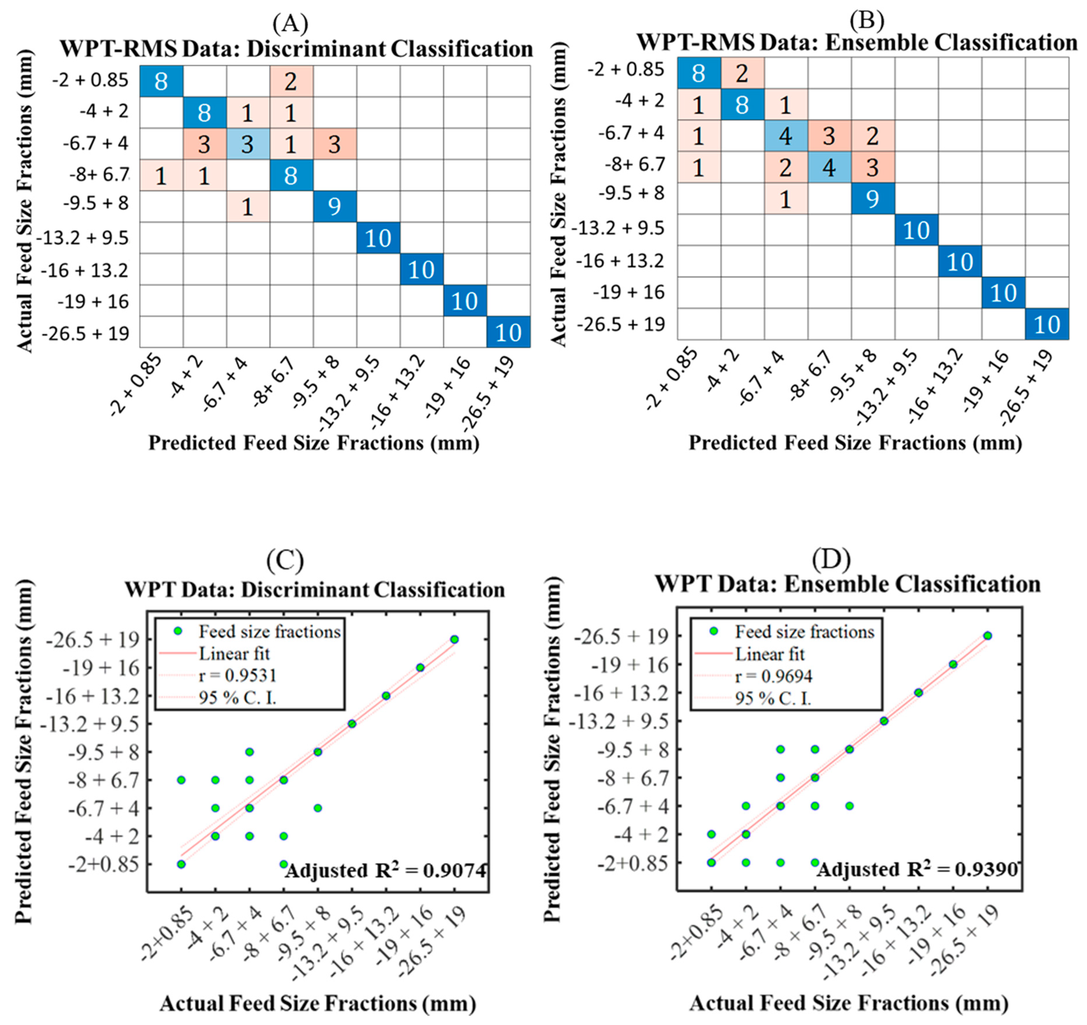
7.2.3. Model 3 with WPT–RMS

In the confusion matrixes and correlation plots shown in Figure 6, it was shown that the linear discriminant and ensemble (subclass discriminant) classification algorithms present better predictions after subjecting the WPT–RMS data to the six standard classification algorithms. In Figure 6A,B, it could be seen that both classifiers demonstrated close predictions of the feed size classes with excellent classification. The difference was much observed for relatively finer feed classes –6.7 + 4 mm and −8 + 6.7 mm. In comparison, the feed class of −6.7 + 4 mm was poorly predicted with less accuracy and very good prediction for −8 + 6.7 mm using the linear discriminant analysis, whereas both feed size classes demonstrated fair predictions with the ensemble classification.

According to the parity plot derived from the tested results in Figure 6C,D, the performance of the linear discriminant analysis was a little lower, with an r value of ~0.95, than the ensemble classifier, which had an r value of ~0.97. A similar trend was also observed in their adjusted R² values.

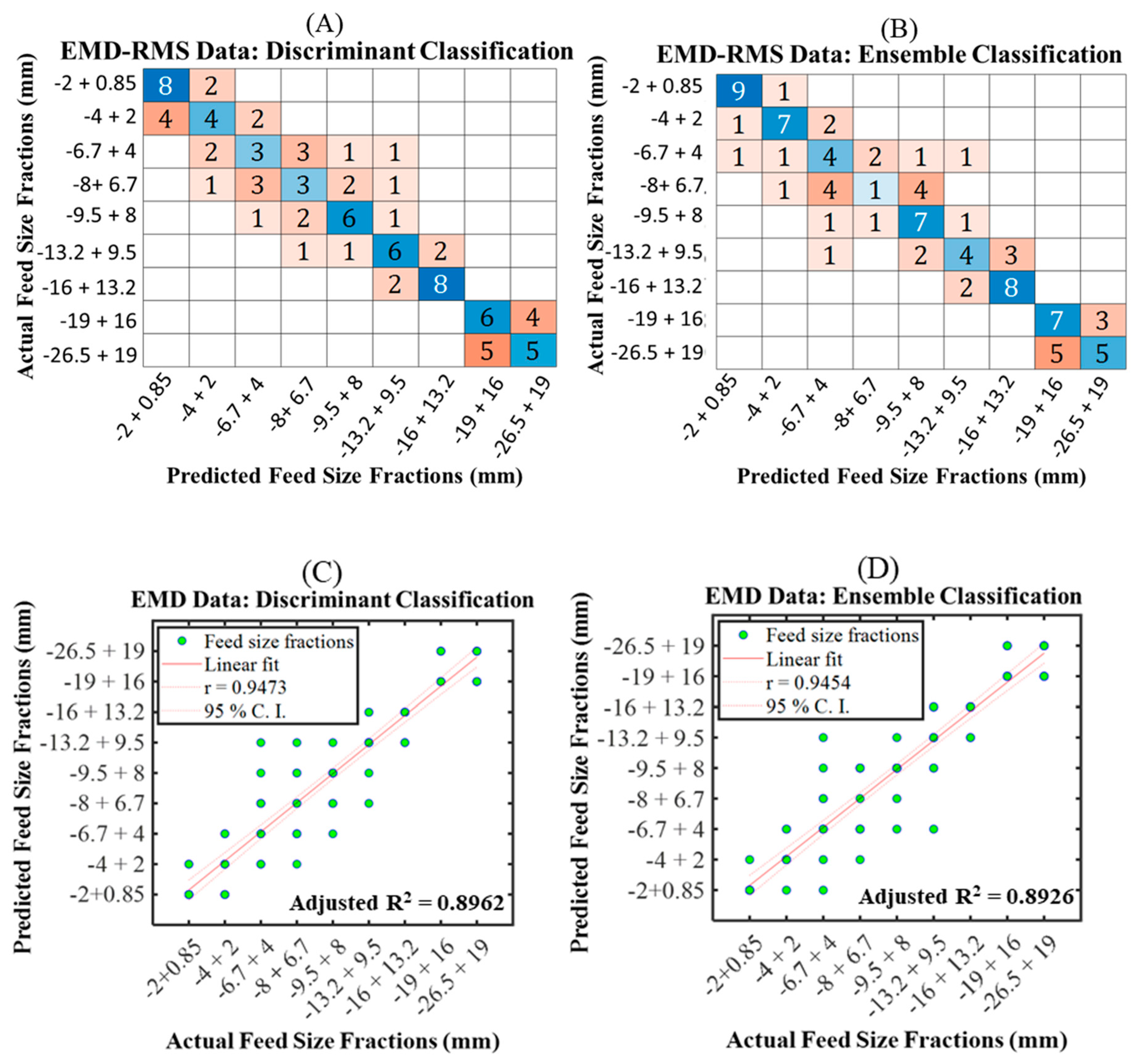
7.2.4. Model 4 with EMD–RMS

The confusion matrixes and correlation plots are provided in Figure 7, which shows the classification models that perform well with data generated from the EMD–RMS extraction technique. These models include the linear discriminant and ensemble (subclass discriminant) classifications (subclass discriminant). With the linear discriminant in Figure 7A, the most correctly predicted feed classes displayed along the matrix diagonal were identified as −2 + 0.85 mm (finer fraction) and −16 + 13.2 mm (coarser). It was also noted that the algorithm performed quite well with the coarser feed classes, starting from −9.5 + 8 mm to −26.5 + 19 mm. Relative to the finer feed size fractions, the performance of the discriminant classifier was quite poor. In Figure 7B, the ensemble classifier generally performed well in most of the feed classes predictions. The feed classes of −6.7 + 4 mm and −13.2 + 9.5 mm were not well-classified. The worst and poorly predicted feed class of the classifier was noted in −8 + 6.7 mm, which was able to predict one out of the total.

The strength of the linear discriminant and ensemble models in Figure 7C,D demonstrate that classifiers have a strong correlation between the actual and predicted feed size classes using the correlation coefficient (r) and adjusted R² values. From the correlation plots, the ensemble classifier was seen to marginally underperform the linear discriminant analysis.

7.2.5. Model 5 with VMD–RMS

The confusion matrixes of VMD–RMS data for identifying different feed size classes are shown in Figure 8A,B. Both linear discriminant and ensemble (subclass discriminant) classification methods displayed close and better performances for predicting different feed size classes in an AG/SAG mill using an acoustic response out of all the standard classification techniques examined. The coarser feed fractions from −9.5 + 8 mm to −26 + 19 mm were highly predicted and were identified to be the same for both classifiers. The differences in the prediction performance lie around the relatively finer feed fractions. The discriminant algorithm slightly underperformed for feed classes from −2 + 0.85 mm and −4 + 2 mm, and slightly outperformed feed classes of −6.7 + 4 mm and −8 + 6.7 mm when compared to the ensemble classifier. The prediction errors were noted to be widely diffused over the other feed classes.

The strength of the correlation plots produced from the tested results is shown in Figure 8C,D for both classifiers. In general, the classifiers have a good match between the actual and predicted feed size classes. Nevertheless, the ensemble classifier outperformed the linear discriminant classifier by a small margin.

Given a specific dataset extracted from different feature extraction techniques, the most suitable classification models were identified as SVM (quadratic), LDA, and ensemble (subclass discriminant) classifiers. To a greater extent, the layout of the confusion matrixes of the classed classifiers showed that the feed size fractions are best predicted predominantly at coarse feed size fractions ranging from −9.5 + 8 mm to −26.5 + 19 mm, followed by relatively finer feed size fractions −2 + 0.85 mm and −4 + 2 mm. The classification performance of the feed size fractions of −6.7 + 4 mm and −8 + 6.7 mm is frequently observed to be underpredicted.

Generally, the confusion matrixes for most of the feature extraction techniques appear to suggest that acoustic emission of coarse feed size fractions (−9.5 + 8 mm to −26.5 + 19 mm) are more distinctive from one another, and they are easily identified and predicted by the classification algorithms. When the feed size distribution reduces to −8 + 6.7 mm and −6.7 + 4 mm, the mill acoustic response seems to be unclear and reduced their predictions by most of the classifiers and improved at finer feed size fractions (−2 + 0.85 mm and −4 + 2 mm).

7.3. Model Evaluation

Table 3. Classification performance evaluation criteria.

Feature Extraction Techniques	Suitable Classification Models	Model Performance Indicators
		Accuracy	Precision	Sensitivity/Recall	F1 Score
PSDE	SVM (Quadratic)	88.89	90.25	88.89	89.56
	Ensemble (subspace discriminant)	88.89	89.56	88.89	89.23
DWT-RMS	LDA	88.89	88.95	88.89	88.92
	Ensemble (subspace discriminant)	85.56	85.46	85.56	85.51
WPT-RMS	LDA	84.44	84.14	84.44	84.29
	Ensemble (subspace discriminant)	81.11	80.46	81.11	80.79
EMD-RMS	LDA	54.44	53.60	54.44	54.02
	Ensemble (subspace discriminant)	57.78	55.97	57.78	56.86
VMD-RMS	LDA	83.33	84.21	83.33	83.77
	Ensemble (subspace discriminant)	83.33	83.74	83.33	83.54

shows multiple model evaluation indicators for all the classification models applied in the study using Equations (17)–(20). It should be noted that these indicators are presented as a percentage of 100. The multiple evaluation indicators are necessary to provide a comprehensive understanding of the models’ performance. In addition, with the closely related confusion matrixes of the two classification models performed on each extraction technique dataset, the multiple indicators will provide enough information to distinguish the performance of one model from the other. The indicators include accuracy, precision, sensitivity (recall), and F1 score.

Considering the SVM and ensemble classification models on the PSDE feature extraction technique from Table 3, the accuracy and sensitivity metrics recorded the same value of 88.9%, making it difficult to evaluate which of them has a better performance. The differences between the two classifiers are noted in the precision and F1 score. The SVM classifier has a somewhat higher precision and F1 score relative to the ensemble classifier. These two metrics are reflected very well with the r and adjusted R² values obtained from the parity plots in Figure 4C,D. As a result, with acoustic emission data transformed into PSDE, the SVM classifier appears to be better suited for predicting different feed size fractions in AG/SAG mills.

Again, from Table 3, it could be seen that the LDA and the ensemble (subclass discriminant) were the most prevailing or common classification models that were suitable for improved feed size class predictions using the feature extraction obtained from DWT–RMS, WPT–RMS, EMD–RMS, and VMD–RMS. Notably, all four assessment indicators deduced from the confusion matrixes in Figure 5A,B and Figure 6A,B demonstrated that the LDA provides a better classification of the feed size classes than the ensemble (subclass discriminant) classifier, which was consistent with the coefficient of correlation (r) and adjusted R² results in Figure 5C,D and Figure 6C,D. In addition, in the VMD–RMS, the accuracy and sensitivity metrics recorded the same value of 83.33% for both LDA and ensemble classifiers. The precision and F1 score values were higher for the LDA when compared to the ensemble technique. The ensemble classifier, on the other hand, outperformed the LDA using the EMD–RMS, with all higher metric values favouring the ensemble classifier. However, the level of predictions using the EMD–RMS technique demonstrated the least performance, even with the ensemble classifier. From the evaluation metrics, the degree of success was within the range of 50%. This appears to suggest that the input features derived from the EMD technique, combined with RMS, were not suitable for classifying multi-class feed size fractions in the AG/SAG mill.

Generally, from the confusion matrix evaluation metrics, as well as the correlation coefficient (r) and adjusted R², the study identified that feature vector representation from the PSDE method, coupled with the SVM (quadratic) classification algorithm, can provide the optimum classification of different feed size fractions during AG/SAG mill grinding operations. This was followed by the ensemble classifier applied to the same PSDE dataset. The LDA and ensemble (subclass discriminant) were found to be the most prevalent classification methods for improving feed size fraction predictions within an AG/SAG mill employing mill acoustic feature extractions, such as PSDE, DWT, WPT, EMD, and VMD.

8. Conclusions

The study investigated the performance of six standard classifications in predicting different feed size fractions inside an AG/SAG mill by extracting feature vectors from the mill acoustic response using five different extraction techniques. The classification models or algorithms include Decision Tree (DT), Linear Discriminant Analysis (LDA), Naïve Bayes (NB), Support Vector Machine (SVM), K-Nearest Neighbours (KNN), and ensembles techniques, while the feature extraction techniques, such as power spectral density estimate (PSDE), discrete wavelet transform (DWT), wavelet packet transform (WPT), empirical mode decomposition (EMD), and variational mode decomposition (VMD) coupled with statistical root mean square (RMS), were used. The performance of the models was estimated using confusion matrix-derived evaluation metrics, such as accuracy, precision, sensitivity (recall), and F1 score. The major findings in the study are outlined as follows:

(a)

The root mean square (RMS), mean absolute value (MAV), and standard deviation (SD) were identified as the most suitable statistical features for representing the mill acoustic signal with minimal variance.

(b)

The mill acoustic emission response is sensitive to different mill feed size fractions, such that an increase in the mill feed size ranges increases the acoustic emission.

(c)

All feature extraction techniques (PSDE, DWT, WPT, and VMD), except the EMD, were identified to give improved performance in classifying different feed size distributions inside AG/SAG mill.

(d)

The suitable extraction techniques and their respective classification algorithms for improved SAG mill feed size prediction are observed as follows: PSDE–SVM, DWT–LDA, WPT–LDA, EMD-ensemble, and VMD–LDA. The LDA and ensemble classifiers were noted to provide promising algorithms for improving feed size distribution in almost all the signal feature extraction techniques. The data extraction with PSDE combined with SVM classifier demonstrated the best degree of prediction for a sudden change in feed size fraction inside the SAG mill using the performance evaluation metrics such as accuracy, precision, sensitivity, and F1 score.

(e)

Mill acoustic emission and supervised machine-learning classification models can be used to provide more insight into the changing feed size distribution of SAG mills. The study’s findings could be beneficial to the comminution circuit by serving as a proxy measure for predicting the sudden feed size fluctuations in real time and assessing the efficiency of upstream processes like crushing and screening. This can result in faster decision-making and more timely intervention by mill operators. Though the current work is constrained to (i) A batch sample rather than continuous feed (blending); and (ii) A small-scale mill rather than an industrial mill, the study provides directions for future applications in large-scale AG/SAG mills.

References

1. Morrell, S. The influence of feed size on autogenous and semi-autogenous grinding and the role of blasting in its manipulation. In Proceedings of the XXII International Mineral Processing Congress, Cape Town, South Africa, 29 September–3 October 2003. [Google Scholar]
2. Hahne, R.; Pålsson, B.I.; Samskog, P.O. Ore characterisation for—And simulation of—Primary autogenous grinding. Miner. Eng. 2003, 16, 13–19. [Google Scholar] [CrossRef]
3. Morrell, S.; Valery, W. Influence of feed size on AG/SAG mill performance. In Proceedings of the SAG2001, Vancouver, BC, Canada, 30 September–3 October 2001; pp. 203–214. [Google Scholar]
4. Núñez, F.; Silva, D.; Cipriano, A. Characterization and Modeling of Semi-Autogenous Mill Performance Under Ore Size Distribution Disturbances. IFAC Proc. Vol. 2011, 44, 9941–9946. [Google Scholar] [CrossRef]
5. Asamoah, R.K.; Baawuah, E.; Greet, C.; Skinner, W. Characterisation of Metal Debris in Grinding and Flotation Circuits. Miner. Eng. 2021, 171, 107074. [Google Scholar] [CrossRef]
6. Joseph-Soly, S.; Asamoah, R.K.; Skinner, W.; Addai-Mensah, J. Superabsorbent dewatering of refractory gold concentrate slurries. Adv. Powder Technol. 2020, 31, 3168–3176. [Google Scholar] [CrossRef]
7. Forson, P.; Zanin, M.; Abaka-Wood, G.; Skinner, W.; Asamoah, R.K. Flotation of auriferous arsenopyrite from pyrite using thionocarbamate. Miner. Eng. 2022, 181, 107524. [Google Scholar] [CrossRef]
8. Asamoah, R.K.; Skinner, W.; Addai-Mensah, J. Pulp mineralogy and chemistry, leaching and rheological behaviour relationships of refractory gold ore dispersions. Chem. Eng. Res. Des. 2019, 146, 87–103. [Google Scholar] [CrossRef]
9. Asamoah, R.K.; Zanin, M.; Skinner, W.; Addai-Mensah, J. Refractory gold ores and concentrates part 2: Gold mineralisation and deportment in flotation concentrates and bio-oxidised products. Miner. Process. Extr. Metall. 2019, 130, 269–282. [Google Scholar] [CrossRef]
10. Forson, P.; Zanin, M.; Skinner, W.; Asamoah, R. Differential flotation of pyrite and arsenopyrite: Effect of hydrogen peroxide and collector type. Miner. Eng. 2021, 163, 106808. [Google Scholar] [CrossRef]
11. Nayak, D.K.; Das, D.P.; Behera, S.K.; Das, S.P. Monitoring the fill level of a ball mill using vibration sensing and artificial neural network. Neural Comput. Appl. 2020, 32, 1501–1511. [Google Scholar] [CrossRef]
12. Behera, B.; Mishra, B.; Murty, C. Experimental analysis of charge dynamics in tumbling mills by vibration signature technique. Miner. Eng. 2007, 20, 84–91. [Google Scholar] [CrossRef]
13. Thornton, A.; Pethybridge, T.; Dunn, R.; Rivett, T. SAG Mill Control at Northparkes Mines (Not So Hard after All); MIPAC Report; MIPAC: Albion, QLD, Australia, 2005. [Google Scholar]
14. Spencer, S.; Sharp, V.; Campbell, J.J.; Holmes, R.J.; Rowlands, T.; Barker, D.G.; Davey, K.J.; Phillips, P.L. Prediction of AG/SAG mill variables from surface vibrations. In Proceedings of the XXIII International Mineral Processing Congress, Turkish Mining Development Foundation, Istanbul, Turkey, 3–8 September 2006. [Google Scholar]
15. Wei, D.; Craig, I.K. Grinding mill circuits—A survey of control and economic concerns. Int. J. Miner. Process. 2009, 90, 56–66. [Google Scholar] [CrossRef]
16. Owusu, K.B.; Karageorgos, J.; Greet, C.; Zanin, M.; Skinner, W.; Asamoah, R.K. Predicting mill feed grind characteristics through acoustic measurements. Miner. Eng. 2021, 171, 107099. [Google Scholar] [CrossRef]
17. Aldrich, C.; Theron, D.A. Acoustic estimation of the particle size distributions of sulphide ores in a laboratory ball mill. J. S. Afr. Inst. Min. Metall. 2000, 100, 243–248. [Google Scholar]
18. Zeng, Y.; Forssberg, E. Effects of operating parameters on vibration signal under laboratory scale ball grinding conditions. Int. J. Miner. Process. 1992, 35, 273–290. [Google Scholar] [CrossRef]
19. Zeng, Y.; Forssberg, E. Application of digital signal processing and multivariate data analysis to vibration signals from ball-mill grinding. Trans. Inst. Min. Sect. C-Miner. Process. Extr. Metall. 1993, 102, 39–43. [Google Scholar]
20. Zeng, Y.; Forssberg, E. Application of vibration signals to monitoring crushing parameters. Powder Technol. 1993, 76, 247–252. [Google Scholar] [CrossRef]
21. Zeng, Y.; Forssberg, E. Monitoring grinding parameters by signal measurements for an industrial ball mill. Int. J. Miner. Process. 1993, 40, 1–16. [Google Scholar] [CrossRef]
22. Zeng, Y. Vibration Signal Analysis in Comminution. Ph.D. Thesis, Luleå Tekniska Universitet, Luleå, Sweden, 1994. [Google Scholar]
23. Zeng, Y.; Forssberg, K. Vibration signal emission from mono-size particle breakage. Int. J. Miner. Process. 1996, 44–45, 59–69. [Google Scholar] [CrossRef]
24. Das, S.P.; Das, D.P.; Behera, S.K.; Mishra, B.K. Interpretation of mill vibration signal via wireless sensing. Miner. Eng. 2011, 24, 245–251. [Google Scholar] [CrossRef]
25. Owusu, K.B.; Zanin, M.; Skinner, W.; Asamoah, R.K. AG/SAG mill acoustic emissions characterisation under different operating conditions. Miner. Eng. 2021, 171, 107098. [Google Scholar] [CrossRef]
26. Owusu, K.B.; Skinner, W.; Asamoah, R. Feed hardness and acoustic emissions of autogenous/semi-autogenous (AG/SAG) mills. Miner. Eng. 2022, 187, 107781. [Google Scholar] [CrossRef]
27. Owusu, K.B.; Skinner, W.; Asamoah, R. Acoustic Sensor Frequencies and Mill Feed Properties—A Brief Review; Engineers Australia: Barton, ACT, Australia, 2021. [Google Scholar]
28. Owusu, K.B.; Greet, C.J.; Skinner, W.; Asamoah, R.K. Influence of lifter height on mill acoustics and performance. In Proceedings of the 5th International Future Mining Conference 2021, Online, 6–10 December 2021. [Google Scholar]
29. Dhall, D.; Kaur, R.; Juneja, M. Machine Learning: A Review of the Algorithms and Its Applications. In Proceedings of ICRIC 2019; Springer: Cham, Switzerland, 2020; pp. 47–63. [Google Scholar] [CrossRef]
30. Meylan, B.; Shevchik, S.A.; Parvaz, D.; Mosaddeghi, A.; Simov, V.; Wasmer, K. Acoustic emission and machine learning for in situ monitoring of a gold–copper ore weakening by electric pulse. J. Clean. Prod. 2021, 280, 124348. [Google Scholar] [CrossRef]
31. Al-Zubaidi, S.; Ghani, J.A.; Haron, C.H.C. Application of ANN in Milling Process: A Review. Model. Simul. Eng. 2011, 2011, 696275. [Google Scholar] [CrossRef]
32. Amankwaa-Kyeremeh, B.; Zhang, J.; Zanin, M.; Skinner, W.; Asamoah, R.K. Feature selection and Gaussian process prediction of rougher copper recovery. Miner. Eng. 2021, 170, 107041. [Google Scholar] [CrossRef]
33. Li, Y.; Bao, J.; Yu, A.; Yang, R. ANN prediction of particle flow characteristics in a drum based on synthetic acoustic signals from DEM simulations. Chem. Eng. Sci. 2021, 246, 117012. [Google Scholar] [CrossRef]
34. Zeng, Y.; Forssberg, E. Monitoring grinding parameters by vibration signal measurement—A primary application. Miner. Eng. 1994, 7, 495–501. [Google Scholar] [CrossRef]
35. Acharya, D.; Rani, A.; Agarwal, S.; Singh, V. Application of adaptive Savitzky–Golay filter for EEG signal processing. Perspect. Sci. 2016, 8, 677–679. [Google Scholar] [CrossRef] [Green Version]
36. Guiñón, J.L.; Ortega, E.; García-Antón, J.; Pérez-Herranz, V. Moving average and Savitzki-Golay smoothing filters using Mathcad. In Proceedings of the International Conference on Engineering Education, ICEE 2007, Coimbra, Portugal, 3–7 September 2007; pp. 1–4. [Google Scholar]
37. Liu, Y.; Dang, B.; Li, Y.; Lin, H.; Ma, H. Applications of Savitzky-Golay Filter for Seismic Random Noise Reduction. Acta Geophys. 2016, 64, 101–124. [Google Scholar] [CrossRef] [Green Version]
38. Mathew, S.K.; Zhang, Y. Acoustic-Based Engine Fault Diagnosis Using WPT, PCA and Bayesian Optimization. Appl. Sci. 2020, 10, 6890. [Google Scholar] [CrossRef]
39. Owusu, K.B.; Karageorgos, J.; Greet, C.; Zanin, M.; Skinner, W.; Asamoah, R.K. Acoustic Monitoring of Mill Pulp Densities. In Proceedings of the 6th UMaT Biennial International Mining and Mineral Conference, Tarkwa, Ghana, 4–7 August 2020. [Google Scholar]
40. Rangel-Magdaleno, J.; Peregrina-Barreto, H.; Ramirez-Cortes, J.; Morales-Caporal, R.; Cruz-Vega, I. Vibration Analysis of Partially Damaged Rotor Bar in Induction Motor under Different Load Condition Using DWT. Shock Vib. 2016, 2016, 3530464. [Google Scholar] [CrossRef]
41. Ospina, R.; Marmolejo-Ramos, F. Performance of Some Estimators of Relative Variability. Front. Appl. Math. Stat. 2019, 5, 43. [Google Scholar] [CrossRef]
42. Same, M.H.; Gandubert, G.; Gleeton, G.; Ivanov, P.; Landry, R., Jr. Simplified Welch Algorithm for Spectrum Monitoring. Appl. Sci. 2021, 11, 86. [Google Scholar] [CrossRef]
43. Kılıç, R.; Kumbasar, N.; Oral, E.A.; Ozbek, I.Y. Drone classification using RF signal based spectral features. Eng. Sci. Technol. Int. J. 2021, 28, 101028. [Google Scholar] [CrossRef]
44. Solomon, O., Jr. PSD Computations Using Welch’s Method; Power Spectral Density (PSD); Sandia National Lab.: Albuquerque, NM, USA, 1991; p. 23584. [Google Scholar]
45. Welch, P.D. The use of fast Fourier transform for the estimation of power spectra: A method based on time averaging over short, modified periodograms. IEEE Trans. Audio Electroacoust. 1967, 15, 70–73. [Google Scholar] [CrossRef] [Green Version]
46. Oliveira, M.O.; Reversat, J.H.; Reynoso, L.A. Wavelet Transform Analysis to Applications in Electric Power Systems. In Wavelet Transform and Complexity; InTech Open: London, UK, 2019; pp. 1–17. [Google Scholar] [CrossRef] [Green Version]
47. Plaza, E.G.; López, P.N. Analysis of cutting force signals by wavelet packet transform for surface roughness monitoring in CNC turning. Mech. Syst. Signal Process. 2018, 98, 634–651. [Google Scholar] [CrossRef]
48. Yen, G.; Lin, K.-C. Wavelet packet feature extraction for vibration monitoring. IEEE Trans. Ind. Electron. 2000, 47, 650–667. [Google Scholar] [CrossRef] [Green Version]
49. Zhang, Z.; Wang, Y.; Wang, K. Fault diagnosis and prognosis using wavelet packet decomposition, Fourier transform and artificial neural network. J. Intell. Manuf. 2013, 24, 1213–1227. [Google Scholar] [CrossRef]
50. Huang, F.; Wu, P.; Ziggah, Y. GPS Monitoring Landslide Deformation Signal Processing using Time-series Model. Int. J. Signal Process. Image Process. Pattern Recognit. 2016, 9, 321–332. [Google Scholar] [CrossRef]
51. Huang, N.E.; Shen, Z.; Long, S.R.; Wu, M.C.; Shih, H.H.; Zheng, Q.; Yen, N.-C.; Tung, C.C.; Liu, H.H. The empirical mode decomposition and the Hilbert spectrum for nonlinear and non-stationary time series analysis. Proc. Math. Phys. Eng. Sci. 1998, 454, 903–995. [Google Scholar] [CrossRef]
52. Dragomiretskiy, K.; Zosso, D. Variational mode decomposition. IEEE Trans. Signal Process. 2013, 62, 531–544. [Google Scholar] [CrossRef]
53. Labate, D.; La Foresta, F.; Occhiuto, G.; Morabito, F.C.; Lay-Ekuakille, A.; Vergallo, P. Empirical mode decomposition vs. wavelet decomposition for the extraction of respiratory signal from single-channel ECG: A comparison. IEEE Sens. J. 2013, 13, 2666–2674. [Google Scholar] [CrossRef]
54. Huang, Q.; Liu, X.; Li, Q.; Zhou, Y.; Yang, T.; Ran, M. A parameter-optimized variational mode decomposition method using salp swarm algorithm and its application to acoustic-based detection for internal defects of arc magnets. AIP Adv. 2021, 11, 065216. [Google Scholar] [CrossRef]
55. Vanitha, V.; Sophia, J.G.; Resmi, R.; Raphel, D. Artificial intelligence-based wind forecasting using variational mode decomposition. Comput. Intel. 2020, 37, 1034–1046. [Google Scholar]
56. Soofi, A.A.; Awan, A. Classification Techniques in Machine Learning: Applications and Issues. J. Basic Appl. Sci. 2017, 13, 459–465. [Google Scholar] [CrossRef]
57. Tewari, K.; Vandita, S.; Jain, S. Predictive Analysis of Absenteeism in MNCS Using Machine Learning Algorithm. In Proceedings of ICRIC 2019; Springer: Cham, Switzerland, 2020; pp. 3–14. [Google Scholar] [CrossRef]
58. Singh, P.; Chahal, D.; Kharb, L. Predictive Strength of Selected Classification Algorithms for Diagnosis of Liver Disease. In Proceedings of ICRIC 2019; Springer: Cham, Switzerland, 2020; pp. 239–255. [Google Scholar] [CrossRef]
59. Paul, Y.; Kumar, N. A Comparative Study of Famous Classification Techniques and Data Mining Tools. In Proceedings of ICRIC 2019; Springer: Cham, Switzerland, 2020; pp. 627–644. [Google Scholar] [CrossRef]
60. Zhu, G.; Blumberg, D.G. Classification using ASTER data and SVM algorithms;: The case study of Beer Sheva, Israel. Remote Sens. Environ. 2002, 80, 233–240. [Google Scholar] [CrossRef]
61. Sahu, S.K.; Mohapatra, D.P. A Review on Scalable Learning Approaches on Intrusion Detection Dataset. In Proceedings of ICRIC 2019; Springer: Cham, Switzerland, 2020; pp. 699–714. [Google Scholar]
62. Han, S.; Li, M.; Ren, Q. Discriminating among tectonic settings of spinel based on multiple machine learning algorithms. Big Earth Data 2019, 3, 67–82. [Google Scholar] [CrossRef] [Green Version]
63. Fatourechi, M.; Ward, R.K.; Mason, S.G.; Huggins, J.; Schlögl, A.; Birch, G.E. Comparison of Evaluation Metrics in Classification Applications with Imbalanced Datasets. In Proceedings of the 2008 Seventh International Conference On Machine Learning and Applications, San Diego, CA, USA, 11–13 December 2008. [Google Scholar] [CrossRef]
64. Patro, V.M.; Patra, M.R. Augmenting Weighted Average with Confusion Matrix to Enhance Classification Accuracy. Trans. Mach. Learn. Artif. Intell. 2014, 2, 77–91. [Google Scholar] [CrossRef] [Green Version]
65. Deniz, V. A study on the effect of ball diameter on breakage properties of clinker and limestone. Indian J. Chem. Technol. 2021, 19, 180–184. [Google Scholar]
66. Nava, J.V.; Llorens, T.; Menéndez-Aguado, J.M. Kinetics of Dry-Batch Grinding in a Laboratory-Scale Ball Mill of Sn–Ta–Nb Minerals from the Penouta Mine (Spain). Metals 2020, 10, 1687. [Google Scholar] [CrossRef]
67. Starkey, J.H.; Hindstrom, S.; Orser, T. Choosing a SAG mill to achieve design performance. In Proceedings of the CMP Conference, Ottawa, ON, Canada, 17–19 January 2023. [Google Scholar]
Figure 1. A step-by-step procedure for the signal pre-processing (A) raw acoustic emission (B) removal of pre-and-post signals, where A and B are the pre-signal and post-signal, respectively. The red short dashes vertical lines represent the pre-and-post cut-off parts of the signal (C) FIR filter development and (D) Savitzky–Golay filtering technique.
Powders 02 00018 g001
Figure 2. Flowsheet for model development.
Powders 02 00018 g002
Figure 3. Statistical feature selection for mill acoustic analysis using the coefficient of variation. The red short dashes horizontal line represents the threshold for the statistical feature selection criterion.
Powders 02 00018 g003
Figure 4. A plot showing (A) confusion matrix from SVM classification (B) confusion matrix from ensemble classification (C) correlation plot of SVM classification and (D) correlation plot of ensemble classification.
Powders 02 00018 g004
Figure 5. A plot showing (A) confusion matrix from discriminant classification (B) confusion matrix from ensemble classification (C) correlation plot of discriminant classification and (D) correlation plot of ensemble classification.
Powders 02 00018 g005
Figure 6. A plot showing (A) confusion matrix from discriminant classification (B) confusion matrix from ensemble classification (C) correlation plot of discriminant classification, and (D) correlation plot of ensemble classification.
Powders 02 00018 g006
Figure 7. A plot showing (A) confusion matrix from discriminant classification (B) confusion matrix from ensemble classification (C) correlation plot of discriminant classification, and (D) correlation plot of ensemble classification.
Powders 02 00018 g007
Figure 8. A plot showing (A) confusion matrix from discriminant classification (B) confusion matrix from ensemble classification (C) correlation plot of discriminant classification and (D) correlation plot of ensemble classification.
Powders 02 00018 g008