Heuristic and Bayesian Tornado Prediction in Complex Terrain of Southern Wyoming

Abstract

A heuristic technique for tornado forecasting in the complex terrain of southern Wyoming is proposed for the weather sciences community. This novel approach is based on seasonal tornado climatology and observed mesoscale conditions obtained from in-situ surface and Doppler weather radar sources. The methodology is applied to four severe thunderstorm events which formed tornadoes during the spring and summer months of 2018 and 2019 in Albany County of Wyoming. Tornadic evolution is associated with supercell thunderstorms forming along moisture convergence axes of a dryline and updraft interactions with air mass stretching and shearing over the complex terrain. Applying Bayes’ theorem to each case, there is a low to high (30 to 80%) posterior probability associated with vortex detection.

1. Introduction

Tornadoes are mesoscale weather systems, occasionally produced by severe thunderstorms, and pose a danger to life and property [1]. Although tornadoes are climatologically infrequent events in certain regions of the western United States [1,2,3], such phenomena have occurred in recent years over the complex terrain of Wyoming [4,5,6]. The challenges of predicting these weather systems involve different approaches.

Traditional tornado forecasting involves meteorologists interrogating local storm environments in real-time with three-dimensional radar sweeps of convection and subsequent subjective or automated tornado algorithm identification [6]. Another methodology rooted in climatology uses longer-term antecedent synoptic weather patterns over large geographical regions to form a prediction [3]. In the past two decades, high-resolution Eulerian numerical models simulate environmental conditions, kinematic flows, and internal storm dynamics of tornadic thunderstorms. However, these simulations struggle with spatial and temporal details, especially in mountainous regions like Wyoming [7]. In recent years, Convective Allowing Models (CAMs) have shown promise in predicting tornadoes at fine (50-m) grid scales [8]. Problematically, computing resources for such fine-scale tornadic predictions may become protracted and too expensive or simply unavailable. Finally, automated machine learning techniques based on rapid spatial recognition of storm patterns have demonstrated some success [9].

In retrospect, humans are very adept at solving forecasting problems in unique ways with shortcuts and assumptions [10]. These novel solutions are generally faster but may not be as accurate as their counterparts above. Consequently, a heuristic tornado forecasting methodology is presented based on the probabilities of seasonal event climatology and mesoscale meteorological predictors obtained from a dense real-time in-situ surface mesonetwork and dual-Doppler weather radar observations.

2. Research Motivation and Goal

The motivation for this study is based on a need to help weather forecasters predict high-altitude tornadoes with a heuristic paradigm [10] based on meteorological rules-of-thumb and practical assumptions. This work is performed to complement existing forecasting techniques. The goal of the study is to provide a simple yet powerful framework using Bayes’ theorem for tornado forecasting in the complex terrain of southern Wyoming.

Hypothesis Test

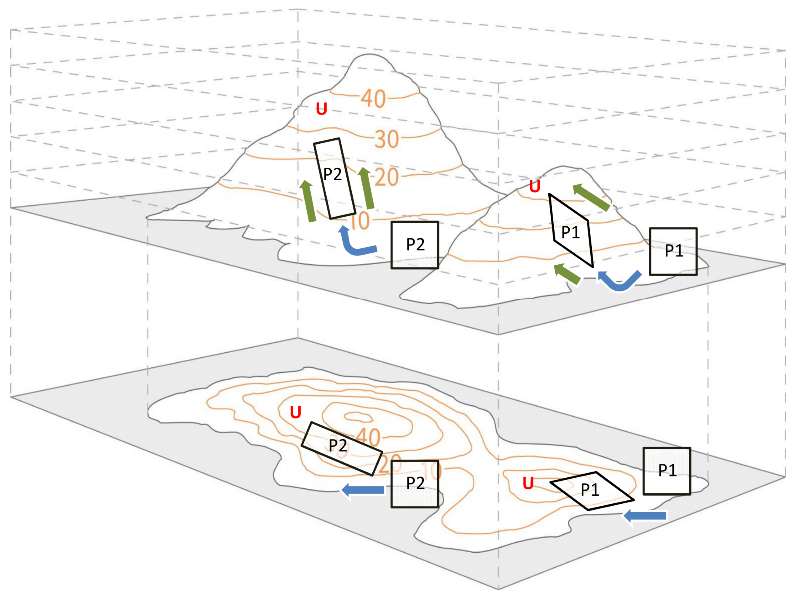
Against this backdrop, a null hypothesis is introduced and described qualitatively in Figure 1. Horizontally thin sheets of saturated air parcels contained within a near-surface layer (e.g., 0- to 2-km AGL) encounter (solid blue arrows) a dryline [7] near one or more severe thunderstorms. Parcel P1 exhibits different wind speeds along its lateral edges producing shearing effects, while parcel P2 is stretched uniformly along both sides (solid green arrows). In both instances, the parcel area and volume remain conserved quantities. As these saturated air parcels ascend the terrain (brown contours), they become tilted (see 3-D perspective in the figure) into a thunderstorm’s updraft (red “U” symbol) and developing mesocyclone. As storm reflectivity and relative velocity signatures are monitored over $\Delta t$ ≈ 2 h, falling local pressure in the supercell may signal vortex generation, warranting heightened attention and public weather alerts from meteorologists. Storm velocities of 1-km grid spacing are sufficient to capture these pressure perturbations and a mesoscyclone depth of 6-km or more [9]. This hypothesis will be tested in the four mesoscale events and described further in the following sections.

3. Materials and Methods

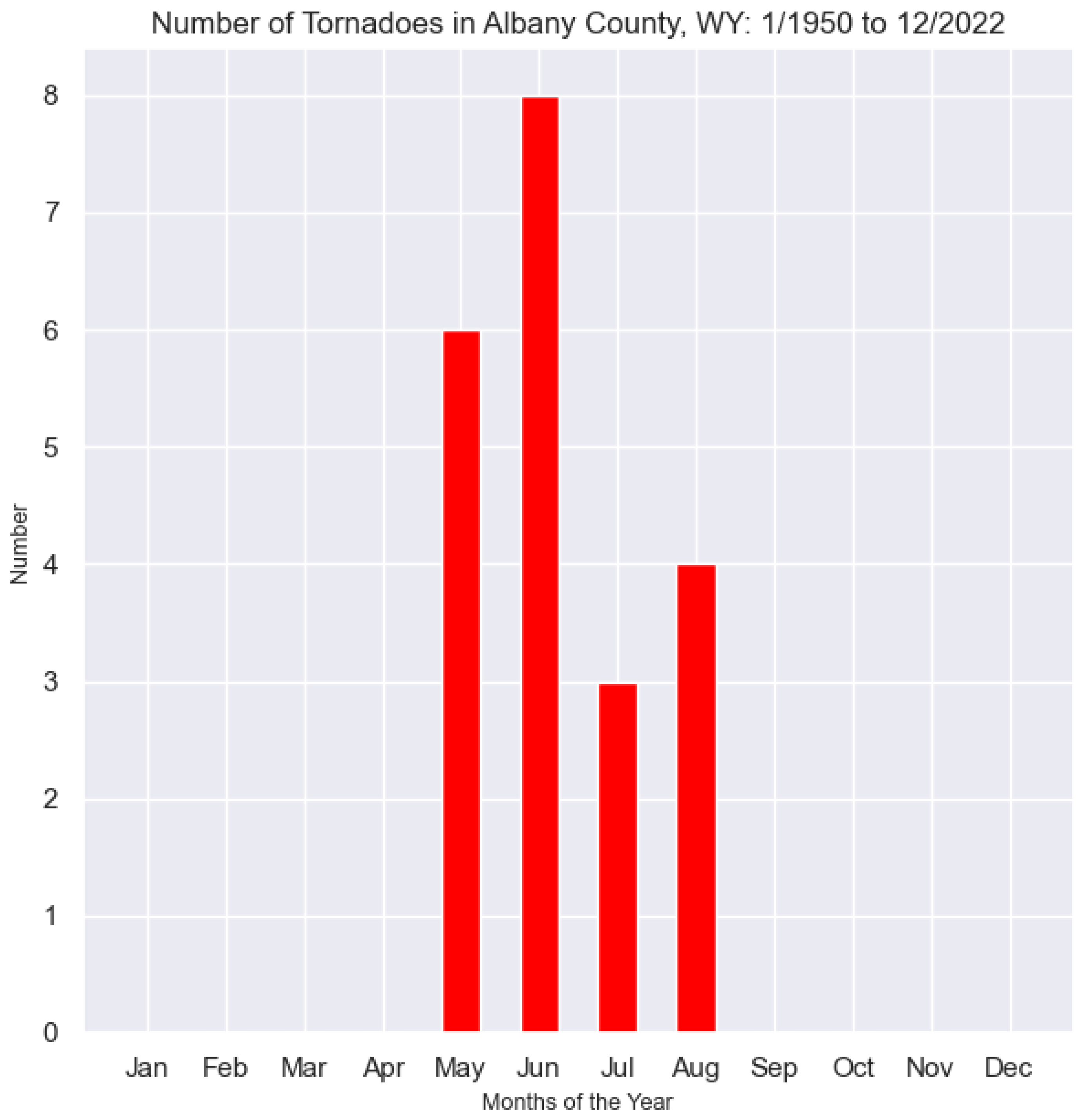
The National Centers for Environmental Information (NCEI) historical database of severe weather events indicates that Wyoming tornadoes are rare occurrences, averaging about 10 per year (January 1950 to December 2022). In particular, Figure 2 shows the monthly distribution of tornadoes for Albany County in Wyoming. The most active period is May through July (17/21 days or 81%), with no occurrences from November to March over the 72-year period. Accordingly, four cases of high-altitude moderate to severe tornadoes are explored in this study: Case A: 27 May 2018, Case B: 6 June 2018, Case C: 19 June 2018, and Case D: 6 July 2019. All events occurred between the early afternoon (1900 UTC or 100 PM MDT) and early evening (0000 UTC or 600 PM MDT) hours.

3.1. Surface Observations

The University of Utah’s MesoWest (network) repository [11] contains weather observations from multiple sensing platforms (1997 to present) for the United States. The number of surface reporting stations for the events varies from 30 to 40 sites (see Figure 3 below for details). Since there are different sources of weather observations with various reporting times, the methodology uses a rolling 1-h window to collect and store the most recent observation within that period. Mesonet observations negatively flagged by the Mesowest algorithms are completely rejected; a second pass quality control filter rechecks processed data for further errors. The raw mesonet variables include drybulb temperature, dewpoint temperature, station pressure, wind speed, and wind direction at the height (MSL) of each reporting station.

Irregularly-spaced surface observations are interpolated by an inverse distance-weight expression in a Barnes Objective Analysis to generate a $\Delta x$ ≈ $\Delta y$ ≈ 3-km grid of smoothed meteorological fields. The calculated fields from the gridded mesonet output include horizontal (u, v) wind vector, Jacobian matrix determinant of the horizontal wind, vector magnitude of the gradient of the surface dewpoint depression, horizontal divergence of the (u, v) wind, and moisture flux divergence [12]. The extrapolated mean sea-level pressure integrated over station elevation assuming a conditionally unstable environmental temperature lapse rate (8.15 °C km${}^{-1}$) and pressure drop [12] associated with inflow vortex acceleration are calculated for thunderstorm and vortex identification.

In particular, the Jacobian (J) of the horizontal wind can be mathematically written in matrix form [8] as:

$$J_{u,v}=\left[\begin{array}{cc}\frac{\partial u}{\partial x}& \frac{\partial v}{\partial y}\\ \frac{\partial v}{\partial x}& \frac{\partial u}{\partial y}\end{array}\right]$$

(1)

Solving Equation (1) further, the Jacobian matrix determinant (J) is the difference between the products of two terms describing stretching and shearing of the surface airflow:

$$J=\frac{\partial u}{\partial x}\frac{\partial v}{\partial y}-\frac{\partial u}{\partial y}\frac{\partial v}{\partial x}$$

(2)

Based on Equation (2), if J > 0, then stretching is more important than shearing effects. If J = 0, then neither forcing mechanism is dominant, but if J < 0, then shearing is more important than stretching effects.

3.2. Doppler Weather Radar Observations

The NCEI stores the National Weather Service (NWS) Weather Surveillance Radar-88 Doppler (WSR-88D) single and dual polarization data sets from 1992 to the present time for over 160 stationary weather radar acquisition towers in the United States. The KCYS radar tower (Cheyenne, WY, USA) (dark blue radar dish symbol in the lower right of Figure 3) unit conducts various weather scans of the atmosphere at multiple elevation angles and ranges. Storm evolution and motion are collected from the KCYS WSR-88D 0.5 degree angle: Long Range Base Reflectivity (N0Q) and Storm Relative (Radial) Velocity (N0S) data sets. The Long Range Reflectivity product uses a higher spatial resolution (8-bit) than the legacy single polarization reflectivity products (e.g., 4-bit N0R) with longer ranges for observing weather phenomena. It will be demonstrated that the N0Q product can detect a low-level tornado vortex signature even at ranges of 60 to 80 km from the radar. Radar beam spreading and attenuation beyond 80-km ranges mitigates useful storm identification [6].

The N0Q and N0S radar products are suitable for the region of study. The 0.5-degree beam centerline is unblocked by nearby mountains, ≈1.0 km AGL above the average terrain (2.8 km MSL) of the Laramie Range but is low enough in the atmosphere (about 1.5 km AGL above mesonet stations in the Laramie Valley) to be systematically integrated into the surface analysis. A constant altitude version of the Long Range Reflectivity product was not available in the NCEI archive for comparison. For clarity, the Storm Relative Velocity product subtracts out the storm motion of a given cell from its ground-relative motion allowing measurements of internal flow velocities. The grid spacing of the N0S product is 1 km and capable of resolving pressure perturbations associated with a mesoscyclone of 6 km or greater [9].

Accordingly, a pressure drop ($\Delta p$) associated with inflow acceleration of environmental air [12] into the center of a tornado is given by:

$$\Delta p=0.5\times \rho [v{}^2-v_{\infty }{}^2]$$

(3)

In Equation (3), v is wind speed near the storm (in this study, estimated from the absolute value of the radar-based storm relative wind speed), $v_{\infty }$ is wind speed far away from the storm (assumption: 10 m s${}^{-1}$ = 20 knots), and $\rho$ is air density of 1 kg m${}^{-3}$.

4. Topography

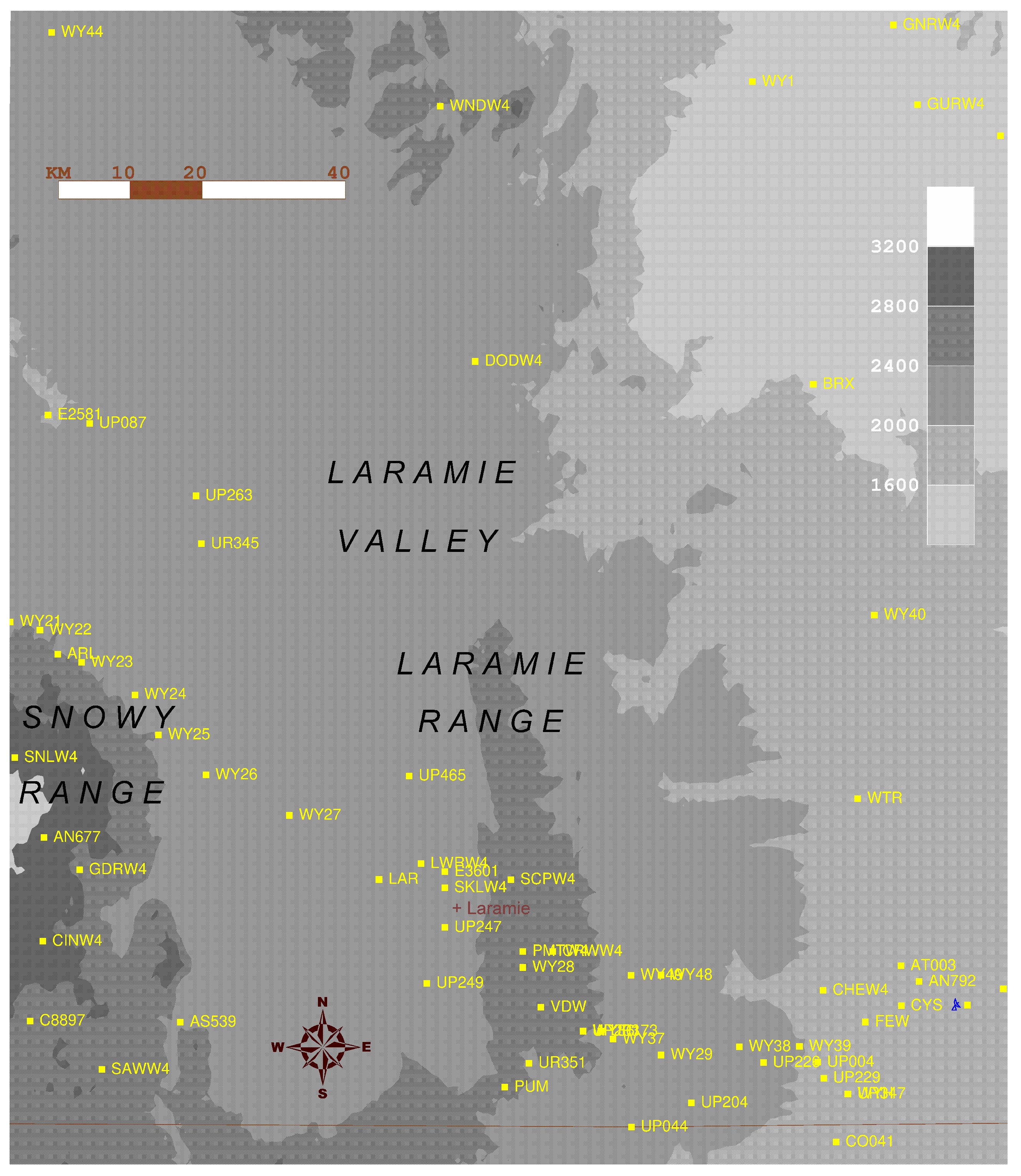
Figure 3 indicates the topography for the region of interest with several map identifiers in Albany County, Wyoming. Elevations generally rise in a north-to-south direction across the map. A network of 30–40 weather surface observations (yellow squares with labels) and a dual-polarization Doppler weather radar tower (KCYS in the lower right of the figure) provides three-dimensional weather scans of this region. A selected height interval of $\Delta z$ = 400 m delineates major differences among plains, plateaus, and mountains within the region of study. The principal orographic feature is the ≈250-km wide Laramie Valley, situated in between two large topographic barriers. The Laramie Range, in the center of the domain (≈180-km long and ≈50-km wide), is oriented meridionally with elevations from 2400 to 3000 m MSL. The Snowy Range in the western portion of the figure is situated on the west side of the valley with elevations between 2400 and 3200 m MSL. The city of Laramie (2200 m MSL) is located at the western foot of the Laramie Range; Cheyenne (1800 m MSL) (near CYS) lies ≈85 km east of Laramie within a vast high-elevation plateau of roughly 1600 to 2000 m MSL. In the northeast quadrant, the terrain gradually slopes lower and flattens out to a plain with rolling hills, decreasing in elevation from 2000 m MSL to less than 1600 m MSL. These background maps will be used in the figures of this study.

5. Results

5.1. Environmental Conditions: (t − 2) h

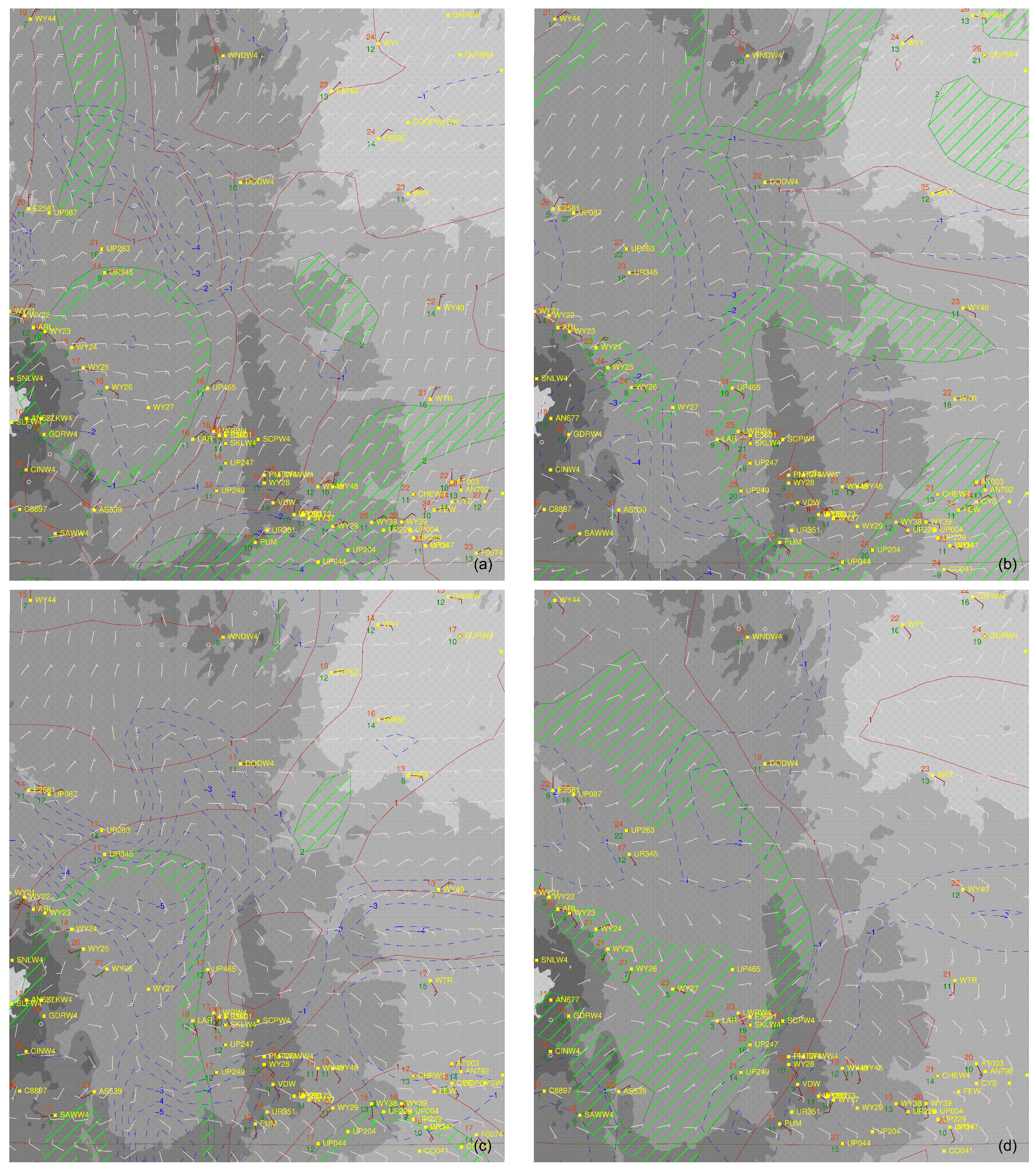
The mesoscale environment approximately two hours prior to tornado initiation is depicted in Figure 4. The dryline or dewpoint front is a leading intrusion of dry air; thunderstorms initially develop along and just east of the boundary in the nearly saturated unstable air [12]. As a first guess in the methodology, this boundary is computed as the vector magnitude of the gradient of the surface dewpoint depression [12] (+1 to +3 × ${10}^{-4}$ °C m${}^{-1}$). Contours appear as solid brown and green lines with slanted green regions representing higher relative humidities (smaller dewpoint depressions). In all the events, a dryline with variable symmetry is generally situated in the middle of the domain. Cases B and D show curvilinear meridional boundaries, while the other two cases display more discontinuous serpentine configurations. A common spatial pattern also emerges in the extrapolated horizontal wind field. The surface divergence of the interpolated 3-km horizontal wind field (dashed blue contours) is strongly negative, indicating low-level convergence with maximum vertical lift along the boundary, especially in the Laramie Valley. The strongest convergence is centered northwest or west of the Laramie Range.

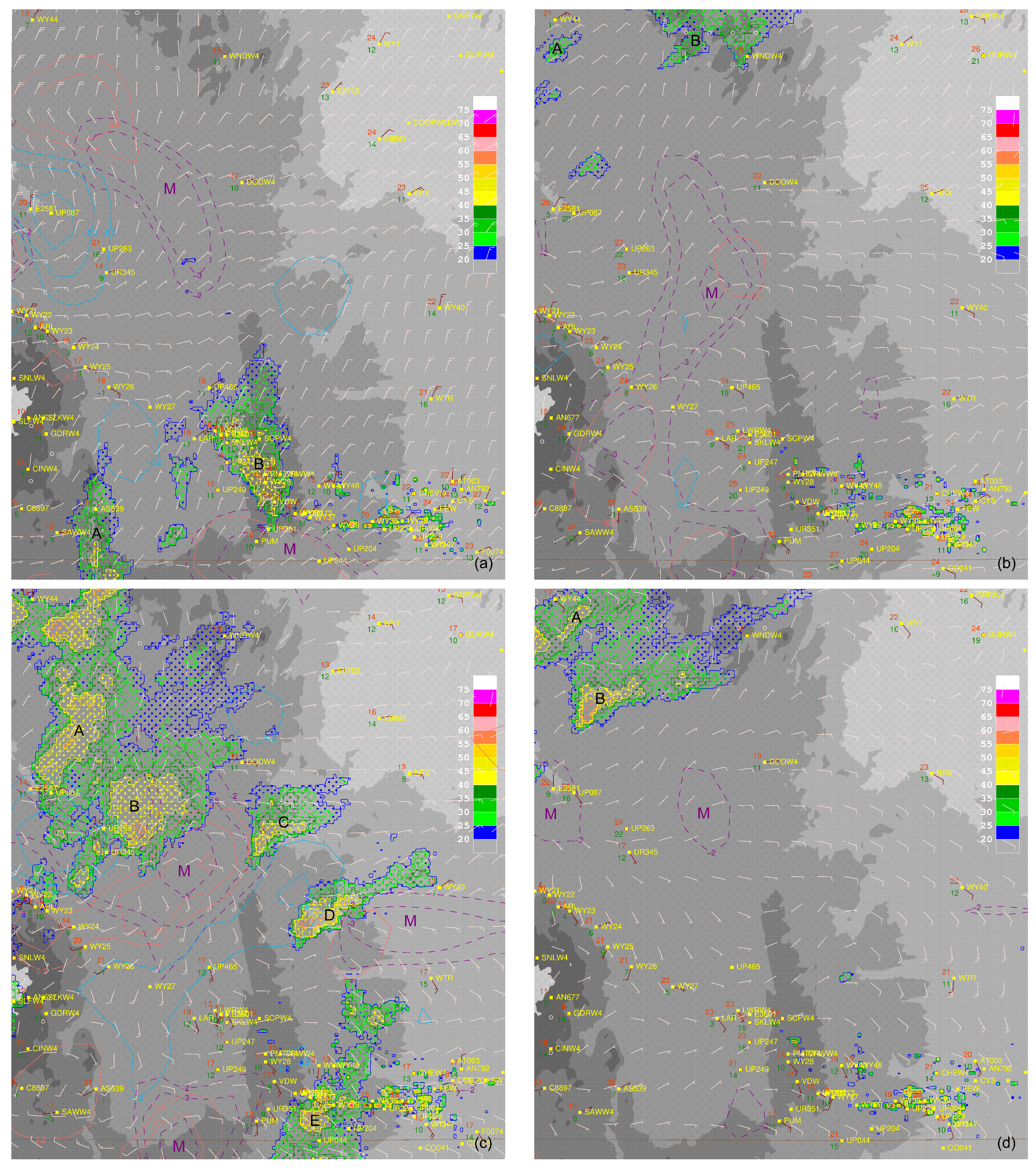
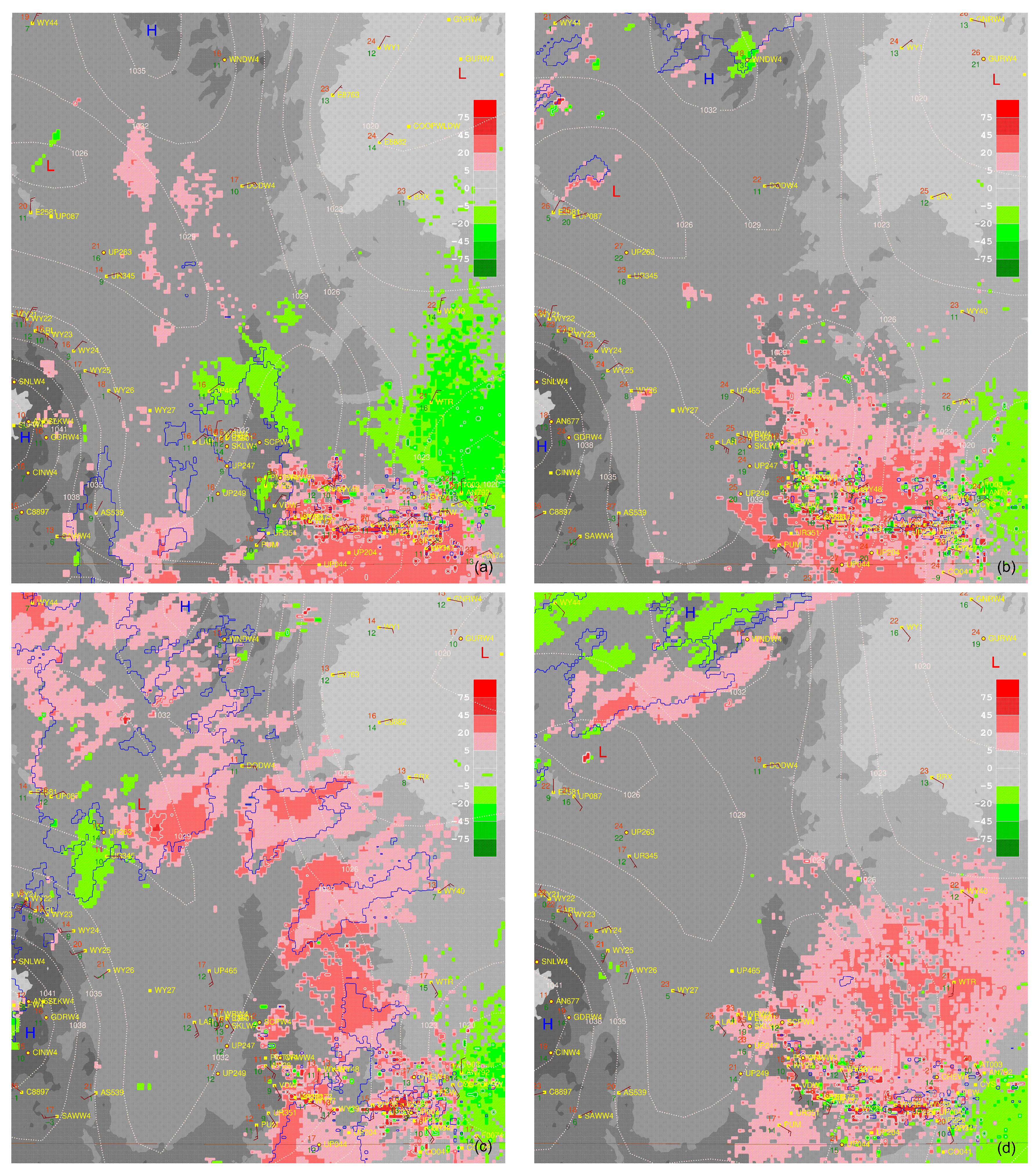
Figure 5 (long range base reflectivity) and Figure 6 (storm relative velocity) capture the initial storm environments for each case. The dewpoint depression and divergence analysis in Figure 4 is assimilated into surface moisture flux divergence computed from station dewpoint temperature, pressure, and horizontal wind (Figure 5). The negative values in Figure 5 are dashed purple contours indicating horizontal low-level negative divergence or convergence of saturated air and implied vertical ascent consistent with mass continuity [12]. In Figure 5, locations with the strongest moisture flux convergence associated with dryline segments are highlighted by purple “M” symbols. The thunderstorm identifiers are indicated by black labels in the figure.

A strikingly similar pattern is evident in the four tornadic episodes. In Figure 5, scattered showers and thunderstorms form on the northwest and west sides near moisture convergence maxima in the Laramie Valley. With the exception of Case C, convection is generally isolated to scattered in areal coverage, at first, with light to moderate intensity (20 to 45 dBZ). There are four intense cells in Case C within a large region of flow shearing (J < 0: solid blue contours). In Figure 6, the general pressure pattern features high pressure along the Snowy Range with a sharp trough of lower pressures in the Laramie Valley and extending southward along the higher terrain of the Laramie Range. This pressure pattern remained relatively stationary and persisted for the next two hours.

5.2. Supercell Thunderstorm Formation: (t − 1) h

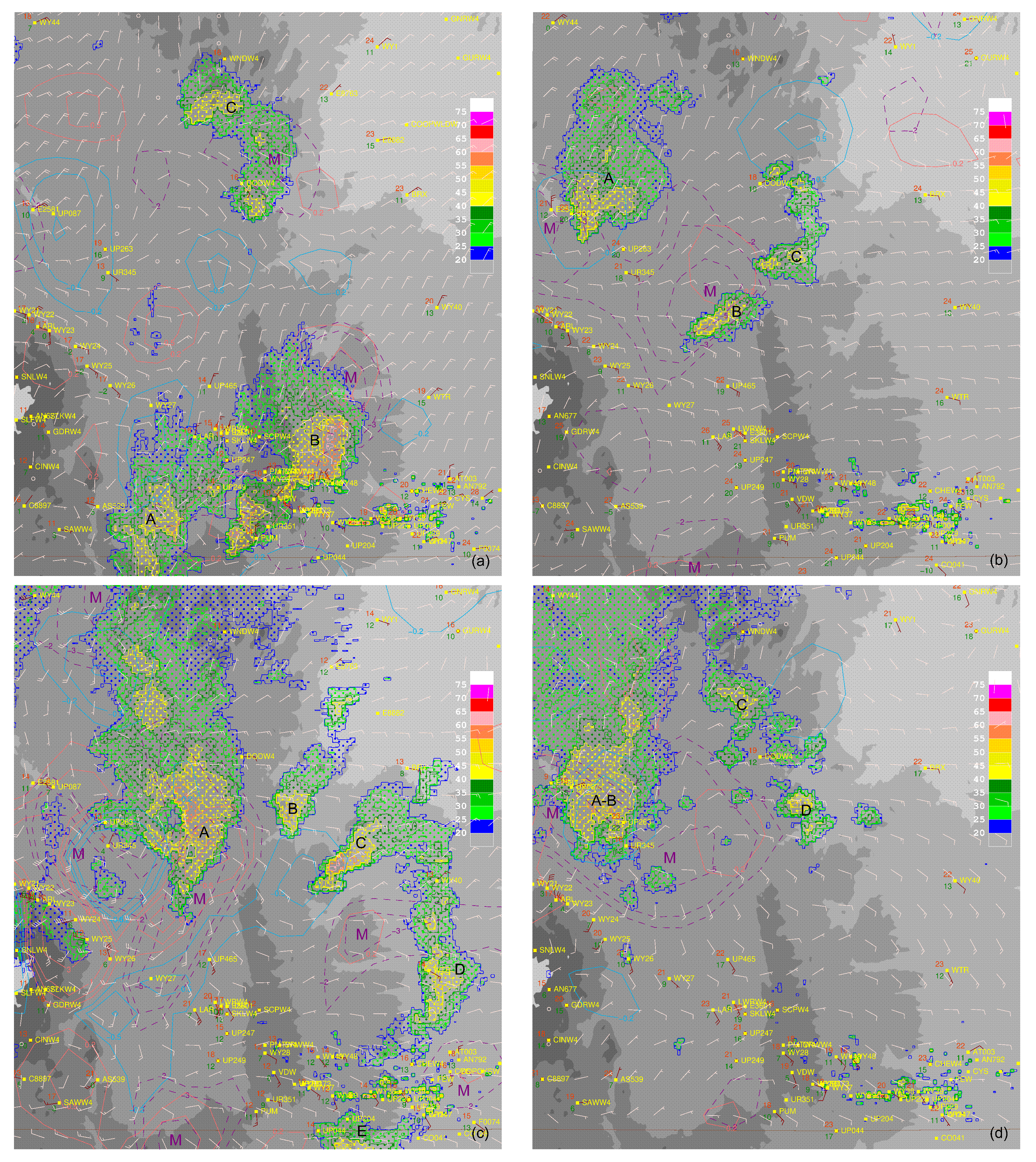
Figure 7 and Figure 8 depict the storm environments at roughly 1 h prior to tornado formation with low-level (0.5 degrees) radar scans of long-range base reflectivity and storm relative velocity. As compared to an hour ago, the convection is more widespread and severe, organized into larger isolated cells and lines of moderate to heavy intensity (35 to 55 dBZ) in the unstable saturated air. These patterns mark the supercell thunderstorm phase of the heuristic analysis. Structurally, negative and positive Jacobian regions are superimposed with moisture flux divergence minima coincident with thunderstorm updrafts.

In particular, in Case A, lines of severe thunderstorms (cells A, B, and C) form in the upper and lower Laramie Valley. Several areas of negative Jacobian determinant (solid blue contours) delineate areas of low-level flow shearing near all the thunderstorms in Figure 7. Case B shows three distinct large convective cells in the Laramie Valley with adjacent areas of flow shearing. In Case C, the convection is more widespread in a large semi-circular arc of discontinuous cells A, B, C, D, and E along the periphery of a well-defined moisture flux convergence axis (purple “M” symbols). Although not as apparent in the other events, the largest storm in cell A exhibits a prominent inflow of stretched air (positive Jacobian determinant: solid orange contours) along the west and east sides of the storm. In Case D, there is a large single merged cell (A-B) with weaker and smaller isolated strong convection (storms C and D) east of it. Figure 8 shows the stationary pressure trough in the Laramie Valley with local pressure falls (solid white contours) near each of the cells suggesting possible vortex formation. These parcels of stretched and sheared saturated air are lifted along the dryline segments towards the updrafts of the thunderstorms.

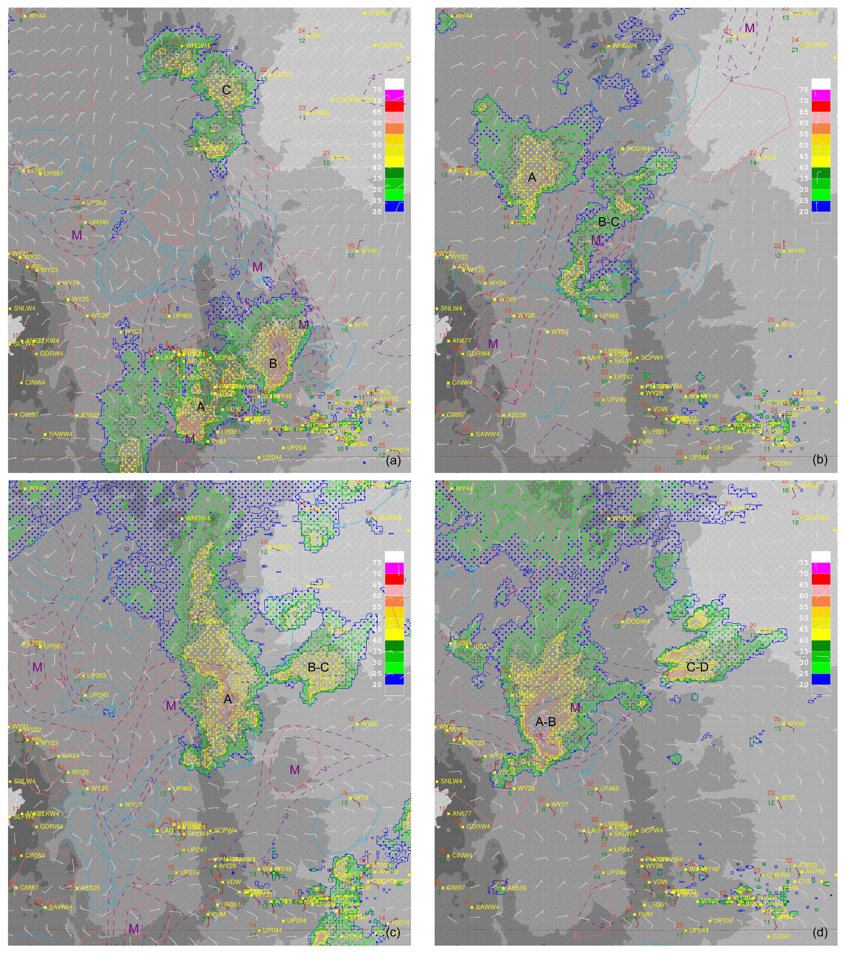
5.3. Tornado Formation: (t − 5) min

Figure 9 indicates the low-level (0.5 degrees) scans of long-range radar reflectivity just prior to tornado touchdowns as verified from weather spotter reports and radar signatures for the events. At first inspection, intense thunderstorms occur in nearly adjacent pairs for each event. However, a more significant pattern of couplets is evident– flow stretching (positive Jacobian determinant: solid orange contours) and shearing (negative Jacobian determinant: solid blue contours) circumscribe each (labeled) supercell thunderstorm and a low-level “hook echo” signature suggesting updraft locations and possible tornadic rotation [12]. These kinematic effects occur at strong moisture flux convergence axes (purple “M” symbols) along the dryline in the unstable air mass. Geographically, this conspicuous pattern of flow stretching and shearing is situated on the west (back) and east (front) sides of each severe storm, respectively.

For example, in Case A, cell B shows an easterly inflow along a moisture boundary and shearing region on its eastern side near a hook echo signature signifying a tornado vortex [12]. The region of shearing just southwest of mesonet station WTR is lifted topographically approximately 0.8 km AGL into the thunderstorm’s updraft. The severe thunderstorms in Case B are oriented near a strong moisture flux convergence axis (purple “M” symbols) associated with shearing and stretching regions. Cell A contains a prominent hook echo along its southern flank just northeast of station UR345. Intense cells B and C merge into one large curvilinear echo region with well-defined shearing and stretching regions. A large double-bean-shaped echo denoting at least one possible tornado vortex is situated on the southern terminus of the storm near UP465. The salient moisture flux convergence axis defining a segment of the dryline extends diagonally from in between cells A and B-C to the eastern edge of the Snowy Range. In the eastern part of storm B-C, there is a well-defined sickle-shaped region of flow shearing (J < 0: solid blue contours) from mesonet stations DODW4 to UP465; the low-level southeasterly flow is lifted, tilted topographically roughly 1.2 km AGL, and ascends into the updraft. Case C is similar to Case B, with a single large cell A and cell merger (B-C) east of it. Storm A is the largest and most intense of the convection, with a hook echo evident on the southern flank of the storm northeast of station UP465. Once more, the low-level easterly flow is lifted over the terrain (≈0.4 km AGL) into the updraft zone associated with a hook echo. In Case D, cells A and B merge into a larger storm cluster. The moisture convergence axis in cells A-B is superimposed with flow shearing, then lifted over the higher terrain (about 1.2 km AGL) into the thunderstorm’s updraft as a hook echo forms north of station UP465. Further east, cells C and D merge into a larger cell which contains weaker stretching and shearing flow patterns. These results demonstrate the mechanisms described in Figure 1.

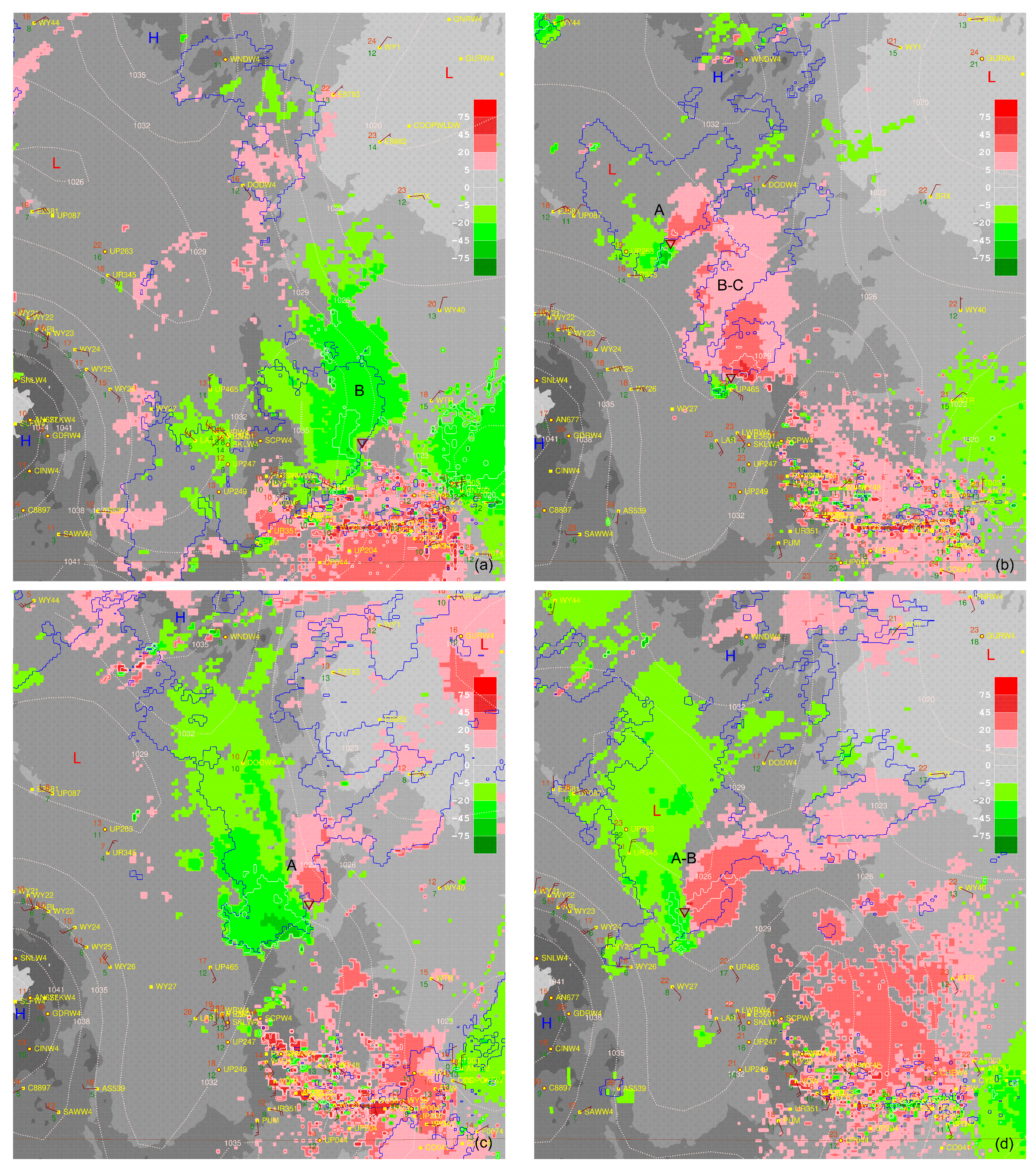
For further evidence of vortex detection, Figure 10 indicates the 0.5 degrees scan of storm relative velocity just prior to tornado touchdowns for the events. The outline of the 20 dBZ echo (dark blue) locates each (labeled) severe storm. In each case, storm pressure falls of 1 to 3 hPa (solid white contours) lie in between inbound (green) and outbound (red) radial winds, a velocity pattern of cyclonic rotation [6]. This intersection of the velocity couplets and pressure drops suggests the actual vortex locations (upside-down dark brown triangles in the figure). The Enhanced Fujita (EF) Scale rates tornado intensity as a function of potential wind (speed) damages [13]. Furthermore, observed gate-to-gate wind speed shear (gws) normal to radial velocity couplets (Figure 10) describes the EF storm classifications for the events. For instance, in Case A, cell B shows a tornado (EF2) where gws ≈ 100 knots. In Case B, cell A develops an EF1 tornado with strong gws≈ 90 knots while merged cell B-C contains the large hook echo with an intense (EF3) tornado exhibiting gate-to-gate wind speed shear of over 130 knots, the most severe vortex in all the events. Case C contains a well-defined tornado (cell A) with strong gws≈ 80 knots (EF1). Likewise, Case D shows a prominent hook echo (storm A-B) with a large region of stretched flow into the updraft zone coincident with a strong gws≈ 80 knots (EF1).

6. Discussion

The next goal is to develop an experimental conditional probability [10,14] associated with the null hypothesis, namely, that the intersection of the Jacobian determinant and moisture flux convergence within a thunderstorm updraft may signal tornadogenesis. These physical processes are independent of each other, so their joint probabilities can be multiplied together [14].

Hence, expressing Bayes’ theorem in the general hypothesis form [10]:

$$P(H\mid D)=P(D\mid H)\times P\left(H\right)/P\left(D\right)$$

(4)

$P(H\mid D)$ is the posterior (conditional) probability of the hypothesis given the data has occurred, $P(D\mid H)$ is the likelihood (conditional) probability of the data given the hypothesis has occurred, $P\left(H\right)$ is the prior probability of the hypothesis with two possible outcomes, and $P\left(D\right)$ is the prior probability of the data regardless of the hypothesis and is the total probability of all outcomes.

For this study, substituting for each of the above terms and splitting the Jacobian determinant matrix into airflow stretching and shearing probabilities yields:

$$P(D\mid H)=0.81$$

(5)

and for shearing effects,

$$P\left(H\right)=P(J<0)\times P(M<0)$$

(6)

or for stretching effects,

$$P\left(H\right)=P(J>0)\times P(M<0)$$

(7)

and (total probability),

$$P\left(D\right)=\left[P\right(J<0)\times P(M<0)+P(J>0)\times P(M<0\left)\right]$$

(8)

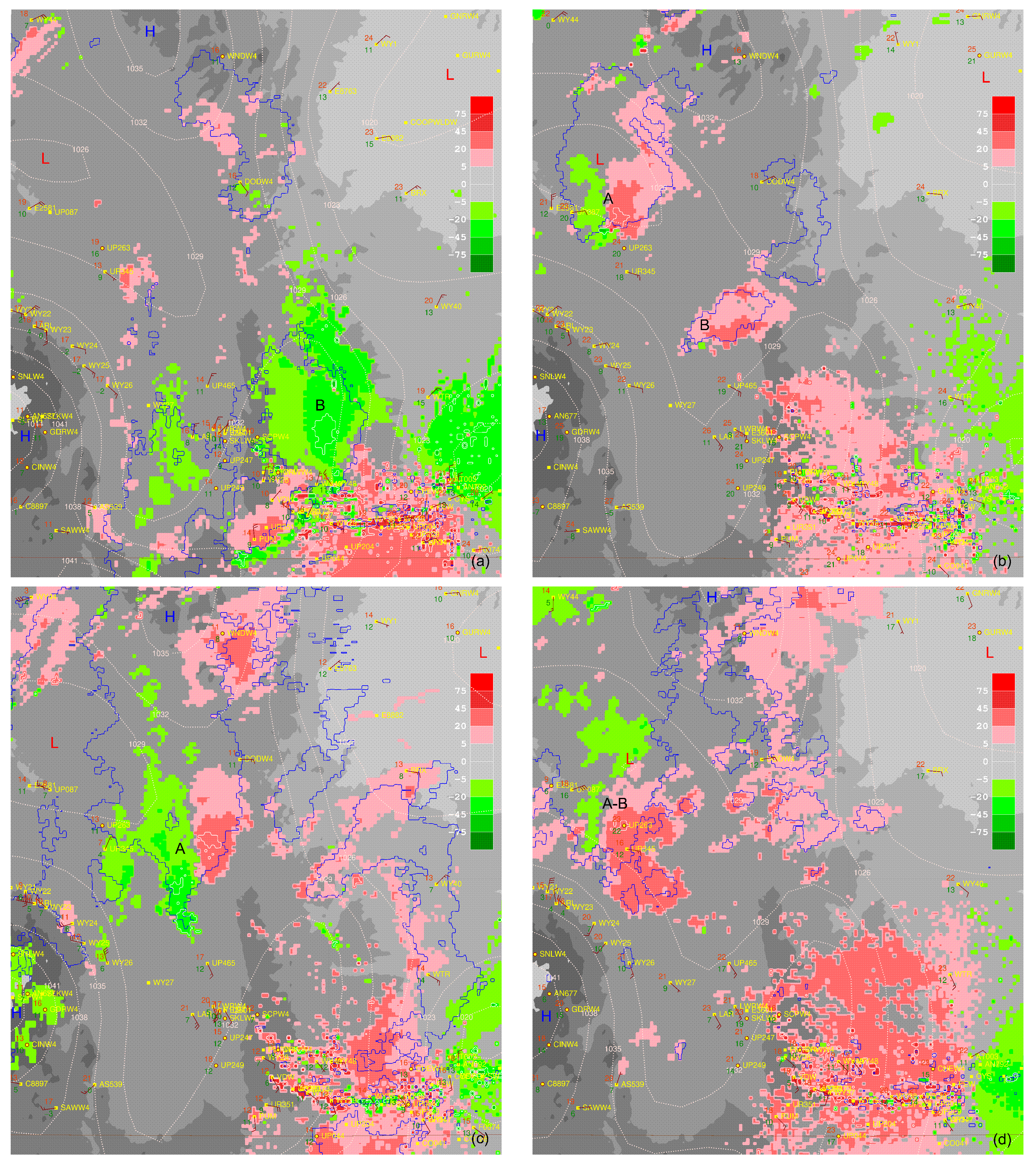
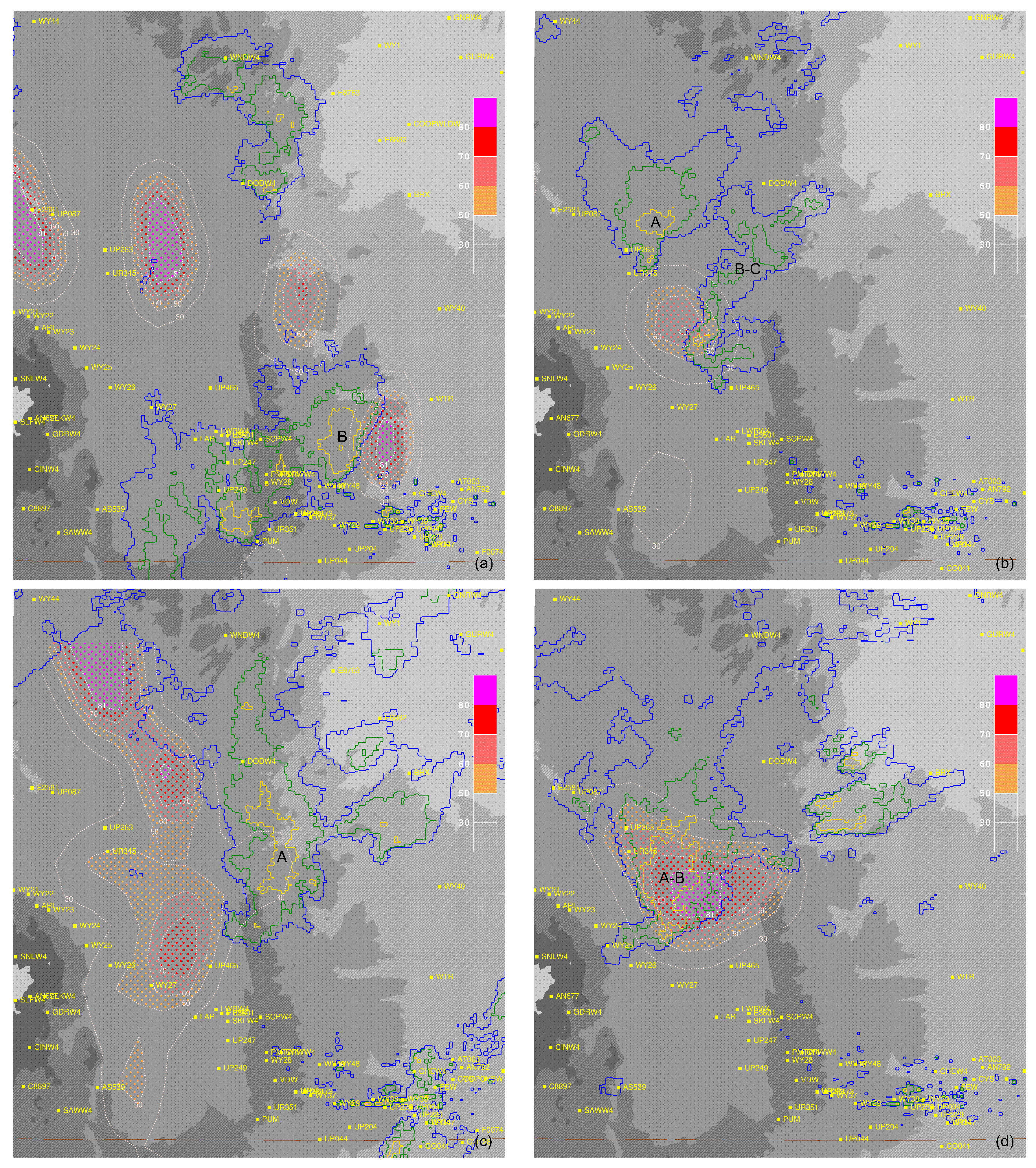
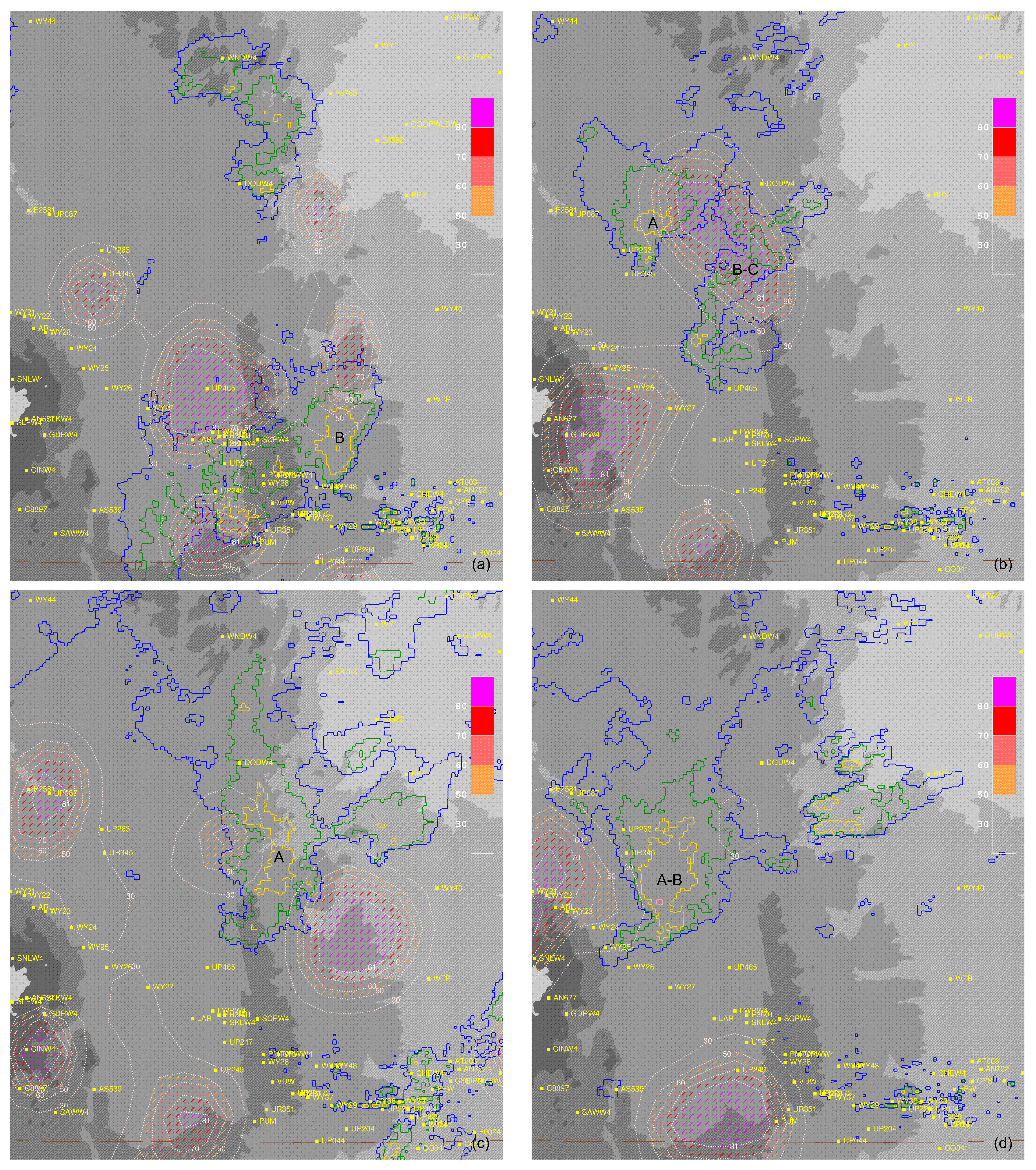
Figure 11 (Equation (6)) and Figure 12 (Equation (7)) show the Bayesian posterior probabilities related to shearing and stretching effects just prior to tornado touchdowns for each case. Storm identifiers associated with tornadoes are labeled with black capital letters. This posterior total probability in Equation (8) consists of the sum of terms related to stretching and shearing of the airflow. An assumption is that this probability is capped at 0.81 (Equation (5)), reflecting an upper limit to this estimate based on the seasonal storm climatology for Albany County, Wyoming (Figure 2). There is a general pattern of 30 to 80% posterior probability for all the events. In Case A, storm B contains a blend of stretching and shearing posterior probabilities totaling 70%. In Case B, cell A is dominated by stretching effects with a 70 to 80% posterior probability, notably in the eastern part of the storm. Cell B-C is influenced by flow stretching, but its hook echo in the southern part of the storm is more influenced by shearing effects. In Case C, cell A contains a 30 to 50% posterior probability of vortex detection associated with stretching effects. In Case D, there is a large elliptical area of 70 to 80% posterior probability in storm A-B due to the shearing of the airflow. These results suggest sufficient evidence to accept the null hypothesis.

7. Conclusions

Forecasting tornadoes presents many challenges requiring different solutions, including direct manual observations, climatological maps of precursor synoptic conditions, complex four-dimensional numerical model simulations, and automated machine learning algorithms. These challenges are magnified even further over the complex terrain of the Intermountain United States in geographical regions like Wyoming. Consequently, a complimentary and novel heuristic methodology featuring Bayes’ theorem was presented to help meteorologists detect tornadoes from supercell thunderstorms in the complex terrain of southern Wyoming. These events occurred on 27 May 2018, 6 June 2018, 19 June 2018, and 6 July 2019 in Albany County, Wyoming.

Among the shortcuts, rules-of-thumb, and assumptions illuminating the tested null hypothesis, the surface predictors included moisture convergence axes associated with dryline segments and the Jacobian determinant of the horizontal wind illustrating flow shearing and stretching into the updrafts of these storms. Observational evidence obtained from surface and radar sources suggested Bayesian posterior probabilities of 30 to 80 percent associated with vortex detection in the events. Hopefully, similar studies using heuristic and Bayesian principles will produce positive results for other mountain-valley systems in the United States and the world.

References

- Fujita, T.T. The Teton-Yellowstone tornado of 21 July 1987. Mon. Weather Rev. 1989, 117, 1913–1940. [Google Scholar] [CrossRef]
- Evenson, E.C.; Johns, R.H. Some climatological and synoptic aspects of severe weather development in the northwestern United States. Natl. Weather Dig. 1996, 20, 34–50. [Google Scholar]
- Andretta, T.A.; Wojcik, W.A.; Simosko, K. Climatological synoptic patterns of tornado genesis in eastern Idaho. Natl. Weather Assoc. Electron. J. Oper. Meteorol. 2004, 5, 1–69. [Google Scholar]
- Wakimoto, R.M.; Atkins, N.T.; Wurman, J. The LaGrange tornado during VORTEX2. Part I: Photogrammetric analysis of the tornado combined with single-Doppler radar data. Mon. Weather Rev. 2011, 139, 2233–2258. [Google Scholar] [CrossRef]
- Atkins, N.T.; McGee, A.; Ducharme, R.; Wakimoto, R.M.; Wurman, J. The LaGrange tornado during VORTEX2. Part II: Photogrammetric analysis of the tornado combined with dual-Doppler radar data. Mon. Weather Rev. 2012, 140, 2939–2958. [Google Scholar] [CrossRef]
- Brooks, H.; Correia, J. Long-term performance metrics for National Weather Service tornado warnings. Weather Forecast. 2018, 33, 1501–1511. [Google Scholar] [CrossRef]
- Geerts, B.; Andretta, T.; Luberda, S.; Vogt, J.; Wang, Y.; Oolman, L.D.; Finch, J.; Bikos, D. A case study of a long-lived tornadic mesocyclone in a low-CAPE complex-terrain environment. Electron. J. Sev. Storms Meteorol. 2009, 4, 1–29. [Google Scholar] [CrossRef]
- Snook, N.; Xue, M.; Jung, Y. Tornado-resolving ensemble and probabilistic predictions of the 20 May 2013 Newcastle–Moore EF5 tornado. Mon. Weather Rev. 2019, 147, 1215–1235. [Google Scholar] [CrossRef]
- Lagerquist, R.; McGovern, A.; Homeyer, C.R.; Gagne, D.J., II; Smith, T. Deep learning on three-dimensional multiscale data for next-hour tornado prediction. Mon. Weather Rev. 2020, 148, 2837–2861. [Google Scholar] [CrossRef]
- Doswell, C.A., III. Weather forecasting by humans—Heuristics and decision-making. Weather Forecast. 2004, 19, 1115–1126. [Google Scholar] [CrossRef]
- Horel, J.; Splitt, M.; Dunn, L.; Pechmann, J.; White, B.; Ciliberti, C.; Lazarus, S.; Slemmer, J.; Zaff, D.; Burks, J. Mesowest: Cooperative mesonets in the western United States. Bull. Am. Meteorol. Soc. 2002, 83, 211–225. [Google Scholar] [CrossRef]
- Markowski, P.; Richardson, Y. Mesoscale Meteorology in Midlatitudes; Wiley-Blackwell: Oxford, UK, 2013; 430p. [Google Scholar]
- Edwards, R.; LaDue, J.G.; Ferree, J.T.; Scharfenberg, K.; Maier, C.; Coulbourne, W.L. Tornado intensity estimation: Past, present, and future. Bull. Am. Meteorol. Soc. 2013, 94, 641–653. [Google Scholar] [CrossRef]
- Wilks, D.S. Statistical Methods in Atmospheric Sciences; Academic Press: San Diego, CA, USA, 1995; 464p. [Google Scholar]
Figure 1.
Schematic of hypothesis illustrating the interaction of saturated air parcels and environmental wind flow over modeled complex terrain with a thunderstorm updraft from 2-D (bottom graphic) and 3-D (top graphic) perspectives: elevation contours (solid brown lines), air parcels (P1, P2), thunderstorm updraft (red “U” symbol), ambient wind flow (solid green arrows) affecting parcels, and parcel motion over time (solid blue arrows).
Figure 2.
Monthly distribution of tornadoes in Albany County, Wyoming from January 1950 to December 2022.
Figure 3.
Topography of southern Wyoming including Albany County with black geographical labels for various regions, distance legend, compass heading, and terrain elevation key (grey tones: m MSL). Mesonet identifiers are indicated by yellow squares with labels in the domain. The brown horizontal line at the bottom of the figure is the Wyoming-Colorado border. The city of Laramie (dark brown cross symbol and label) is situated at the western foot of the Laramie Range. The WSR-88D KCYS radar tower (dark blue radar dish symbol) is located just east of mesonet station, CYS.
Figure 4.
Dryline boundary computed as the vector magnitude of the gradient of the surface dewpoint depression (solid brown and green lines with slanted green regions for higher relative humidities) ( °C m) and surface divergence of the horizontal (u, v) wind (dashed blue contours) ( s) for Cases (a) A at 2000 UTC, (b) B at 2203 UTC, (c) C at 1902 UTC, and (d) D at 2200 UTC.
Figure 5.
WSR-88D KCYS N0Q (Long Range Base Reflectivity at 0.5 degrees) (dBZ) (dotted color table from 20 (dark blue) to 75 (white) dBZ), surface moisture flux divergence ( g kg m s) (negative: purple dashed contours with “M” symbols for local minima), Jacobian matrix determinant ( s) (negative: solid blue and positive: solid orange contours), surface observations (red: drybulb temperature (°C), dark green: dewpoint temperature (°C), 10-m AGL wind barbs (brown: every 5 knots), and 3-km interpolated 10-m AGL wind vectors (vanilla: every 5 knots)) for Cases (a) A at 2000 UTC, (b) B at 2203 UTC, (c) C at 1902 UTC, and (d) D at 2200 UTC. Storm identifiers are labeled with black capital letters (e.g., “A”, “B”, “C”, “D”, or “E”).
Figure 6.
WSR-88D KCYS N0S (Storm Relative Velocity at 0.5 degrees) (knots) (solid color table from −75 (inbound green) to +75 (outbound red) knots), extrapolated mean sea-level pressure (hPa: dotted vanilla contours), and surface observations (red: drybulb temperature (°C), dark green: dewpoint temperature (°C), and 10-m AGL wind barbs (brown: every 5 knots)) for Cases (a) A at 2000 UTC, (b) B at 2203 UTC, (c) C at 1902 UTC, and (d) D at 2200 UTC. The outline of the 20 dBZ echo is a dark blue contour. Locations of high and low air pressure extrema are indicated by blue “H” and red “L” symbols, respectively.
Figure 7.
Same data as in Figure 5 but for Cases (a) A at 2100 UTC, (b) B at 2302 UTC, (c) C at 1930 UTC, and (d) D at 2330 UTC. Storm identifiers are labeled with black capital letters.
Figure 8.
Same data as in Figure 6 but for Cases (a) A at 2100 UTC, (b) B at 2302 UTC, (c) C at 1930 UTC, and (d) D at 2330 UTC. Storm identifiers are labeled with black capital letters.
Figure 9.
Same data as in Figure 5 but for Cases (a) A at 2116 UTC, (b) B at 2340 UTC, (c) C at 2003 UTC, and (d) D at 0003 UTC (next day). Storm identifiers are labeled with black capital letters.
Figure 10.
Same data as in Figure 6 but for Cases (a) A at 2116 UTC, (b) B at 2340 UTC, (c) C at 2003 UTC, and (d) D at 0003 UTC (next day). Storm identifiers associated with tornadoes are labeled with black capital letters; tornado vortexes are marked by upside-down dark brown triangles. The pressure drop associated with storm inflow acceleration is solid white contours at 1 and 3 hPa intervals and indicates the vortex location.
Figure 11.
Bayesian posterior probability (smoothed) due to shearing effects (%) of a tornado based on the negative (dotted vanilla and filled dotted colored contours) Jacobian determinant and moisture flux divergence for Cases (a) A at 2116 UTC, (b) B at 2340 UTC, (c) C at 2003 UTC, and (d) D at 0003 UTC (next day). Storm identifiers associated with tornadoes are labeled with black capital letters. Outlines of 20, 35, 50, and 65 dBZ echoes are indicated by dark blue, dark green, dark yellow, and light red contours, respectively.
Figure 12.
Bayesian posterior probability (smoothed) due to stretching effects (%) of a tornado based on the positive (dotted vanilla and filled dashed colored contours) Jacobian determinant and moisture flux divergence for Cases (a) A at 2116 UTC, (b) B at 2340 UTC, (c) C at 2003 UTC, and (d) D at 0003 UTC (next day). Storm identifiers associated with tornadoes are labeled with black capital letters. Outlines of 20, 35, 50, and 65 dBZ echoes are indicated by dark blue, dark green, dark yellow, and light red contours, respectively.
Disclaimer/Publisher’s Note: The statements, opinions and data contained in all publications are solely those of the individual author(s) and contributor(s) and not of MDPI and/or the editor(s). MDPI and/or the editor(s) disclaim responsibility for any injury to people or property resulting from any ideas, methods, instructions or products referred to in the content. |
© 2023 by the author. Licensee MDPI, Basel, Switzerland. This article is an open access article distributed under the terms and conditions of the Creative Commons Attribution (CC BY) license (https://creativecommons.org/licenses/by/4.0/).
Share and Cite
MDPI and ACS Style
Andretta, T.A. Heuristic and Bayesian Tornado Prediction in Complex Terrain of Southern Wyoming. Meteorology 2023, 2, 239-256. https://doi.org/10.3390/meteorology2020015
AMA Style
Andretta TA. Heuristic and Bayesian Tornado Prediction in Complex Terrain of Southern Wyoming. Meteorology. 2023; 2(2):239-256. https://doi.org/10.3390/meteorology2020015
Chicago/Turabian StyleAndretta, Thomas A. 2023. "Heuristic and Bayesian Tornado Prediction in Complex Terrain of Southern Wyoming" Meteorology 2, no. 2: 239-256. https://doi.org/10.3390/meteorology2020015