

Barotropic Instability during Eyewall Replacement

Abstract
:1. Introduction
2. Linear Stability Analysis
2.1. Review of the Rayleigh and Fjørtoft Conditions
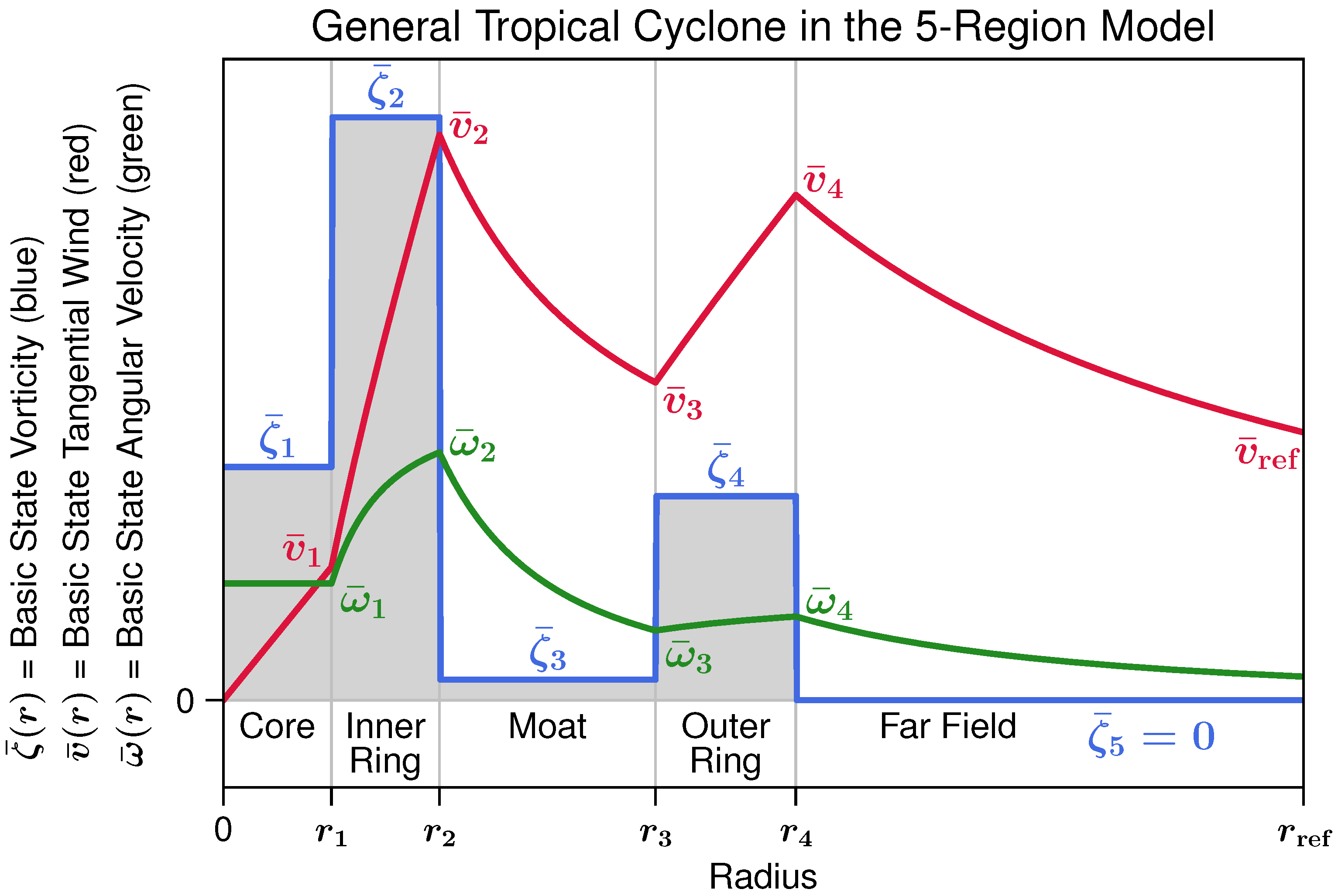
2.2. Five-Region Model
2.3. Energetics of the Linear Dynamics
3. Non-Linear Simulation of Barotropic Instability across the Moat
4. Concluding Remarks
Supplementary Materials
Author Contributions
Funding
Data Availability Statement
Acknowledgments
Conflicts of Interest
Appendix A. Model Initial Condition
References
- Willoughby, H.E.; Clos, J.A.; Shoreibah, M.G. Concentric eye walls, secondary wind maxima, and the evolution of the hurricane vortex. J. Atmos. Sci. 1982, 39, 395–411. [Google Scholar] [CrossRef]
- Black, M.L.; Willoughby, H.E. The concentric eyewall cycle of Hurricane Gilbert. Mon. Weather Rev. 1992, 120, 947–957. [Google Scholar] [CrossRef]
- Samsury, C.E.; Zipser, E.J. Secondary wind maxima in hurricanes: Airflow and relationship to rainbands. Mon. Weather Rev. 1995, 123, 3502–3517. [Google Scholar] [CrossRef]
- Dodge, P.; Burpee, R.W.; Marks, F.D., Jr. The kinematic structure of a hurricane with sea level pressure less than 900 mb. Mon. Weather Rev. 1999, 127, 987–1004. [Google Scholar] [CrossRef]
- Rozoff, C.M.; Schubert, W.H.; Kossin, J.P. Some dynamical aspects of tropical cyclone concentric eyewalls. Q. J. R. Meteorol. Soc. 2008, 134, 583–593. [Google Scholar] [CrossRef]
- Molinari, J.; Zhang, J.A.; Rogers, R.F.; Vollaro, D. Repeated eyewall replacement cycles in Hurricane Frances (2004). Mon. Weather Rev. 2019, 147, 2009–2022. [Google Scholar] [CrossRef]
- Houze, R.A., Jr.; Chen, S.S.; Smull, B.F.; Lee, W.C.; Bell, M.M. Hurricane intensity and eyewall replacement. Science 2007, 315, 1235–1239. [Google Scholar] [CrossRef]
- Hence, D.A.; Houze, R.A., Jr. Kinematic structure of convective-scale elements in the rainbands of Hurricanes Katrina and Rita (2005). J. Geophys. Res. 2008, 113, D15108. [Google Scholar] [CrossRef]
- Judt, F.; Chen, S.S. Convectively generated potential vorticity in rainbands and formation of the secondary eyewall in Hurricane Rita of 2005. J. Atmos. Sci. 2010, 67, 3581–3599. [Google Scholar] [CrossRef]
- Didlake, A.C., Jr.; Houze, R.A., Jr. Kinematics of the secondary eyewall observed in Hurricane Rita (2005). J. Atmos. Sci. 2011, 68, 1620–1636. [Google Scholar] [CrossRef]
- Bell, M.M.; Montgomery, M.T.; Lee, W.C. An axisymmetric view of concentric eyewall evolution in Hurricane Rita (2005). J. Atmos. Sci. 2012, 69, 2414–2432. [Google Scholar] [CrossRef]
- Menelaou, K.; Yau, M.K.; Martinez, Y. On the dynamics of the secondary eyewall genesis in Hurricane Wilma (2005). Geophys. Res. Lett. 2012, 39, L04801. [Google Scholar] [CrossRef]
- Didlake, A.C., Jr.; Heymsfield, G.M.; Reasor, P.D.; Guimond, S.R. Concentric eyewall asymmetries in Hurricane Gonzalo (2014) observed by airborne radar. Mon. Weather Rev. 2017, 145, 729–749. [Google Scholar] [CrossRef]
- Cha, T.Y.; Bell, M.M. Comparison of single-Doppler and multiple-Doppler wind retrievals in Hurricane Matthew (2016). Atmos. Meas. Tech. 2021, 14, 3523–3539. [Google Scholar] [CrossRef]
- Shapiro, L.J.; Willoughby, H.E. The response of balanced hurricanes to local sources of heat and momentum. J. Atmos. Sci. 1982, 39, 378–394. [Google Scholar] [CrossRef]
- Nong, S.; Emanuel, K. A numerical study of the genesis of concentric eyewalls in hurricanes. Q. J. R. Meteorol. Soc. 2003, 129, 3323–3338. [Google Scholar] [CrossRef]
- Rozoff, C.M.; Schubert, W.H.; McNoldy, B.D.; Kossin, J.P. Rapid filamentation zones in intense tropical cyclones. J. Atmos. Sci. 2006, 63, 325–340. [Google Scholar] [CrossRef]
- Rozoff, C.M.; Nolan, D.S.; Kossin, J.P.; Zhang, F.; Fang, J. The roles of an expanding wind field and inertial stability in tropical cyclone secondary eyewall formation. J. Atmos. Sci. 2012, 69, 2621–2643. [Google Scholar] [CrossRef]
- Terwey, W.D.; Montgomery, M.T. Secondary eyewall formation in two idealized, full-physics modeled hurricanes. J. Geophys. Res. 2008, 113, D12112. [Google Scholar] [CrossRef]
- Kuo, H.C.; Schubert, W.H.; Tsai, C.L.; Kuo, Y.F. Vortex interactions and barotropic aspects of concentric eyewall formation. Mon. Weather Rev. 2008, 136, 5183–5198. [Google Scholar] [CrossRef]
- Kuo, H.C.; Chang, C.P.; Yang, Y.T.; Jiang, H.J. Western North Pacific typhoons with concentric eyewalls. Mon. Weather Rev. 2009, 137, 3758–3770. [Google Scholar] [CrossRef]
- Kuo, H.C.; Tsujino, S.; Hsu, T.Y.; Peng, M.S.; Su, S.H. Scaling law for boundary layer inner eyewall pumping in concentric eyewalls. J. Geophys. Res. Atmos. 2022, 127, e2021JD035518. [Google Scholar] [CrossRef]
- Moon, Y.; Nolan, D.S.; Iskandarani, M. On the use of two-dimensional incompressible flow to study secondary eyewall formation in tropical cyclones. J. Atmos. Sci. 2010, 67, 3765–3773. [Google Scholar] [CrossRef]
- Martinez, Y.; Brunet, G.; Yau, M.K. On the dynamics of two-dimensional hurricane-like concentric rings vortex formation. J. Atmos. Sci. 2010, 67, 3253–3268. [Google Scholar] [CrossRef]
- Martinez, Y.; Brunet, G.; Yau, M.K.; Wang, X. On the dynamics of concentric eyewall genesis: Space-time empirical normal modes diagnosis. J. Atmos. Sci. 2011, 68, 457–476. [Google Scholar] [CrossRef]
- Abarca, S.F.; Corbosiero, K.L. Secondary eyewall formation in WRF simulations of Hurricanes Rita and Katrina (2005). Geophys. Res. Lett. 2011, 38, L07802. [Google Scholar] [CrossRef]
- Wu, C.C.; Huang, Y.H.; Lien, G.Y. Concentric eyewall formation in Typhoon Sinlaku (2008). Part I: Assimilation of T-PARC data based on the ensemble Kalman filter (EnKF). Mon. Weather Rev. 2012, 140, 506–527. [Google Scholar] [CrossRef]
- Huang, Y.H.; Montgomery, M.T.; Wu, C.C. Concentric eyewall formation in Typhoon Sinlaku (2008). Part II: Axisymmetric dynamical processes. J. Atmos. Sci. 2012, 69, 662–674. [Google Scholar] [CrossRef]
- Menelaou, K.; Yau, M.K.; Martinez, Y. Impact of asymmetric dynamical processes on the structure and intensity change of two-dimensional hurricane-like annular vortices. J. Atmos. Sci. 2013, 70, 559–582. [Google Scholar] [CrossRef]
- Sun, Y.Q.; Jiang, Y.; Tan, B.; Zhang, F. The governing dynamics of the secondary eyewall formation of Typhoon Sinlaku (2008). J. Atmos. Sci. 2013, 70, 3818–3837. [Google Scholar] [CrossRef]
- Wang, H.; Wu, C.C.; Wang, Y. Secondary eyewall formation in an idealized tropical cyclone simulation: Balanced and unbalanced dynamics. J. Atmos. Sci. 2016, 73, 3911–3930. [Google Scholar] [CrossRef]
- Wang, H.; Wang, Y.; Xu, J.; Duan, Y. The axisymmetric and asymmetric aspects of the secondary eyewall formation in a numerically simulated tropical cyclone under idealized conditions on an f-plane. J. Atmos. Sci. 2019, 76, 357–378. [Google Scholar] [CrossRef]
- Tyner, B.; Zhu, P.; Zhang, J.A.; Gopalakrishnan, S.; Marks, F., Jr.; Tallapragada, V. A top-down pathway to secondary eyewall formation in simulated tropical cyclones. J. Geophys. Res. Atmos. 2018, 123, 174–197. [Google Scholar] [CrossRef]
- Lai, T.K.; Menelaou, K.; Yau, M.K. Barotropic instability across the moat and inner eyewall dissipation: A numerical study of Hurricane Wilma (2005). J. Atmos. Sci. 2019, 76, 989–1013. [Google Scholar] [CrossRef]
- Nolan, D.S.; Zhang, J.A.; Stern, D.P. Evaluation of planetary boundary layer parameterizations in tropical cyclones by comparison of in situ observations and high-resolution simulations of Hurricane Isabel (2003). Part I: Initialization, maximum winds, and the outer-core boundary layer. Mon. Weather Rev. 2009, 137, 3651–3674. [Google Scholar] [CrossRef]
- Nolan, D.S.; Stern, D.P.; Zhang, J.A. Evaluation of planetary boundary layer parameterizations in tropical cyclones by comparison of in situ observations and high-resolution simulations of Hurricane Isabel (2003). Part II: Inner-core boundary layer and eyewall structure. Mon. Weather Rev. 2009, 137, 3675–3698. [Google Scholar] [CrossRef]
- Smith, R.K.; Montgomery, M.T. Hurricane boundary-layer theory. Q. J. R. Meteorol. Soc. 2010, 136, 1665–1670. [Google Scholar] [CrossRef]
- Abarca, S.F.; Montgomery, M.T. Essential dynamics of secondary eyewall formation. J. Atmos. Sci. 2013, 70, 3216–3230. [Google Scholar] [CrossRef]
- Abarca, S.F.; Montgomery, M.T. Departures from axisymmetric balance dynamics during secondary eyewall formation. J. Atmos. Sci. 2014, 71, 3723–3738. [Google Scholar] [CrossRef]
- Abarca, S.F.; Montgomery, M.T. Are eyewall replacement cycles governed largely by axisymmetric balance dynamics? J. Atmos. Sci. 2015, 72, 82–87. [Google Scholar] [CrossRef]
- Kepert, J.D. How does the boundary layer contribute to eyewall replacement cycles in axisymmetric tropical cyclones? J. Atmos. Sci. 2013, 70, 2808–2830. [Google Scholar] [CrossRef]
- Williams, G.J.; Taft, R.K.; McNoldy, B.D.; Schubert, W.H. Shock-like structures in the tropical cyclone boundary layer. J. Adv. Model. Earth Syst. 2013, 5, 338–353. [Google Scholar] [CrossRef]
- Slocum, C.J.; Williams, G.J.; Taft, R.K.; Schubert, W.H. Tropical cyclone boundary layer shocks. arXiv 2014, arXiv:1405.7939. [Google Scholar]
- Kossin, J.P.; Sitkowski, M. An objective model for identifying secondary eyewall formation in hurricanes. Mon. Weather Rev. 2009, 137, 876–892. [Google Scholar] [CrossRef]
- Kossin, J.P.; Sitkowski, M. Predicting hurricane intensity and structure changes associated with eyewall replacement cycles. Weather Forecast. 2012, 27, 484–488. [Google Scholar] [CrossRef]
- Sitkowski, M.; Kossin, J.P.; Rozoff, C.M. Intensity and structure changes during hurricane eyewall replacement cycles. Mon. Weather Rev. 2011, 139, 3829–3847. [Google Scholar] [CrossRef]
- Sitkowski, M.; Kossin, J.P.; Rozoff, C.M.; Knaff, J.A. Hurricane eyewall replacement cycle thermodynamics and the relict inner eyewall circulation. Mon. Weather Rev. 2012, 140, 4035–4045. [Google Scholar] [CrossRef]
- Battan, J.L. Radar Observation of the Atmosphere; University of Chicago Press: Chicago, IL, USA, 1973; 324p. [Google Scholar]
- Kossin, J.P.; Eastin, M.D. Two distinct regimes in the kinematic and thermodynamic structure of the hurricane eye and eyewall. J. Atmos. Sci. 2001, 58, 1079–1090. [Google Scholar] [CrossRef]
- Schubert, W.H.; Rozoff, C.M.; Vigh, J.L.; McNoldy, B.D.; Kossin, J.P. On the distribution of subsidence in the hurricane eye. Q. J. R. Meteorol. Soc. 2007, 133, 595–605. [Google Scholar] [CrossRef]
- Schubert, W.H.; Taft, R.K.; Slocum, C.J. Baroclinic effects on the distribution of tropical cyclone eye subsidence. Front. Earth Sci. 2022, 10, 1062465. [Google Scholar] [CrossRef]
- Schubert, W.H.; Montgomery, M.T.; Taft, R.K.; Guinn, T.A.; Fulton, S.R.; Kossin, J.P.; Edwards, J.P. Polygonal eyewalls, asymmetric eye contraction, and potential vorticity mixing in hurricanes. J. Atmos. Sci. 1999, 56, 1197–1223. [Google Scholar] [CrossRef]
- Kossin, J.P.; Schubert, W.H.; Montgomery, M.T. Unstable interactions between a hurricane’s primary eyewall and a secondary ring of enhanced vorticity. J. Atmos. Sci. 2000, 57, 3893–3917. [Google Scholar] [CrossRef]
- DeMaria, M. The effect of vertical shear on tropical cyclone intensity change. J. Atmos. Sci. 1996, 53, 2076–2087. [Google Scholar] [CrossRef]
- Corbosiero, K.L.; Molinari, J. The effects of vertical wind shear on the distribution of convection in tropical cyclones. Mon. Weather Rev. 2002, 130, 2110–2123. [Google Scholar] [CrossRef]
- Corbosiero, K.L.; Molinari, J. The relationship between storm motion, vertical wind shear, and convective asymmetries in tropical cyclones. J. Atmos. Sci. 2003, 60, 366–376. [Google Scholar] [CrossRef]
- Molinari, J.; Vollaro, D.; Corbosiero, K.L. Tropical cyclone formation in a sheared environment: A case study. J. Atmos. Sci. 2004, 61, 2493–2509. [Google Scholar] [CrossRef]
- Yang, Y.T.; Kuo, H.C.; Hendricks, E.A.; Peng, M.S. Structural and intensity changes of concentric eyewall typhoons in the western North Pacific basin. Mon. Weather Rev. 2013, 141, 2632–2648. [Google Scholar] [CrossRef]
- Dougherty, E.M.; Molinari, J.; Rogers, R.F.; Zhang, J.A.; Kossin, J.P. Hurricane Bonnie (1998): Maintaining intensity during high vertical wind shear and an eyewall replacement cycle. Mon. Weather Rev. 2018, 146, 3383–3399. [Google Scholar] [CrossRef]
- Hendricks, E.A.; Schubert, W.H.; Taft, R.K.; Wang, H.; Kossin, J.P. Life cycles of hurricane-like vorticity rings. J. Atmos. Sci. 2009, 66, 705–722. [Google Scholar] [CrossRef]
- Kuo, H.C.; Williams, R.T.; Chen, J.H. A possible mechanism for the eye rotation of Typhoon Herb. J. Atmos. Sci. 1999, 56, 1659–1673. [Google Scholar] [CrossRef]
- Oda, M.; Itano, T.; Naito, G.; Nakanishi, M.; Tomine, K. Destabilization of the symmetric vortex and formation of the elliptical eye of Typhoon Herb. J. Atmos. Sci. 2005, 62, 2965–2976. [Google Scholar] [CrossRef]
- Lamb, H. Hydrodynamics, 6th ed.; Cambridge University Press: Cambridge, UK, 1932; 738p. [Google Scholar]
- Shapiro, L.J.; Montgomery, M.T. A three-dimensional balance theory for rapidly rotating vortices. J. Atmos. Sci. 1993, 50, 3322–3335. [Google Scholar] [CrossRef]
- Lai, T.K.; Hendricks, E.A.; Menelaou, K.; Yau, M.K. Roles of barotropic instability across the moat in inner eyewall decay and outer eyewall intensification: Three-dimensional numerical experiments. J. Atmos. Sci. 2021, 78, 473–496. [Google Scholar] [CrossRef]
- Lai, T.K.; Hendricks, E.A.; Yau, M.K.; Menelaou, K. Roles of barotropic instability across the moat in inner eyewall decay and outer eyewall intensification: Essential dynamics. J. Atmos. Sci. 2021, 78, 1411–1428. [Google Scholar] [CrossRef]
- Lai, T.K.; Hendricks, E.A.; Yau, M.K. Long-term effect of barotropic instability across the moat in double-eyewall tropical cyclone-like vortices in forced and unforced shallow-water models. J. Atmos. Sci. 2021, 78, 4103–4126. [Google Scholar] [CrossRef]
- Slocum, C.J.; Kossin, J.P.; Taft, R.K.; Schubert, W.H. Poster: Instability between the concentric eyewalls of Hurricane Maria (2017). In Proceedings of the 33rd AMS Conference on Hurricanes and Tropical Meteorology, Ponte Vedra, FL, USA, 17 April 2018; Available online: https://ams.confex.com/ams/33HURRICANE/webprogram/Paper340576.html (accessed on 7 January 2023).
- Taft, R.K.; Schubert, W.H.; Slocum, C.J. Poster: Barotropic instability of axisymmetric double-ring vortices. In Proceedings of the AMS 100th Annual Meeting, Boston, MA, USA, 15 January 2020; Available online: https://ams.confex.com/ams/2020Annual/meetingapp.cgi/Paper/362737 (accessed on 7 January 2023).
- Rostami, M.; Zeitlin, V. Evolution of double-eye wall hurricanes and emergence of complex tripolar end states in moist-convective rotating shallow water model. Phys. Fluids 2022, 34, 066602. [Google Scholar] [CrossRef]
- Arakawa, A. Computational design for long-term numerical integration of the equations of fluid motion: Two-dimensional incompressible flow. Part I. J. Comput. Phys. 1966, 1, 119–143. [Google Scholar] [CrossRef]
- Arakawa, A. Numerical simulation of large-scale atmospheric motions. In SIAM-AMS Proceedings: Numerical Solution of Field Problems in Continuum Physics; Birkoff, G., Varga, R.S., Eds.; Am. Math. Soc.: Providence, RI, USA, 1970; Volume 2, pp. 24–40. [Google Scholar]
- Adams, L.M.; LeVeque, R.J.; Young, D.M. Analysis of the SOR iteration for the 9-point Laplacian. SIAM J. Numer. Anal. 1988, 25, 1156–1180. [Google Scholar] [CrossRef]
- Adams, J.C. MUDPACK-2: Multigrid software for approximating elliptic partial differential equations on uniform grids with any resolution. Appl. Math. Comp. 1993, 53, 235–249. [Google Scholar] [CrossRef]
- Carton, X.J.; Flierl, G.R.; Polvani, L.M. The generation of tripoles from unstable axisymmetric isolated vortex structures. Europhys. Lett. 1989, 9, 339–344. [Google Scholar] [CrossRef]
- Polvani, L.M.; Carton, X.J. The tripole: A new coherent vortex structure of incompressible two-dimensional flows. Geophys. Astrophys. Fluid Dyn. 1990, 51, 87–102. [Google Scholar] [CrossRef]
- Kloosterziel, R.C.; van Heijst, G.J.F. An experimental study of unstable barotropic vortices in a rotating fluid. J. Fluid Mech. 1991, 223, 1–24. [Google Scholar] [CrossRef]
- Orlandi, P.; van Heijst, G.F. Numerical simulation of tripolar vortices in 2D flow. Fluid Dyn. Res. 1992, 9, 179–206. [Google Scholar] [CrossRef]
- Morel, Y.G.; Carton, X.J. Multipolar vortices in two-dimensional incompressible flows. J. Fluid Mech. 1994, 267, 23–51. [Google Scholar] [CrossRef]
- Carton, X.; Legras, B. The life-cycle of tripoles in two-dimensional incompressible flows. J. Fluid Mech. 1994, 267, 53–82. [Google Scholar] [CrossRef]
- Crowdy, D. A class of exact multipolar vortices. Phys. Fluids 1999, 11, 2556–2564. [Google Scholar] [CrossRef]
- Kloosterziel, R.C.; Carnevale, G.F. On the evolution and saturation of instabilities of two-dimensional isolated circular vortices. J. Fluid Mech. 1999, 388, 217–257. [Google Scholar] [CrossRef]
- Kizner, Z.; Khvoles, R. The tripole vortex: Experimental evidence and explicit solutions. Phys. Rev. E 2004, 70, 016307. [Google Scholar] [CrossRef]
- Rozoff, C.M.; Kossin, J.P.; Schubert, W.H.; Mulero, P.J. Internal control of hurricane intensity variability: The dual nature of potential vorticity mixing. J. Atmos. Sci. 2009, 66, 133–147. [Google Scholar] [CrossRef]
- Ooyama, K. Numerical simulation of the life cycle of tropical cyclones. J. Atmos. Sci. 1969, 26, 3–40. [Google Scholar] [CrossRef]
- Maclay, K.S.; DeMaria, M.; Haar, T.H.V. Tropical cyclone inner-core kinetic energy evolution. Mon. Weather Rev. 2008, 136, 4882–4898. [Google Scholar] [CrossRef]
- Menelaou, K.; Schecter, D.A.; Yau, M.K. On the relative contribution of inertia-gravity wave radiation to asymmetric instabilities in tropical cyclone-like vortices. J. Atmos. Sci. 2016, 73, 3345–3370. [Google Scholar] [CrossRef]
- Menelaou, K.; Yau, M.K. Spontaneous emission of spiral inertia-gravity waves and formation of elliptical eyewalls in tropical cyclone-like vortices: Three-dimensional nonlinear simulations. J. Atmos. Sci. 2018, 75, 2635–2658. [Google Scholar] [CrossRef]
- Hoose, H.M.; Colón, J.A. Some aspects of the radar structure of Hurricane Beulah on September 9, 1967. Mon. Weather Rev. 1970, 98, 529–533. [Google Scholar] [CrossRef]
- Combot, C.; Mouche, A.; Knaff, J.; Zhao, Y.; Zhao, Y.; Vinour, L.; Quilfen, Y.; Chapron, B. Extensive high-resolution synthetic aperture radar (SAR) data analysis of tropical cyclones: Comparisons with SFMR flights and best track. Mon. Weather Rev. 2020, 148, 4545–4563. [Google Scholar] [CrossRef]
- Jackson, C.R.; Ruff, T.W.; Knaff, J.A.; Mouche, A.; Sampson, C.R. Chasing cyclones from space. Eos 2021, 102. [Google Scholar] [CrossRef]
- Carnevale, G.F.; Shepherd, T.G. On the interpretation of Andrews’ theorem. Geophys. Astrophys. Fluid Dyn. 1990, 51, 1–17. [Google Scholar] [CrossRef]
- Shepherd, T.G. Nonlinear stability and the saturation of instabilities to axisymmetric vortices. Eur. J. Mech. B Fluids 1991, 10, 93–98. [Google Scholar]
- Vallis, G.K. Atmospheric and Oceanic Fluid Dynamics: Fundamentals and Large-Scale Circulation, 2nd ed.; Cambridge University Press: Cambridge, UK, 2017; 946p. [Google Scholar] [CrossRef]
- Martinez, J.; Bell, M.M.; Rogers, R.F.; Doyle, J.D. Axisymmetric potential vorticity evolution of Hurricane Patricia (2015). J. Atmos. Sci. 2019, 76, 2043–2063. [Google Scholar] [CrossRef]
- Orszag, S. Numerical simulation of incompressible flows within simple boundaries: Accuracy. J. Fluid Mech. 1971, 49, 75–112. [Google Scholar] [CrossRef]


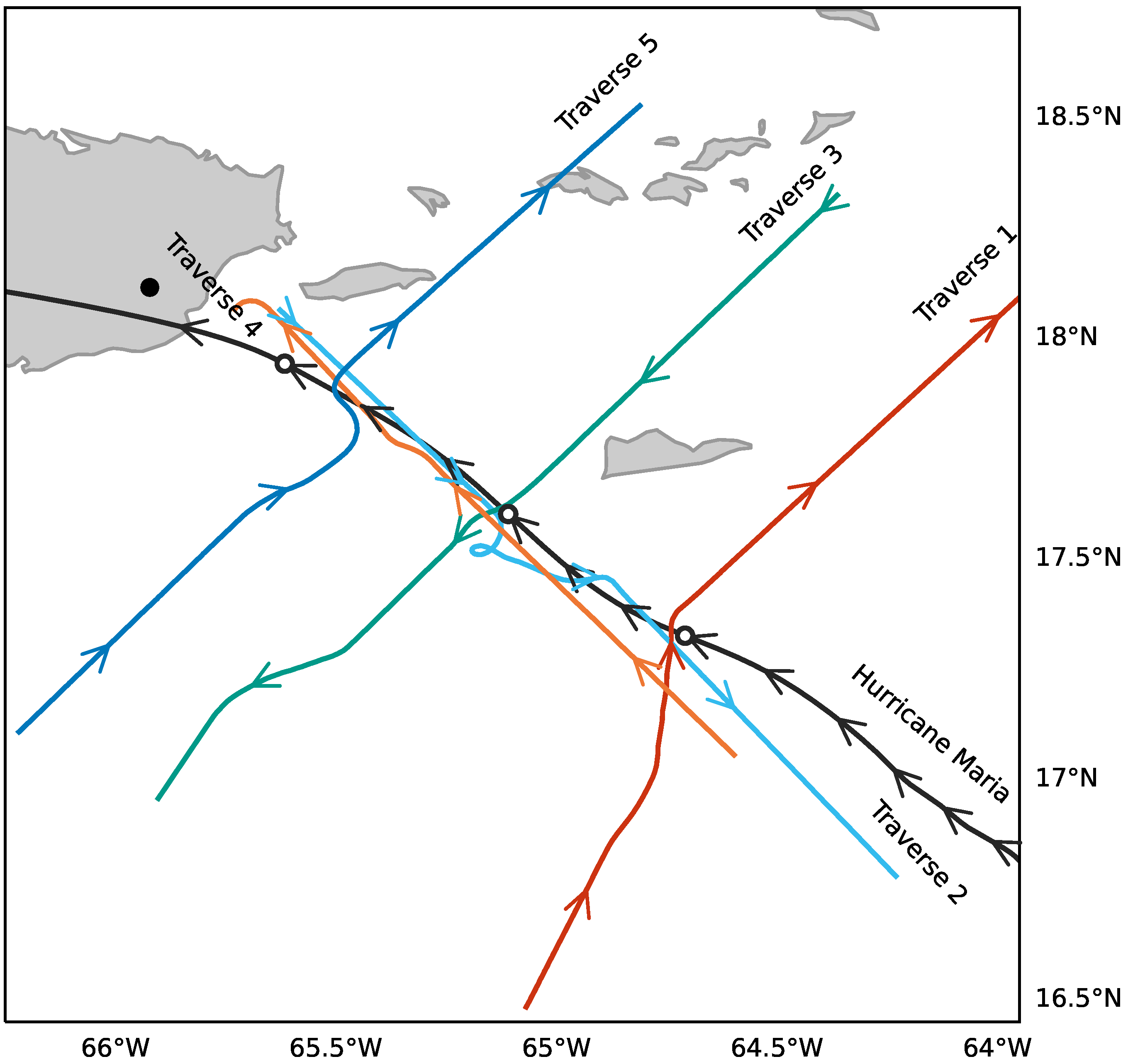
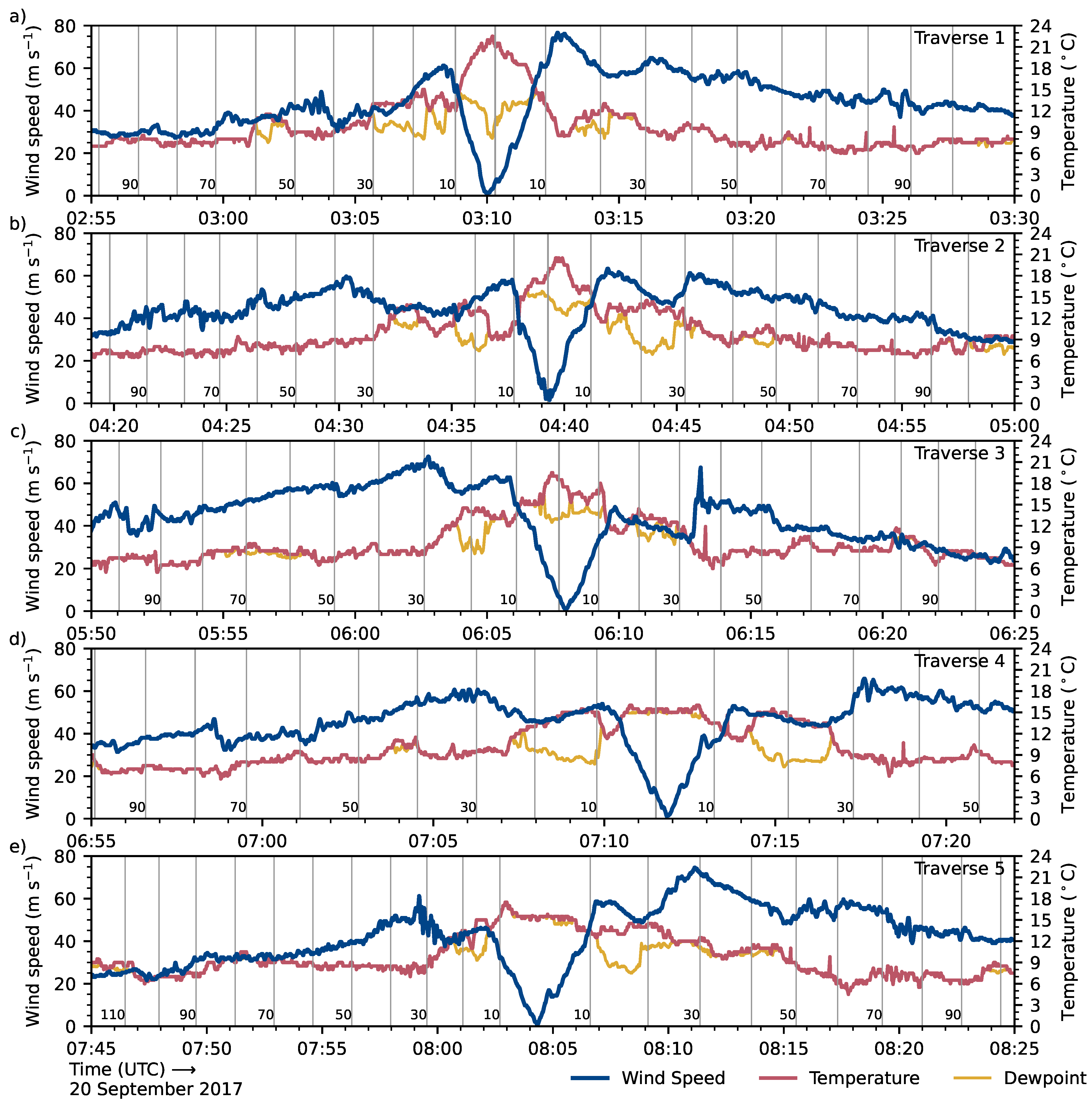
| Traverse | Direction of Traverse | Start (UTC) | End (UTC) |
|---|---|---|---|
| 1 | SW to NE (perpendicular to track) | 2:55 | 3:30 |
| 2 | NW to SE (parallel to track) | 4:20 | 5:00 |
| 3 | NE to SW (perpendicular to track) | 5:50 | 6:25 |
| 4 | SE to NW (parallel to track) | 6:55 | 7:25 |
| 5 | SW to NE (perpendicular to track) | 7:45 | 8:25 |
| Case | |||||||||
|---|---|---|---|---|---|---|---|---|---|
| (m s) | (km) | (km) | (km) | (km) | (m s) | (km) | |||
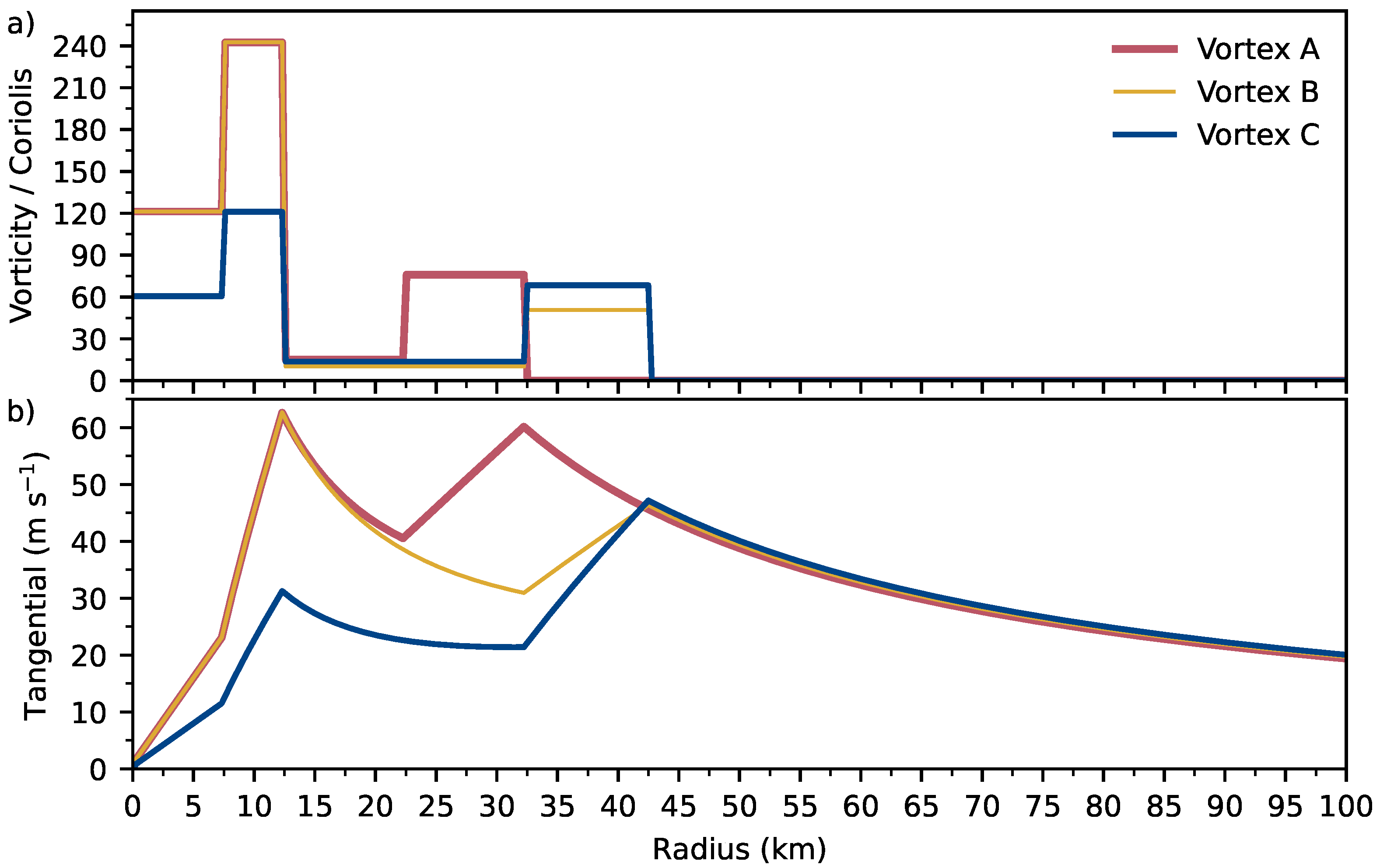
| Vortex A | 60.0 | 7.5 | 12.5 | 22.5 | 32.5 | 20.0 | 100.0 | 0.5 | 0.2 |
| Vortex B | 60.0 | 7.5 | 12.5 | 32.5 | 42.5 | 20.0 | 100.0 | 0.5 | 0.2 |
| Vortex C | 30.0 | 7.5 | 12.5 | 32.5 | 42.5 | 20.0 | 100.0 | 0.5 | 0.2 |
| Vortex | m | |||||
|---|---|---|---|---|---|---|
| (h) | (h) | (%) | (%) | (%) | ||
| A | 2 | 2.79 | 0.36 | 7.79 | 91.82 | 0.39 |
| 4 | 0.94 | 1.07 | 99.67 | 0.33 | 0.00 | |
| B | 4 | 0.44 | 2.28 | 100.00 | 0.00 | 0.00 |
| C | 2 | 0.61 | 1.65 | 6.69 | 84.54 | 8.77 |
| 4 | 0.73 | 1.36 | 99.98 | 0.02 | 0.00 | |
| 6 | 0.84 | 1.20 | 0.00 | 0.00 | 100.00 | |
| 7 | 0.86 | 1.17 | 0.00 | 0.00 | 100.00 |
Disclaimer/Publisher’s Note: The statements, opinions and data contained in all publications are solely those of the individual author(s) and contributor(s) and not of MDPI and/or the editor(s). MDPI and/or the editor(s) disclaim responsibility for any injury to people or property resulting from any ideas, methods, instructions or products referred to in the content. |
© 2023 by the authors. Licensee MDPI, Basel, Switzerland. This article is an open access article distributed under the terms and conditions of the Creative Commons Attribution (CC BY) license (https://creativecommons.org/licenses/by/4.0/).
Share and Cite
Slocum, C.J.; Taft, R.K.; Kossin, J.P.; Schubert, W.H. Barotropic Instability during Eyewall Replacement. Meteorology 2023, 2, 191-221. https://doi.org/10.3390/meteorology2020013
Slocum CJ, Taft RK, Kossin JP, Schubert WH. Barotropic Instability during Eyewall Replacement. Meteorology. 2023; 2(2):191-221. https://doi.org/10.3390/meteorology2020013
Chicago/Turabian StyleSlocum, Christopher J., Richard K. Taft, James P. Kossin, and Wayne H. Schubert. 2023. "Barotropic Instability during Eyewall Replacement" Meteorology 2, no. 2: 191-221. https://doi.org/10.3390/meteorology2020013