A Simple Family of Tropical Cyclone Models

Abstract

This review discusses a simple family of models capable of simulating tropical cyclone life cycles, including intensification, the formation of the axisymmetric version of boundary layer shocks, and the development of an eyewall. Four models are discussed, all of which are axisymmetric, f-plane, three-layer models. All four models have the same parameterizations of convective mass flux and air–sea interaction, but differ in their formulations of the radial and tangential equations of motion, i.e., they have different dry dynamical cores. The most complete model is the primitive equation (PE) model, which uses the unapproximated momentum equations for each of the three layers. The simplest is the gradient balanced (GB) model, which replaces the three radial momentum equations with gradient balance relations and replaces the boundary layer tangential wind equation with a diagnostic equation that is essentially a high Rossby number version of the local Ekman balance. Numerical integrations of the boundary layer equations confirm that the PE model can produce boundary layer shocks, while the GB model cannot. To better understand these differences in GB and PE dynamics, we also consider two hybrid balanced models (HB1 and HB2), which differ from GB only in their treatment of the boundary layer momentum equations. Because their boundary layer dynamics is more accurate than GB, both HB1 and HB2 can produce results more similar to the PE model, if they are solved in an appropriate manner.

1. Introduction

An extensive hierarchy of numerical models allows the tropical cyclone research community to simulate the intensification and movement of tropical cyclones. At the top of this hierarchy, non-hydrostatic, three-dimensional, full-physics models are the ones of most interest for accurate tropical cyclone prediction. At the bottom of this hierarchy, simple, axisymmetric models remain useful for providing a conceptual understanding of certain aspects of the tropical cyclone problem. Here, the purpose is to discuss the equations that comprise a simple family of dynamical models capable of simulating tropical cyclone life cycles, including intensification, the formation of boundary layer shocks, and the development of an eyewall. In particular, we will consider the following four models:

• Primitive Equation Model (PE),
• Hybrid Balanced Model 1 (HB1),
• Hybrid Balanced Model 2 (HB2),
• Gradient Balanced Model (GB).

All four models are axisymmetric and hydrostatic, with only three layers and with moisture predicted only in the lowest layer. All have the same simple parameterizations of convective mass fluxes and air–sea interaction. The most general model considered here is the primitive equation model (PE), which retains the primitive form of the momentum equations in all three layers. It is the only one of the four models that does not filter propagating inertia-gravity waves. The first hybrid balanced model (HB1) assumes gradient balance in the upper two layers but retains the primitive form of the momentum equations in the boundary layer. The second hybrid balanced model (HB2) is slightly simpler than HB1 in that diagnostic forms of the boundary layer momentum equations are used, so that the boundary layer pumping is diagnostic but more accurate than in GB. HB2 is identical to the model briefly studied by Ooyama [1]. Finally, the gradient balanced model (GB) assumes gradient balance in all three layers, with the boundary layer pumping becoming both diagnostic and local. GB is identical to the model extensively studied by Ooyama [2].

This review is organized in the following way. Section 2 and Table 1 give a summary of the three-layer primitive equation model. Then, Section 3 and Section 4, along with Table 2 and Table 3, provide corresponding summaries of the hybrid balanced models HB1 and HB2, while Section 5 and Table 4 give a summary of the fully balanced model GB. Section 6 discusses how the prognostic boundary layer dynamics of the PE and HB1 models can be isolated from the dynamics of the overlying layers and then studied as a one-way interaction problem. The potential vorticity aspects of the four models are then discussed in Section 7.

2. Primitive Equation Model (PE)

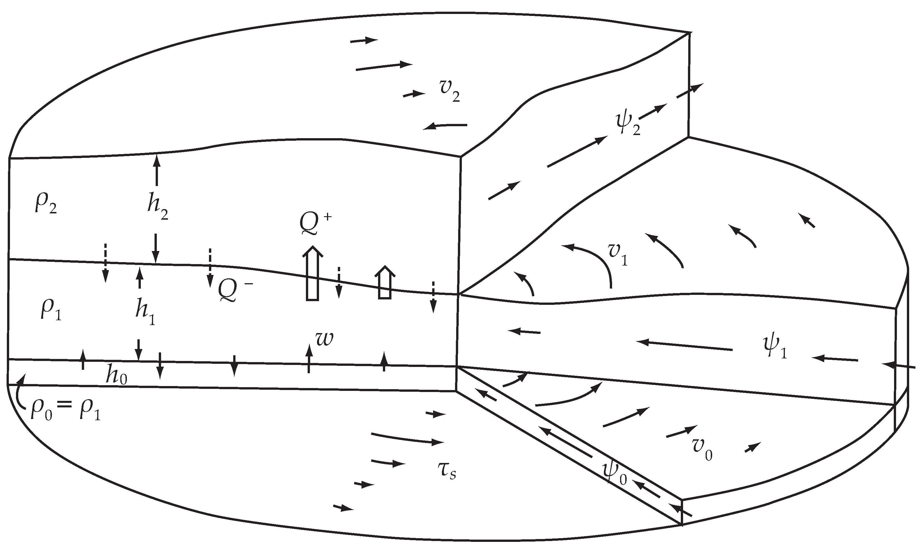
As illustrated in Figure 1, all four models consider axisymmetric motions in three layers of an incompressible fluid on an f-plane with subscripts denoting the layers from 0 for the lowest, 1 for the middle, and 2 for the top layer. The constant density in the lowest two layers is ${\rho }_0={\rho }_1=\rho$, and that in the upper layer is ${\rho }_2=ϵ\rho$, where the constant $ϵ$ satisfies $ϵ<1$. The lowest layer has constant thickness $h_0$, while the upper two layers have variable thicknesses $h_1(r,t)$ and $h_2(r,t)$. The radial velocity components in the three layers are $u_0(r,t)$, $u_1(r,t)$, and $u_2(r,t)$, and the corresponding radial mass fluxes are ${\psi }_0(r,t)=-r{u}_0{h}_0$, ${\psi }_1(r,t)=-r{u}_1{h}_1$, and ${\psi }_2(r,t)=-r{u}_2ϵh_2$. The tangential velocity components in the three layers are $v_0(r,t)$, $v_1(r,t)$, and $v_2(r,t)$.

The hydrostatic pressure at height z, which depends on the weight of the overlying fluid, is given by

$$\begin{array}{cc}\hfill p_1(r,z,t)& =g\rho (h_0+h_1-z)+gϵ\rho h_2,\hfill \\ \hfill p_2(r,z,t)& =gϵ\rho (h_0+h_1+h_2-z),\hfill \end{array}$$

(1)

where the first line applies in layers 0 and 1 (the lower two layers), while the second line applies in layer 2 (the upper layer). Assume that, in the far-field, the upper two layer thicknesses approach the constant values ${\overline{h}}_1$ and ${\overline{h}}_2$, so that the corresponding hydrostatic pressures in the far-field are

$$\begin{array}{cc}\hfill {\overline{p}}_1\left(z\right)& =g\rho (h_0+{\overline{h}}_1-z)+gϵ\rho {\overline{h}}_2,\hfill \\ \hfill {\overline{p}}_2\left(z\right)& =gϵ\rho (h_0+{\overline{h}}_1+{\overline{h}}_2-z).\hfill \end{array}$$

(2)

Defining the geopotential anomalies as ${\varphi }_1=(p_1-{\overline{p}}_1)/\rho$ and ${\varphi }_2=(p_2-{\overline{p}}_2)/ϵ\rho$, it is easily shown from (1) and (2) that

$$\begin{array}{cc}\hfill {\varphi }_1& =g\left\{(h_1-{\overline{h}}_1)+ϵ(h_2-{\overline{h}}_2)\right\},\hfill \\ \hfill {\varphi }_2& =g\left\{(h_1-{\overline{h}}_1)+(h_2-{\overline{h}}_2)\right\},\hfill \end{array}$$

(3)

so that the radial pressure gradient force in the lower two layers is $(1/\rho )(\partial p_1/\partial r)=(\partial {\varphi }_1/\partial r)$, while that in the upper layer is $(1/ϵ\rho )(\partial p_2/\partial r)=(\partial {\varphi }_2/\partial r)$.

The mass continuity equations are

$$\begin{array}{cc}\hfill \frac{\partial \left(r{h}_0{u}_0\right)}{r\partial r}& =-w,\hfill \end{array}$$

(4)

$$\begin{array}{cc}\hfill \frac{\partial h_1}{\partial t}+\frac{\partial \left(r{h}_1{u}_1\right)}{r\partial r}& =w-Q,\hfill \end{array}$$

(5)

$$\begin{array}{cc}\hfill ϵ\frac{\partial h_2}{\partial t}+\frac{\partial \left(rϵh_2{u}_2\right)}{r\partial r}& =Q,\hfill \end{array}$$

(6)

where w is the vertical velocity at the top of the boundary layer and $Q=Q^{+}-Q^{-}$ is the diabatic mass flux between the upper two layers with $Q^{+}$ being the upward diabatic mass flux (heating) from layer 1 to layer 2 and $Q^{-}$ being the downward diabatic mass flux (cooling) from layer 2 to layer 1. Adding the three continuity Equations (4)–(6), noting the cancellation of the terms on the right-hand side, and then integrating over the area and specifying the outer boundary condition to be

$$h_0{u}_0+h_1{u}_1+ϵh_2{u}_2=0\mathrm{at}r=b,$$

(7)

we conclude that

$$\frac{d}{dt}{\int }_0^b\rho (h_0+h_1+ϵh_2)rdr=0,$$

(8)

i.e., the total mass is conserved.

The radial momentum equations for the three layers are given by Equations (1.11)–(1.13) of Table 1, where f is the constant Coriolis parameter, the right-hand side terms are given by

$$\begin{array}{cc}\hfill F_0& =\frac{1}{h_0}\left\{-(w^{-}+\mu )(u_0-u_1)-c_{{}_{\mathrm{D}}}U{u}_0+\frac{\partial {\Lambda }_0^{\left(u\right)}}{r^2\partial r}\right\},\hfill \\ \hfill F_1& =\frac{1}{h_1}\left\{-(w^{+}+\mu )(u_1-u_0)-(Q^{-}+\mu )(u_1-u_2)+\frac{\partial {\Lambda }_1^{\left(u\right)}}{r^2\partial r}\right\},\hfill \\ \hfill F_2& =\frac{1}{ϵh_2}\left\{-(Q^{+}+\mu )(u_2-u_1)+\frac{\partial {\Lambda }_2^{\left(u\right)}}{r^2\partial r}\right\},\hfill \end{array}$$

(9)

$w^{\pm }=\frac{1}{2}\left(\right|w|\pm w)$, so $w=w^{+}-w^{-}$, $\mu$ is the constant coefficient for the frictional stress between the layers, $c_{{}_{\mathrm{D}}}$ is the drag coefficient, $U={\left(u_0^2+v_0^2\right)}^{1/2}$ is the boundary layer wind speed, and the three ${\Lambda }_j^{\left(u\right)}$ terms are horizontal diffusive fluxes for the u-equations as given by (A2) in Appendix A. Similarly, the tangential momentum equations for the three layers are given by Equations (1.14)–(1.16) of Table 1, where the right-hand side terms are given by

$$\begin{array}{cc}\hfill G_0& =\frac{1}{h_0}\left\{-\left(w^{-}+\mu \right)(v_0-v_1)-c_{{}_{\mathrm{D}}}U{v}_0+\frac{\partial {\Lambda }_0^{\left(m\right)}}{r^2\partial r}\right\},\hfill \\ \hfill G_1& =\frac{1}{h_1}\left\{-(w^{+}+\mu )(v_1-v_0)-(Q^{-}+\mu )(v_1-v_2)+\frac{\partial {\Lambda }_1^{\left(m\right)}}{r^2\partial r}\right\},\hfill \\ \hfill G_2& =\frac{1}{ϵh_2}\left\{-(Q^{+}+\mu )(v_2-v_1)+\frac{\partial {\Lambda }_2^{\left(m\right)}}{r^2\partial r}\right\},\hfill \end{array}$$

(10)

where the three ${\Lambda }_j^{\left(m\right)}$ terms are horizontal diffusive fluxes for the m-equations as given by (A4) in Appendix A. Since the momentum Equations (1.11)–(1.16) may have a somewhat unfamiliar form, a derivation from first principles is given in Appendix A.

Rather than predict $h_1(r,t)$ and $h_2(r,t)$ via (5) and (6), it is more convenient to predict ${\varphi }_1(r,t)$ and ${\varphi }_2(r,t)$. The prognostic equations for ${\varphi }_1(r,t)$ and ${\varphi }_2(r,t)$ are easily obtained from (3), (5), and (6), with the result given in Equations (1.17) and (1.18) of Table 1. After ${\varphi }_1(r,t)$ and ${\varphi }_2(r,t)$ are predicted from (1.17) and (1.18), the layer depths can be recovered from (1.1) and (1.2), which follow directly from (3). Note that $\sigma =1-ϵ$ is a measure of static stability.

Now, consider the parameterization of the convective mass flux $Q^{+}$. The equivalent potential temperature budget in the convection is $\eta {\theta }_{ec}={\theta }_{e0}+(\eta -1){\theta }_{e1}$, where $\eta$ is the entrainment parameter, ${\theta }_{ec}$ is the equivalent potential temperature in the convection in the upper layer, ${\theta }_{e0}$ is the equivalent potential temperature in the boundary layer, and ${\theta }_{e1}$ is the equivalent potential temperature in layer 1. We assume that the convection has neutral buoyancy in the upper layer, so that ${\theta }_{ec}={\theta }_{e2}^{\ast }$, where ${\theta }_{e2}^{\ast }$ is the saturation equivalent potential temperature in the upper layer. Combining these last two relations, we obtain Equation (1.9) of Table 1. Note that conditional instability occurs in a column when ${\theta }_{e0}>{\theta }_{e2}^{\ast }$, which means $\eta >1$ since ${\theta }_{e2}^{\ast }>{\theta }_{e1}$. The equivalent potential temperature of the middle layer is assumed to be a specified parameter, while the boundary layer equivalent potential temperature, ${\theta }_{e0}$ (a prognostic variable), and the upper layer saturation equivalent potential temperature, ${\theta }_{e2}^{\ast }$ (a diagnostic variable), depend on radius and time. Finally, $Q^{+}$ is given by $Q^{+}=\eta w^{+}$, so it then follows that $Q=\eta w^{+}-Q^{-}$ as indicated by Equation (1.10) of Table 1, where $Q^{-}$ is a specified parameter (typically zero).

Table 1. Summary of the PE model. The upper half of the table lists the diagnostic equations, while the lower half lists the nine prognostic equations. The right-hand sides of (1.11)–(1.16) are defined in (9) and (10). Because the radial components $u_1(r,t)$ and $u_2(r,t)$ are predicted, the PE model allows propagating inertia-gravity waves. Because the boundary layer radial and tangential components $u_0(r,t)$ and $v_0(r,t)$ are predicted, and because large inflow often occurs in the boundary layer, the PE model can develop boundary layer shocks. The diabatic mass flux $Q^{+}$ depends on boundary layer convergence ($w>0$) and the entrainment parameter $\eta$, which in turn depends on the boundary layer equivalent potential temperature ${\theta }_{e0}$, predicted by (1.19), and the upper tropospheric saturation equivalent potential temperature ${\theta }_{e2}^{\ast }$, diagnosed from (1.4).

Primitive Equation Model (PE)
Diagnostic Equations:
Layer thicknesses:			Saturation equivalent potential temperatures:
	${\displaystyle h_1={\overline{h}}_1+\frac{1}{g\sigma }({\varphi }_1-ϵ{\varphi }_2)}$	(1.1)		${\displaystyle {\theta }_{es}^{\ast }={\overline{\theta }}_{es}^{\ast }-\frac{2.0}{c_p}{\varphi }_1}$	(1.3)
	${\displaystyle h_2={\overline{h}}_2+\frac{1}{g\sigma }({\varphi }_2-{\varphi }_1)}$	(1.2)		${\displaystyle {\theta }_{e2}^{\ast }={\overline{\theta }}_{e2}^{\ast }+\frac{10.3}{c_p}({\varphi }_2-{\varphi }_1)}$	(1.4)
Air-sea interaction:			Ekman pumping:
	${\displaystyle U={\left(u_0^2+v_0^2\right)}^{1/2}}$	(1.5)		${\displaystyle w=-h_0\frac{\partial \left(r{u}_0\right)}{r\partial r}}$	(1.7)
	${\displaystyle c_{{}_{\mathrm{E}}}=c_{{}_{\mathrm{D}}}=(0.5+0.06U)·{10}^{-3}}$	(1.6)		${\displaystyle w^{\pm }=\frac{1}{2}\left(\left|w\right|\pm w\right)}$	(1.8)
Diabatic mass flux:
	${\displaystyle \eta =1+\frac{{\theta }_{e0}-{\theta }_{e2}^{\ast }}{{\theta }_{e2}^{\ast }-{\theta }_{e1}}}$	(1.9)		${\displaystyle Q=Q^{+}-Q^{-}}$    with    ${\displaystyle Q^{+}=\eta w^{+}}$	(1.10)
Prognostic Equations:
Radial wind components:
	${\displaystyle \frac{\partial u_0}{\partial t}+u_0\frac{\partial u_0}{\partial r}-\left(f+\frac{v_0}{r}\right)v_0+\frac{\partial {\varphi }_1}{\partial r}=F_0}$				(1.11)
	${\displaystyle \frac{\partial u_1}{\partial t}+u_1\frac{\partial u_1}{\partial r}-\left(f+\frac{v_1}{r}\right)v_1+\frac{\partial {\varphi }_1}{\partial r}=F_1}$				(1.12)
	${\displaystyle \frac{\partial u_2}{\partial t}+u_2\frac{\partial u_2}{\partial r}-\left(f+\frac{v_2}{r}\right)v_2+\frac{\partial {\varphi }_2}{\partial r}=F_2}$				(1.13)
Tangential wind components:
	${\displaystyle \frac{\partial v_0}{\partial t}+u_0\frac{\partial v_0}{\partial r}+\left(f+\frac{v_0}{r}\right)u_0=G_0}$				(1.14)
	${\displaystyle \frac{\partial v_1}{\partial t}+u_1\frac{\partial v_1}{\partial r}+\left(f+\frac{v_1}{r}\right)u_1=G_1}$				(1.15)
	${\displaystyle \frac{\partial v_2}{\partial t}+u_2\frac{\partial v_2}{\partial r}+\left(f+\frac{v_2}{r}\right)u_2=G_2}$				(1.16)
Geopotential anomalies:
	${\displaystyle \frac{\partial {\varphi }_1}{\partial t}+g\frac{\partial \left[r(u_1{h}_1+u_2ϵh_2)\right]}{r\partial r}=gw}$				(1.17)
	${\displaystyle \frac{\partial {\varphi }_2}{\partial t}+g\frac{\partial \left[r(u_1{h}_1+u_2{h}_2)\right]}{r\partial r}=g\left(w+\frac{\sigma }{ϵ}Q\right)}$				(1.18)
Boundary layer equivalent potential temperature:
	${\displaystyle \frac{\partial {\theta }_{e0}}{\partial t}+u_0\frac{\partial {\theta }_{e0}}{\partial r}+\frac{w^{-}}{h_0}({\theta }_{e0}-{\theta }_{e1})=\frac{c_{{}_{\mathrm{E}}}U}{h_0}({\theta }_{es}^{\ast }-{\theta }_{e0})}$				(1.19)

Table 1. Summary of the PE model. The upper half of the table lists the diagnostic equations, while the lower half lists the nine prognostic equations. The right-hand sides of (1.11)–(1.16) are defined in (9) and (10). Because the radial components $u_1(r,t)$ and $u_2(r,t)$ are predicted, the PE model allows propagating inertia-gravity waves. Because the boundary layer radial and tangential components $u_0(r,t)$ and $v_0(r,t)$ are predicted, and because large inflow often occurs in the boundary layer, the PE model can develop boundary layer shocks. The diabatic mass flux $Q^{+}$ depends on boundary layer convergence ($w>0$) and the entrainment parameter $\eta$, which in turn depends on the boundary layer equivalent potential temperature ${\theta }_{e0}$, predicted by (1.19), and the upper tropospheric saturation equivalent potential temperature ${\theta }_{e2}^{\ast }$, diagnosed from (1.4).

Primitive Equation Model (PE)
Diagnostic Equations:
Layer thicknesses:			Saturation equivalent potential temperatures:
	${\displaystyle h_1={\overline{h}}_1+\frac{1}{g\sigma }({\varphi }_1-ϵ{\varphi }_2)}$	(1.1)		${\displaystyle {\theta }_{es}^{\ast }={\overline{\theta }}_{es}^{\ast }-\frac{2.0}{c_p}{\varphi }_1}$	(1.3)
	${\displaystyle h_2={\overline{h}}_2+\frac{1}{g\sigma }({\varphi }_2-{\varphi }_1)}$	(1.2)		${\displaystyle {\theta }_{e2}^{\ast }={\overline{\theta }}_{e2}^{\ast }+\frac{10.3}{c_p}({\varphi }_2-{\varphi }_1)}$	(1.4)
Air-sea interaction:			Ekman pumping:
	${\displaystyle U={\left(u_0^2+v_0^2\right)}^{1/2}}$	(1.5)		${\displaystyle w=-h_0\frac{\partial \left(r{u}_0\right)}{r\partial r}}$	(1.7)
	${\displaystyle c_{{}_{\mathrm{E}}}=c_{{}_{\mathrm{D}}}=(0.5+0.06U)·{10}^{-3}}$	(1.6)		${\displaystyle w^{\pm }=\frac{1}{2}\left(\left|w\right|\pm w\right)}$	(1.8)
Diabatic mass flux:
	${\displaystyle \eta =1+\frac{{\theta }_{e0}-{\theta }_{e2}^{\ast }}{{\theta }_{e2}^{\ast }-{\theta }_{e1}}}$	(1.9)		${\displaystyle Q=Q^{+}-Q^{-}}$    with    ${\displaystyle Q^{+}=\eta w^{+}}$	(1.10)
Prognostic Equations:
Radial wind components:
	${\displaystyle \frac{\partial u_0}{\partial t}+u_0\frac{\partial u_0}{\partial r}-\left(f+\frac{v_0}{r}\right)v_0+\frac{\partial {\varphi }_1}{\partial r}=F_0}$				(1.11)
	${\displaystyle \frac{\partial u_1}{\partial t}+u_1\frac{\partial u_1}{\partial r}-\left(f+\frac{v_1}{r}\right)v_1+\frac{\partial {\varphi }_1}{\partial r}=F_1}$				(1.12)
	${\displaystyle \frac{\partial u_2}{\partial t}+u_2\frac{\partial u_2}{\partial r}-\left(f+\frac{v_2}{r}\right)v_2+\frac{\partial {\varphi }_2}{\partial r}=F_2}$				(1.13)
Tangential wind components:
	${\displaystyle \frac{\partial v_0}{\partial t}+u_0\frac{\partial v_0}{\partial r}+\left(f+\frac{v_0}{r}\right)u_0=G_0}$				(1.14)
	${\displaystyle \frac{\partial v_1}{\partial t}+u_1\frac{\partial v_1}{\partial r}+\left(f+\frac{v_1}{r}\right)u_1=G_1}$				(1.15)
	${\displaystyle \frac{\partial v_2}{\partial t}+u_2\frac{\partial v_2}{\partial r}+\left(f+\frac{v_2}{r}\right)u_2=G_2}$				(1.16)
Geopotential anomalies:
	${\displaystyle \frac{\partial {\varphi }_1}{\partial t}+g\frac{\partial \left[r(u_1{h}_1+u_2ϵh_2)\right]}{r\partial r}=gw}$				(1.17)
	${\displaystyle \frac{\partial {\varphi }_2}{\partial t}+g\frac{\partial \left[r(u_1{h}_1+u_2{h}_2)\right]}{r\partial r}=g\left(w+\frac{\sigma }{ϵ}Q\right)}$				(1.18)
Boundary layer equivalent potential temperature:
	${\displaystyle \frac{\partial {\theta }_{e0}}{\partial t}+u_0\frac{\partial {\theta }_{e0}}{\partial r}+\frac{w^{-}}{h_0}({\theta }_{e0}-{\theta }_{e1})=\frac{c_{{}_{\mathrm{E}}}U}{h_0}({\theta }_{es}^{\ast }-{\theta }_{e0})}$				(1.19)

To include the effects of the warm core on convection, we need to interpret ${\theta }_{e2}^{\ast }$ in terms of potential temperature, even though potential temperature does not appear explicitly in the three-layer model. This can be accomplished by writing the hydrostatic equation for a compressible fluid in the differential form $d(\varphi -\overline{\varphi })=-c_p(\theta -\overline{\theta })d{(p/p_{00})}^{\kappa }$, where $\varphi -\overline{\varphi }$ is the deviation of the geopotential $\varphi$ from its far-field value $\overline{\varphi }$, $\theta -\overline{\theta }$ is the deviation of the potential temperature $\theta$ from its far-field value $\overline{\theta }$, $p_{00}=1000$ hPa is the reference pressure, and $\kappa =R/c_p$. Based on a discrete form of this hydrostatic equation, it is reasonable to define the middle-tropospheric potential temperature anomaly ${\theta }_m-{\overline{\theta }}_m$, where ${\overline{\theta }}_m$ is the middle-tropospheric potential temperature in the far field, as

$$c_p\left({\theta }_m-{\overline{\theta }}_m\right)=\frac{{\varphi }_2-{\varphi }_1}{{\left(0.7\right)}^{\kappa }-{\left(0.3\right)}^{\kappa }}=5.15({\varphi }_2-{\varphi }_1),$$

(11)

where we use 700 and 300 hPa as representative values of the pressure in the upper two layers. Thus, in the context of the three-layer model, ${\varphi }_2-{\varphi }_1$ can be interpreted as proportional to the middle-tropospheric potential temperature anomaly. Using a Taylor series approximation (or simple inspection of the upper tropospheric spacing of $\theta$-lines and ${\theta }_e^{\ast }$-lines on a thermodynamic diagram), we can justify the approximation ${\theta }_{e2}^{\ast }={\overline{\theta }}_{e2}^{\ast }+2.0({\theta }_m-{\overline{\theta }}_m)$, where ${\overline{\theta }}_{e2}^{\ast }$ is the upper layer saturation equivalent potential temperature in the far field. Combining this approximation with (11) yields Equation (1.4) of Table 1. The spatial and temporal dependence of ${\theta }_{e2}^{\ast }$ can serve as an important negative feedback on tropical cyclone intensification, since an evolving warm core can reduce ${\theta }_{e0}-{\theta }_{e2}^{\ast }$ and hence reduce $\eta$ via Equation (1.9).

The equivalent potential temperature is predicted only in the lowest layer. In flux form, the boundary layer equivalent potential temperature equation is

$$\frac{\partial \left(h_0{\theta }_{e0}\right)}{\partial t}+\frac{\partial \left(r{h}_0{u}_0{\theta }_{e0}\right)}{r\partial r}+w^{+}{\theta }_{e0}-w^{-}{\theta }_{e1}=c_{{}_{\mathrm{E}}}U\left({\theta }_{es}^{\ast }-{\theta }_{e0}\right),$$

(12)

where $c_{{}_{\mathrm{E}}}$ is the exchange coefficient, $U={(u_0^2+v_0^2)}^{1/2}$ is the boundary layer wind speed, and ${\theta }_{es}^{\ast }$ is the saturation equivalent potential temperature at the sea-surface temperature and pressure. When (12) is converted to advective form, we obtain Equation (1.19) of Table 1. Important controls on moist convection occur in the terms of (1.19). In the tropical cyclone inner region, where there is boundary layer pumping ($w>0$ so that $w^{-}=0$), the term $w^{-}({\theta }_{e0}-{\theta }_{e1})/h_0$ vanishes. However, in the tropical cyclone outer region, where there is boundary layer suction ($w<0$ so that $w^{-}>0$), the term $w^{-}({\theta }_{e0}-{\theta }_{e1})/h_0$ is positive and tends to produce a decrease of boundary layer equivalent potential temperature through the downward transport of dry middle-tropospheric air (${\theta }_{e1}<{\theta }_{e0}$). Air–sea interaction plays a crucial role in maintaining high values of ${\theta }_{e0}$ through the surface flux term $c_{{}_{\mathrm{E}}}U({\theta }_{es}^{\ast }-{\theta }_{e0})/h_0$. The factor $c_{{}_{\mathrm{E}}}U$ becomes large in regions of high surface winds, while the saturation equivalent potential temperature at the sea surface (${\theta }_{es}^{\ast }$) becomes large in regions where the surface pressure is low, an effect that is incorporated through Equation (1.3) of Table 1. Both effects enhance the surface flux $c_{{}_{\mathrm{E}}}U({\theta }_{es}^{\ast }-{\theta }_{e0})$ and can maintain ${\theta }_{e0}>{\theta }_{e2}^{\ast }$, and hence $\eta$ slightly larger than unity, even though an upper tropospheric warm core is being produced and ${\theta }_{e2}^{\ast }$ is increasing through Equation (1.4).

Since ${\theta }_{es}^{\ast }$ depends on both the sea surface temperature and pressure, and since the sea surface pressure depends on ${\varphi }_1$, we should regard ${\theta }_{es}^{\ast }$ as a dependent variable that increases as the sea surface pressure decreases. Using a Taylor series approximation (or simple inspection of the lower tropospheric spacing of p-lines and ${\theta }_e^{\ast }$-lines on a thermodynamic diagram) the dependent variable ${\theta }_{es}^{\ast }$ can be parameterized as given in Equation (1.3) of Table 1. Thus, in the far field, where the geopotential anomaly ${\varphi }_1$ is very small, the value of ${\theta }_{es}^{\ast }$ is ${\overline{\theta }}_{es}^{\ast }=372\mathrm{K}$ for the typical case examined in Section 8. However, if ${\varphi }_1$ in the inner core is approximately $-5000$ m${}^2$ s${}^{-2}$ (i.e., a $-50$ hPa sea surface pressure anomaly), then the value of ${\theta }_{es}^{\ast }$ is locally increased to $382\mathrm{K}$. This dependence of ${\theta }_{es}^{\ast }$ on ${\varphi }_1$ plays an important role in enhancing the surface flux of ${\theta }_e$ in the inner core of the vortex. Finally, we list in Equation (1.6) the assumed $c_{{}_{\mathrm{D}}}$ and $c_{{}_{\mathrm{E}}}$ formulas used by Ooyama for his standard case. The results of some very interesting experiments with other parameterizations for $c_{{}_{\mathrm{D}}}$ and $c_{{}_{\mathrm{E}}}$ are discussed by Ooyama ([2], Section 14).

The nine prognostic variables of the primitive equation model are $u_0(r,t)$, $u_1(r,t)$, $u_2(r,t)$, $v_0(r,t)$, $v_1(r,t)$, $v_2(r,t)$, ${\varphi }_1(r,t)$, ${\varphi }_2(r,t)$, and ${\theta }_{e0}(r,t)$, so all the other variables are diagnostic. The steps of the numerical integration procedure start with knowledge of these nine prognostic variables, either from the initial conditions or from the previous time step. The procedure for advancing one time level is as follows:

1.

Specify desired values for the various fixed parameters: g, $c_p$, f, $ϵ$ or $\sigma =1-ϵ$, $h_0$, ${\overline{h}}_1$, ${\overline{h}}_2$, ${\overline{\theta }}_{es}^{\ast }$, ${\overline{\theta }}_{e2}^{\ast }$, ${\theta }_{e1}$, $Q^{-}$, $\mu$, and K, where K is the constant kinematic coefficient of eddy viscosity appearing in the equations for the horizontal diffusive fluxes given in (A2) and (A4) in Appendix A.

2.

Using the known geopotential anomalies ${\varphi }_1(r,t)$ and ${\varphi }_2(r,t)$, diagnose the layer depths $h_1(r,t)$ and $h_2(r,t)$ from (1.1) and (1.2), the sea-surface saturation equivalent potential temperature ${\theta }_{es}^{\ast }(r,t)$ from (1.3), and the upper tropospheric saturation equivalent potential temperature ${\theta }_{e2}^{\ast }(r,t)$ from (1.4).

3.

Compute the boundary layer wind speed $U(r,t)$ from (1.5), and then the exchange coefficient $c_{{}_{\mathrm{E}}}(r,t)$ and the drag coefficient $c_{{}_{\mathrm{D}}}(r,t)$ from (1.6).

4.

Using (1.7), diagnose the boundary layer vertical velocity $w(r,t)$ from the known boundary layer radial velocity $u_0(r,t)$, then compute $w^{+}(r,t)$ and $w^{-}(r,t)$ from (1.8).

5.

Using the constant ${\theta }_{e1}$, the diagnosed ${\theta }_{e2}^{\ast }(r,t)$, and the known ${\theta }_{e0}(r,t)$, diagnose the entrainment parameter $\eta (r,t)$ from (1.9); then, compute the diabatic mass flux $Q(r,t)$ from (1.10).

6.

Using the definitions of $F_j(r,t)$ and $G_j(r,t)$ given in (9) and (10), predict new values of the radial and tangential wind components from (1.11)–(1.16).

7.

Using the known radial velocity components $u_1(r,t)$ and $u_2(r,t)$, predict the geopotential anomalies ${\varphi }_1(r,t)$ and ${\varphi }_2(r,t)$ via (1.17) and (1.18).

8.

Using the known boundary layer radial velocity $u_0(r,t)$, the diagnosed boundary layer suction $w^{-}(r,t)$, and the diagnosed ${\theta }_{es}^{\ast }(r,t)$, predict the boundary layer equivalent potential temperature ${\theta }_{e0}(r,t)$ via (1.19), and then return to step 2 for the beginning of the next time step.

The dynamical core of this model has no explicit thermodynamics. Since there is a discontinuity in the density at the interface between layers 1 and 2, we can regard this interface as containing many constant-density surfaces packed closely together. Through the analogy between density surfaces and potential temperature surfaces (see [3]), we can also regard this interface as containing many closely packed $\theta$ surfaces. The mass flux $Q^{+}$ can therefore be regarded as being due to latent heat release in the moist convective updrafts that carry cloudy air across $\theta$ surfaces into the upper troposphere. The four models discussed here connect $Q^{+}$ to boundary layer convergence, boundary layer ${\theta }_e$, and upper tropospheric temperature in a very simple way. It should be noted that non-hydrostatic, full-physics models of tropical cyclones explicitly model the details of water and ice microphysics, the different categories of ice, the different fall velocities of liquid and ice, the role of aerosols in the size distributions of condensate, etc. The simplified three-layer models presented here neglect all such microphysical details, but do capture the most fundamental effect of precipitating moist convection, i.e., the convective mass flux across $\theta$ surfaces from the lower troposphere to the upper troposphere. The dynamical adjustments to this mass flux are what produce the lower tropospheric cyclone and the upper tropospheric anticyclone.

Equations (1.1)–(1.19) constitute one of the simplest PE models capable of simulating tropical cyclone life cycles, including intensification, the formation of boundary layer shocks, and the development of an eyewall.

3. Hybrid Balanced Model 1 (HB1)

The equations for the HB1 model are listed in Table 2. The most obvious difference between Table 1 and Table 2 is that for HB1 the number of diagnostic equations has increased from ten to fourteen, while the number of prognostic equations has decreased from nine to five. The ten diagnostic equations in Table 1 carry over directly to Table 2, and four additional diagnostic equations appear. In the HB1 model, the prognostic equations for $u_1$ and $u_2$ are discarded and replaced by the gradient wind relations (2.11) and (2.12). With gradient balance in the middle and upper layers, the predictions of $v_1$ and $v_2$ are redundant with the predictions of ${\varphi }_1$ and ${\varphi }_2$. In other words, taking the local time derivative of the gradient wind equation yields

$$\left(f+\frac{2v_j}{r}\right)\frac{\partial v_j}{\partial t}=\frac{\partial }{\partial r}\left(\frac{\partial {\varphi }_j}{\partial t}\right)\mathrm{for}j=1,2.$$

(13)

Using the tangential wind equation to eliminate $(\partial v_j/\partial t)$ and the mass continuity principle to eliminate $(\partial {\varphi }_j/\partial t)$, we obtain the diagnostic Equations (2.13) and (2.14) of Table 2, where the local inertial stability $S_j$ in layer j is defined by

$$S_j=\left(f+\frac{2v_j}{r}\right)\left(\frac{f+{\zeta }_j}{g{h}_j}\right)=\left(f+\frac{2v_j}{r}\right)\frac{P_j}{g{\overline{h}}_j}\mathrm{for}j=1,2$$

(14)

where ${\zeta }_j=\partial \left(r{v}_j\right)/r\partial r$ is the relative vorticity in layer j and $P_j=(f+{\zeta }_j){\overline{h}}_j/h_j$ is the potential vorticity in layer j. Equations (2.13) and (2.14) constitute a coupled pair of second order diagnostic equations (i.e., the Eliassen transverse circulation equations given in reference [4]) for the radial mass fluxes ${\psi }_1=-r{u}_1{h}_1$ and ${\psi }_2=-r{u}_2ϵh_2$. These radial mass fluxes are forced by the diabatic and frictional effects that appear on the right-hand sides of (2.13) and (2.14), while the spatial distribution of these fluxes is shaped by the inertial stability factors on the left-hand sides. Since (2.13) and (2.14) are diagnostic equations, an instantaneous change in the diabatic and frictional forcing produces an immediate response in the entire fluid. This “action at a distance” property does not occur in the PE model since fluctuations of the inner core forcing excite inertia-gravity waves, which require a finite time to spread information laterally and thereby adjust the radial mass fluxes in the surrounding fluid. The forcing terms on the right-hand side of the transverse circulation Equations (2.13) and (2.14) involve $G_1$, $G_2$, $(\partial w/\partial r)$, and $(\partial Q/\partial r)$. For the idealized situation in which the absolute angular momentum is materially conserved in the upper two layers, we have $G_1=G_2=0$, so the forcing of the transverse circulation then involves only the radial derivatives of the boundary layer pumping w and the diabatic mass flux Q. If the diabatic mass flux Q were to vanish and w were to be largest at the center of the vortex, then $(\partial w/\partial r)<0$ over a core region, which results in $u_1>0$ and $u_2>0$, with the relative magnitudes of $u_1$ and $u_2$ determined by the relative magnitudes of the inertial stability factors $S_1$ and $S_2$. Such radial outflow leads to the spin-down (at all radii) of the cyclonic vortex in layers 1 and 2. As discussed by Greenspan and Howard [5] and Greenspan ([6], Sections 2.3 and 2.4), this is what occurs in a laminar Ekman layer with a no-slip lower boundary condition. However, as discussed by Eliassen and Lystad [7], the situation is different in a turbulent Ekman layer with a thin Prandtl surface layer and stress condition at the lower boundary. In that case, the Ekman pumping does not maximize at the vortex axis, but rather at some finite radius. This effect seems crucial in understanding the structure of the eye and eyewall. All four models discussed here can simulate this important effect.

Table 2. Summary of the HB1 model. The upper half of the table lists the diagnostic equations, while the lower half lists the five prognostic equations. As indicated in (2.11) and (2.12), gradient balance is assumed in the upper two layers, but, as indicated in (2.15) and (2.16), the primitive forms of the momentum equations are retained in the boundary layer, thus allowing the formation of boundary layer shocks. Because the prognostic equations for $u_1(r,t)$ and $u_2(r,t)$ have been discarded and replaced by the coupled Eliassen Equations (2.13) and (2.14), propagating inertia-gravity waves are filtered in the HB1 model. A sufficient (but not necessary) condition for the uniqueness of the solutions ${\psi }_1,{\psi }_2$ of the Eliassen equations is that $S_1\ge 0$ and $S_2\ge 0$. Numerical integrations of the Eliassen equations reveal that $S_2$ can become negative at some distance from the cyclone center, but no difficulty is encountered in the solution of the discretized Eliassen equations if a direct method of solution (such as Gaussian elimination) is used.

Hybrid Balanced Model 1 (HB1)
Diagnostic Equations:
Layer thicknesses:			Saturation equivalent potential temperatures:
	${\displaystyle h_1={\overline{h}}_1+\frac{1}{g\sigma }({\varphi }_1-ϵ{\varphi }_2)}$	(2.1)		${\displaystyle {\theta }_{es}^{\ast }={\overline{\theta }}_{es}^{\ast }-\frac{2.0}{c_p}{\varphi }_1}$	(2.3)
	${\displaystyle h_2={\overline{h}}_2+\frac{1}{g\sigma }({\varphi }_2-{\varphi }_1)}$	(2.2)		${\displaystyle {\theta }_{e2}^{\ast }={\overline{\theta }}_{e2}^{\ast }+\frac{10.3}{c_p}({\varphi }_2-{\varphi }_1)}$	(2.4)
Air-sea interaction:			Ekman pumping:
	${\displaystyle U={\left(u_0^2+v_0^2\right)}^{1/2}}$	(2.5)		${\displaystyle w=-h_0\frac{\partial \left(r{u}_0\right)}{r\partial r}}$	(2.7)
	${\displaystyle c_{{}_{\mathrm{E}}}=c_{{}_{\mathrm{D}}}=(0.5+0.06U)·{10}^{-3}}$	(2.6)		${\displaystyle w^{\pm }=\frac{1}{2}\left(\left|w\right|\pm w\right)}$	(2.8)
Diabatic mass flux:			Gradient balance equations:
	${\displaystyle \eta =1+\frac{{\theta }_{e0}-{\theta }_{e2}^{\ast }}{{\theta }_{e2}^{\ast }-{\theta }_{e1}}}$	(2.9)		${\displaystyle \left(f+\frac{v_1}{r}\right)v_1=\frac{\partial {\varphi }_1}{\partial r}}$	(2.11)
	${\displaystyle Q=Q^{+}-Q^{-}}$    with    ${\displaystyle Q^{+}=\eta w^{+}}$	(2.10)		${\displaystyle \left(f+\frac{v_2}{r}\right)v_2=\frac{\partial {\varphi }_2}{\partial r}}$	(2.12)
Transverse circulation: (where ${\psi }_1=-r{u}_1{h}_1$ and ${\psi }_2=-r{u}_2ϵh_2$)
	${\displaystyle r\frac{\partial }{\partial r}\left(\frac{\partial ({\psi }_1+{\psi }_2)}{r\partial r}\right)-S_1{\psi }_1=\frac{1}{g}\left(f+\frac{2v_1}{r}\right)r{G}_1-r\frac{\partial w}{\partial r}}$				(2.13)
	${\displaystyle r\frac{\partial }{\partial r}\left(\frac{\partial ({\psi }_1+{ϵ}^{-1}{\psi }_2)}{r\partial r}\right)-S_2{ϵ}^{-1}{\psi }_2=\frac{1}{g}\left(f+\frac{2v_2}{r}\right)r{G}_2-r\frac{\partial }{\partial r}\left(w+\frac{\sigma }{ϵ}Q\right)}$				(2.14)
Prognostic Equations:
Boundary layer radial and tangential wind components:
	${\displaystyle \frac{\partial u_0}{\partial t}+u_0\frac{\partial u_0}{\partial r}-\left(f+\frac{v_0}{r}\right)v_0+\frac{\partial {\varphi }_1}{\partial r}=F_0}$				(2.15)
	${\displaystyle \frac{\partial v_0}{\partial t}+u_0\frac{\partial v_0}{\partial r}+\left(f+\frac{v_0}{r}\right)u_0=G_0}$				(2.16)
Geopotential anomalies:
	${\displaystyle \frac{\partial {\varphi }_1}{\partial t}=g\frac{\partial ({\psi }_1+{\psi }_2)}{r\partial r}+gw}$				(2.17)
	${\displaystyle \frac{\partial {\varphi }_2}{\partial t}=g\frac{\partial ({\psi }_1+{ϵ}^{-1}{\psi }_2)}{r\partial r}+g\left(w+\frac{\sigma }{ϵ}Q\right)}$				(2.18)
Boundary layer equivalent potential temperature:
	${\displaystyle \frac{\partial {\theta }_{e0}}{\partial t}+u_0\frac{\partial {\theta }_{e0}}{\partial r}+\frac{w^{-}}{h_0}({\theta }_{e0}-{\theta }_{e1})=\frac{c_{{}_{\mathrm{E}}}U}{h_0}({\theta }_{es}^{\ast }-{\theta }_{e0})}$				(2.19)

Table 2. Summary of the HB1 model. The upper half of the table lists the diagnostic equations, while the lower half lists the five prognostic equations. As indicated in (2.11) and (2.12), gradient balance is assumed in the upper two layers, but, as indicated in (2.15) and (2.16), the primitive forms of the momentum equations are retained in the boundary layer, thus allowing the formation of boundary layer shocks. Because the prognostic equations for $u_1(r,t)$ and $u_2(r,t)$ have been discarded and replaced by the coupled Eliassen Equations (2.13) and (2.14), propagating inertia-gravity waves are filtered in the HB1 model. A sufficient (but not necessary) condition for the uniqueness of the solutions ${\psi }_1,{\psi }_2$ of the Eliassen equations is that $S_1\ge 0$ and $S_2\ge 0$. Numerical integrations of the Eliassen equations reveal that $S_2$ can become negative at some distance from the cyclone center, but no difficulty is encountered in the solution of the discretized Eliassen equations if a direct method of solution (such as Gaussian elimination) is used.

Hybrid Balanced Model 1 (HB1)
Diagnostic Equations:
Layer thicknesses:			Saturation equivalent potential temperatures:
	${\displaystyle h_1={\overline{h}}_1+\frac{1}{g\sigma }({\varphi }_1-ϵ{\varphi }_2)}$	(2.1)		${\displaystyle {\theta }_{es}^{\ast }={\overline{\theta }}_{es}^{\ast }-\frac{2.0}{c_p}{\varphi }_1}$	(2.3)
	${\displaystyle h_2={\overline{h}}_2+\frac{1}{g\sigma }({\varphi }_2-{\varphi }_1)}$	(2.2)		${\displaystyle {\theta }_{e2}^{\ast }={\overline{\theta }}_{e2}^{\ast }+\frac{10.3}{c_p}({\varphi }_2-{\varphi }_1)}$	(2.4)
Air-sea interaction:			Ekman pumping:
	${\displaystyle U={\left(u_0^2+v_0^2\right)}^{1/2}}$	(2.5)		${\displaystyle w=-h_0\frac{\partial \left(r{u}_0\right)}{r\partial r}}$	(2.7)
	${\displaystyle c_{{}_{\mathrm{E}}}=c_{{}_{\mathrm{D}}}=(0.5+0.06U)·{10}^{-3}}$	(2.6)		${\displaystyle w^{\pm }=\frac{1}{2}\left(\left|w\right|\pm w\right)}$	(2.8)
Diabatic mass flux:			Gradient balance equations:
	${\displaystyle \eta =1+\frac{{\theta }_{e0}-{\theta }_{e2}^{\ast }}{{\theta }_{e2}^{\ast }-{\theta }_{e1}}}$	(2.9)		${\displaystyle \left(f+\frac{v_1}{r}\right)v_1=\frac{\partial {\varphi }_1}{\partial r}}$	(2.11)
	${\displaystyle Q=Q^{+}-Q^{-}}$    with    ${\displaystyle Q^{+}=\eta w^{+}}$	(2.10)		${\displaystyle \left(f+\frac{v_2}{r}\right)v_2=\frac{\partial {\varphi }_2}{\partial r}}$	(2.12)
Transverse circulation: (where ${\psi }_1=-r{u}_1{h}_1$ and ${\psi }_2=-r{u}_2ϵh_2$)
	${\displaystyle r\frac{\partial }{\partial r}\left(\frac{\partial ({\psi }_1+{\psi }_2)}{r\partial r}\right)-S_1{\psi }_1=\frac{1}{g}\left(f+\frac{2v_1}{r}\right)r{G}_1-r\frac{\partial w}{\partial r}}$				(2.13)
	${\displaystyle r\frac{\partial }{\partial r}\left(\frac{\partial ({\psi }_1+{ϵ}^{-1}{\psi }_2)}{r\partial r}\right)-S_2{ϵ}^{-1}{\psi }_2=\frac{1}{g}\left(f+\frac{2v_2}{r}\right)r{G}_2-r\frac{\partial }{\partial r}\left(w+\frac{\sigma }{ϵ}Q\right)}$				(2.14)
Prognostic Equations:
Boundary layer radial and tangential wind components:
	${\displaystyle \frac{\partial u_0}{\partial t}+u_0\frac{\partial u_0}{\partial r}-\left(f+\frac{v_0}{r}\right)v_0+\frac{\partial {\varphi }_1}{\partial r}=F_0}$				(2.15)
	${\displaystyle \frac{\partial v_0}{\partial t}+u_0\frac{\partial v_0}{\partial r}+\left(f+\frac{v_0}{r}\right)u_0=G_0}$				(2.16)
Geopotential anomalies:
	${\displaystyle \frac{\partial {\varphi }_1}{\partial t}=g\frac{\partial ({\psi }_1+{\psi }_2)}{r\partial r}+gw}$				(2.17)
	${\displaystyle \frac{\partial {\varphi }_2}{\partial t}=g\frac{\partial ({\psi }_1+{ϵ}^{-1}{\psi }_2)}{r\partial r}+g\left(w+\frac{\sigma }{ϵ}Q\right)}$				(2.18)
Boundary layer equivalent potential temperature:
	${\displaystyle \frac{\partial {\theta }_{e0}}{\partial t}+u_0\frac{\partial {\theta }_{e0}}{\partial r}+\frac{w^{-}}{h_0}({\theta }_{e0}-{\theta }_{e1})=\frac{c_{{}_{\mathrm{E}}}U}{h_0}({\theta }_{es}^{\ast }-{\theta }_{e0})}$				(2.19)

The five prognostic variables of the HB1 model are $u_0(r,t)$, $v_0(r,t)$, ${\varphi }_1(r,t)$, ${\varphi }_2(r,t)$, and ${\theta }_{e0}(r,t)$, so all the other variables are diagnostic. HB1 is “hybrid” in the sense that gradient balance is used in the upper two layers but not in the boundary layer. The steps of the numerical integration procedure start with knowledge of these five prognostic variables, either from the initial conditions or from the previous time step. The procedure for advancing one time level is very similar to that outlined in the previous section for the PE model.

4. Hybrid Balanced Model 2 (HB2)

The equations for the HB2 model are listed in Table 3. The most obvious difference between Table 2 and Table 3 is that for HB2 the number of prognostic equations has decreased from five to three. The diagnostic equations in Table 2 carry over directly to Table 3, and two additional diagnostic equations appear. In the HB2 model the prognostic equations for $u_0$ and $v_0$ have been discarded and replaced by the diagnostic relations (3.15) and (3.16), which are essentially quasi-steady state versions of (2.15) and (2.16). Ooyama [1] argued that the system of boundary layer diagnostic primitive Equations (3.15) and (3.16) can be numerically integrated (radially inward) under appropriate boundary conditions on $u_0$ and $v_0$ at a large radius (1000 km, say). He did not impose boundary conditions at $r=0$, but found that $u_0$ and $v_0$ approach zero as r goes to zero, which is obviously a relief but not an entirely satisfactory result. Frisius and Lee [8] provided a different, and quite successful, approach to this issue. Since the equations contain both a forcing term (the imposed horizontal pressure gradient of the overlying layer) and surface friction terms, the solutions $u_0$ and $v_0$ are determined more or less locally. Here, we use the term “semi-local” as synonymous with Ooyama’s “more or less local”. Note that Ooyama’s research with the HB2 model [1] was published in the Proceedings of the WMO/IUGG Symposium on NWP, held in Tokyo in 1968. That work is an extension of his modeling work with the GB model on the life cycle of tropical cyclones [2] and shows the importance of the $u_0(\partial u_0/\partial r)$ term in shaping the boundary layer pumping and thus influencing storm size and intensification rate. A comparison between HB1 and GB will be provided in Section 8. Although Ooyama’s HB2 model work [1] is less well-known than his GB model work [2], it is a fundamental contribution to our understanding of tropical cyclones. Finally, it might be said that, without due caution, solving for the boundary layer winds $u_0$ and $v_0$ in HB2 can be fraught with danger, in the sense that a particular numerical method may become erratic as it tries to produce multivalued solutions [9,10].

5. Gradient Balanced Model (GB)

The equations for the gradient balanced model are listed in Table 4. The only differences between Table 3 and Table 4 are that for the GB model, the gradient balance assumption has also been used for the boundary layer and the boundary layer tangential wind equation has been replaced by the local relation (4.15), which is essentially a high Rossby number version of Ekman balance. In spite of the simplicity of the GB model, it is fairly successful at simulating the life cycle of tropical cyclones. However, as discussed by Williams et al. [11], one deficiency of the GB model is its inability to simulate the formation of boundary layer shock-like structures in the radial wind and hence the very concentrated boundary layer pumping associated with eyewalls. This deficiency is primarily due to the neglect of the $u_0(\partial u_0/\partial r)$ term in the boundary layer dynamics of the GB model.

Ooyama extensively studied the GB model [2] and concluded that this model is capable of simulating many aspects of developing and mature tropical cyclones, including the importance of the oceanic latent heat supply. However, one obvious defect of the GB model is the production of a radius of maximum wind that is too large and that expands too rapidly with time. It was hypothesized that this defect is related to the use of the gradient balance approximation in the boundary layer. Therefore, Ooyama proposed the HB2 model [1], which differs from the GB model only in the sense that the boundary layer wind components $u_0$ and $v_0$ are computed using the quasi-steady state form of the boundary layer primitive equations, i.e., using the boundary layer equations listed as (3.15) and (3.16) of Table 3.

Table 3. Summary of the HB2 model. The upper half of the table lists the diagnostic equations, while the lower half lists the three prognostic equations. Some results from this model were given by Ooyama [1], who discussed how the results differ from the GB model shown in Table 4. These differences between HB2 and GB are discussed in Section 8, along with the observation that the numerical solution of the nonlocal diagnostic Equations (3.15) and (3.16) can lead to mathematical difficulties.

Hybrid Balanced Model 2 (HB2)
Diagnostic Equations:
Layer thicknesses:			Saturation equivalent potential temperatures:
	${\displaystyle h_1={\overline{h}}_1+\frac{1}{g\sigma }({\varphi }_1-ϵ{\varphi }_2)}$	(3.1)		${\displaystyle {\theta }_{es}^{\ast }={\overline{\theta }}_{es}^{\ast }-\frac{2.0}{c_p}{\varphi }_1}$	(3.3)
	${\displaystyle h_2={\overline{h}}_2+\frac{1}{g\sigma }({\varphi }_2-{\varphi }_1)}$	(3.2)		${\displaystyle {\theta }_{e2}^{\ast }={\overline{\theta }}_{e2}^{\ast }+\frac{10.3}{c_p}({\varphi }_2-{\varphi }_1)}$	(3.4)
Air-sea interaction:			Ekman pumping:
	${\displaystyle U={\left(u_0^2+v_0^2\right)}^{1/2}}$	(3.5)		${\displaystyle w=-h_0\frac{\partial \left(r{u}_0\right)}{r\partial r}}$	(3.7)
	${\displaystyle c_{{}_{\mathrm{E}}}=c_{{}_{\mathrm{D}}}=(0.5+0.06U)·{10}^{-3}}$	(3.6)		${\displaystyle w^{\pm }=\frac{1}{2}\left(\left|w\right|\pm w\right)}$	(3.8)
Diabatic mass flux:			Gradient balance equations:
	${\displaystyle \eta =1+\frac{{\theta }_{e0}-{\theta }_{e2}^{\ast }}{{\theta }_{e2}^{\ast }-{\theta }_{e1}}}$	(3.9)		${\displaystyle \left(f+\frac{v_1}{r}\right)v_1=\frac{\partial {\varphi }_1}{\partial r}}$	(3.11)
	${\displaystyle Q=Q^{+}-Q^{-}}$    with    ${\displaystyle Q^{+}=\eta w^{+}}$	(3.10)		${\displaystyle \left(f+\frac{v_2}{r}\right)v_2=\frac{\partial {\varphi }_2}{\partial r}}$	(3.12)
Transverse circulation: (where ${\psi }_1=-r{u}_1{h}_1$ and ${\psi }_2=-r{u}_2ϵh_2$)
	${\displaystyle r\frac{\partial }{\partial r}\left(\frac{\partial ({\psi }_1+{\psi }_2)}{r\partial r}\right)-S_1{\psi }_1=\frac{1}{g}\left(f+\frac{2v_1}{r}\right)r{G}_1-r\frac{\partial w}{\partial r}}$				(3.13)
	${\displaystyle r\frac{\partial }{\partial r}\left(\frac{\partial ({\psi }_1+{ϵ}^{-1}{\psi }_2)}{r\partial r}\right)-S_2{ϵ}^{-1}{\psi }_2=\frac{1}{g}\left(f+\frac{2v_2}{r}\right)r{G}_2-r\frac{\partial }{\partial r}\left(w+\frac{\sigma }{ϵ}Q\right)}$				(3.14)
Boundary layer flow:
	${\displaystyle u_0\frac{\partial u_0}{\partial r}-\left(f+\frac{v_0}{r}\right)v_0+\frac{\partial {\varphi }_1}{\partial r}=F_0}$	(3.15)		${\displaystyle \left(f+{\zeta }_0\right)u_0+\frac{w^{-}(v_0-v_1)}{h_0}+\frac{c_{{}_{\mathrm{D}}}U}{h_0}{v}_0=0}$	(3.16)
Prognostic Equations:
Geopotential anomalies:
	${\displaystyle \frac{\partial {\varphi }_1}{\partial t}=g\frac{\partial ({\psi }_1+{\psi }_2)}{r\partial r}+gw}$				(3.17)
	${\displaystyle \frac{\partial {\varphi }_2}{\partial t}=g\frac{\partial ({\psi }_1+{ϵ}^{-1}{\psi }_2)}{r\partial r}+g\left(w+\frac{\sigma }{ϵ}Q\right)}$				(3.18)
Boundary layer equivalent potential temperature:
	${\displaystyle \frac{\partial {\theta }_{e0}}{\partial t}+u_0\frac{\partial {\theta }_{e0}}{\partial r}+\frac{w^{-}}{h_0}({\theta }_{e0}-{\theta }_{e1})=\frac{c_{{}_{\mathrm{E}}}U}{h_0}({\theta }_{es}^{\ast }-{\theta }_{e0})}$				(3.19)

Table 3. Summary of the HB2 model. The upper half of the table lists the diagnostic equations, while the lower half lists the three prognostic equations. Some results from this model were given by Ooyama [1], who discussed how the results differ from the GB model shown in Table 4. These differences between HB2 and GB are discussed in Section 8, along with the observation that the numerical solution of the nonlocal diagnostic Equations (3.15) and (3.16) can lead to mathematical difficulties.

Hybrid Balanced Model 2 (HB2)
Diagnostic Equations:
Layer thicknesses:			Saturation equivalent potential temperatures:
	${\displaystyle h_1={\overline{h}}_1+\frac{1}{g\sigma }({\varphi }_1-ϵ{\varphi }_2)}$	(3.1)		${\displaystyle {\theta }_{es}^{\ast }={\overline{\theta }}_{es}^{\ast }-\frac{2.0}{c_p}{\varphi }_1}$	(3.3)
	${\displaystyle h_2={\overline{h}}_2+\frac{1}{g\sigma }({\varphi }_2-{\varphi }_1)}$	(3.2)		${\displaystyle {\theta }_{e2}^{\ast }={\overline{\theta }}_{e2}^{\ast }+\frac{10.3}{c_p}({\varphi }_2-{\varphi }_1)}$	(3.4)
Air-sea interaction:			Ekman pumping:
	${\displaystyle U={\left(u_0^2+v_0^2\right)}^{1/2}}$	(3.5)		${\displaystyle w=-h_0\frac{\partial \left(r{u}_0\right)}{r\partial r}}$	(3.7)
	${\displaystyle c_{{}_{\mathrm{E}}}=c_{{}_{\mathrm{D}}}=(0.5+0.06U)·{10}^{-3}}$	(3.6)		${\displaystyle w^{\pm }=\frac{1}{2}\left(\left|w\right|\pm w\right)}$	(3.8)
Diabatic mass flux:			Gradient balance equations:
	${\displaystyle \eta =1+\frac{{\theta }_{e0}-{\theta }_{e2}^{\ast }}{{\theta }_{e2}^{\ast }-{\theta }_{e1}}}$	(3.9)		${\displaystyle \left(f+\frac{v_1}{r}\right)v_1=\frac{\partial {\varphi }_1}{\partial r}}$	(3.11)
	${\displaystyle Q=Q^{+}-Q^{-}}$    with    ${\displaystyle Q^{+}=\eta w^{+}}$	(3.10)		${\displaystyle \left(f+\frac{v_2}{r}\right)v_2=\frac{\partial {\varphi }_2}{\partial r}}$	(3.12)
Transverse circulation: (where ${\psi }_1=-r{u}_1{h}_1$ and ${\psi }_2=-r{u}_2ϵh_2$)
	${\displaystyle r\frac{\partial }{\partial r}\left(\frac{\partial ({\psi }_1+{\psi }_2)}{r\partial r}\right)-S_1{\psi }_1=\frac{1}{g}\left(f+\frac{2v_1}{r}\right)r{G}_1-r\frac{\partial w}{\partial r}}$				(3.13)
	${\displaystyle r\frac{\partial }{\partial r}\left(\frac{\partial ({\psi }_1+{ϵ}^{-1}{\psi }_2)}{r\partial r}\right)-S_2{ϵ}^{-1}{\psi }_2=\frac{1}{g}\left(f+\frac{2v_2}{r}\right)r{G}_2-r\frac{\partial }{\partial r}\left(w+\frac{\sigma }{ϵ}Q\right)}$				(3.14)
Boundary layer flow:
	${\displaystyle u_0\frac{\partial u_0}{\partial r}-\left(f+\frac{v_0}{r}\right)v_0+\frac{\partial {\varphi }_1}{\partial r}=F_0}$	(3.15)		${\displaystyle \left(f+{\zeta }_0\right)u_0+\frac{w^{-}(v_0-v_1)}{h_0}+\frac{c_{{}_{\mathrm{D}}}U}{h_0}{v}_0=0}$	(3.16)
Prognostic Equations:
Geopotential anomalies:
	${\displaystyle \frac{\partial {\varphi }_1}{\partial t}=g\frac{\partial ({\psi }_1+{\psi }_2)}{r\partial r}+gw}$				(3.17)
	${\displaystyle \frac{\partial {\varphi }_2}{\partial t}=g\frac{\partial ({\psi }_1+{ϵ}^{-1}{\psi }_2)}{r\partial r}+g\left(w+\frac{\sigma }{ϵ}Q\right)}$				(3.18)
Boundary layer equivalent potential temperature:
	${\displaystyle \frac{\partial {\theta }_{e0}}{\partial t}+u_0\frac{\partial {\theta }_{e0}}{\partial r}+\frac{w^{-}}{h_0}({\theta }_{e0}-{\theta }_{e1})=\frac{c_{{}_{\mathrm{E}}}U}{h_0}({\theta }_{es}^{\ast }-{\theta }_{e0})}$				(3.19)

Table 4. Summary of the GB model. The upper half of the table lists the diagnostic equations, while the lower half lists the three prognostic equations. Note that the boundary layer radial inflow $u_0(r,t)$ and the boundary layer pumping $w(r,t)$ are computed from (4.15) and (4.7), which are local diagnostic relations. This differs from the other three models in which the boundary layer dynamics is nonlocal. Although the boundary layer radial flow $u_0(r,t)$, determined by (4.15), can vary rapidly in r because ${\zeta }_1(r,t)$ varies rapidly in r, true boundary layer shocks are not produced in the GB model because of the local nature of the simplified boundary layer dynamics. An extensive set of numerical integrations using this model is given by Ooyama [2].

Gradient Balanced Model (GB)
Diagnostic Equations:
Layer thicknesses:			Saturation equivalent potential temperatures:
	${\displaystyle h_1={\overline{h}}_1+\frac{1}{g\sigma }({\varphi }_1-ϵ{\varphi }_2)}$	(4.1)		${\displaystyle {\theta }_{es}^{\ast }={\overline{\theta }}_{es}^{\ast }-\frac{2.0}{c_p}{\varphi }_1}$	(4.3)
	${\displaystyle h_2={\overline{h}}_2+\frac{1}{g\sigma }({\varphi }_2-{\varphi }_1)}$	(4.2)		${\displaystyle {\theta }_{e2}^{\ast }={\overline{\theta }}_{e2}^{\ast }+\frac{10.3}{c_p}({\varphi }_2-{\varphi }_1)}$	(4.4)
Air-sea interaction:			Ekman pumping:
	${\displaystyle U=|v_0|}$	(4.5)		${\displaystyle w=-h_0\frac{\partial \left(r{u}_0\right)}{r\partial r}}$	(4.7)
	${\displaystyle c_{{}_{\mathrm{E}}}=c_{{}_{\mathrm{D}}}=(0.5+0.06U)·{10}^{-3}}$	(4.6)		${\displaystyle w^{\pm }=\frac{1}{2}\left(\left|w\right|\pm w\right)}$	(4.8)
Diabatic mass flux:			Gradient balance equations:
	${\displaystyle \eta =1+\frac{{\theta }_{e0}-{\theta }_{e2}^{\ast }}{{\theta }_{e2}^{\ast }-{\theta }_{e1}}}$	(4.9)		${\displaystyle \left(f+\frac{v_1}{r}\right)v_1=\frac{\partial {\varphi }_1}{\partial r}}$	(4.11)
	${\displaystyle Q=Q^{+}-Q^{-}}$    with    ${\displaystyle Q^{+}=\eta w^{+}}$	(4.10)		${\displaystyle \left(f+\frac{v_2}{r}\right)v_2=\frac{\partial {\varphi }_2}{\partial r}}$	(4.12)
Transverse circulation: (where ${\psi }_1=-r{u}_1{h}_1$ and ${\psi }_2=-r{u}_2ϵh_2$)
	${\displaystyle r\frac{\partial }{\partial r}\left(\frac{\partial ({\psi }_1+{\psi }_2)}{r\partial r}\right)-S_1{\psi }_1=\frac{1}{g}\left(f+\frac{2v_1}{r}\right)r{G}_1-r\frac{\partial w}{\partial r}}$				(4.13)
	${\displaystyle r\frac{\partial }{\partial r}\left(\frac{\partial ({\psi }_1+{ϵ}^{-1}{\psi }_2)}{r\partial r}\right)-S_2{ϵ}^{-1}{\psi }_2=\frac{1}{g}\left(f+\frac{2v_2}{r}\right)r{G}_2-r\frac{\partial }{\partial r}\left(w+\frac{\sigma }{ϵ}Q\right)}$				(4.14)
Boundary layer flow:
	${\displaystyle u_0=-\frac{c_{{}_{\mathrm{D}}}U{v}_0}{h_0(f+{\zeta }_1)}}$	(4.15)		${\displaystyle v_0=v_1}$	(4.16)
Prognostic Equations:
Geopotential anomalies:
	${\displaystyle \frac{\partial {\varphi }_1}{\partial t}=g\frac{\partial ({\psi }_1+{\psi }_2)}{r\partial r}+gw}$				(4.17)
	${\displaystyle \frac{\partial {\varphi }_2}{\partial t}=g\frac{\partial ({\psi }_1+{ϵ}^{-1}{\psi }_2)}{r\partial r}+g\left(w+\frac{\sigma }{ϵ}Q\right)}$				(4.18)
Boundary layer equivalent potential temperature:
	${\displaystyle \frac{\partial {\theta }_{e0}}{\partial t}+u_0\frac{\partial {\theta }_{e0}}{\partial r}+\frac{w^{-}}{h_0}({\theta }_{e0}-{\theta }_{e1})=\frac{c_{{}_{\mathrm{E}}}U}{h_0}({\theta }_{es}^{\ast }-{\theta }_{e0})}$				(4.19)

Table 4. Summary of the GB model. The upper half of the table lists the diagnostic equations, while the lower half lists the three prognostic equations. Note that the boundary layer radial inflow $u_0(r,t)$ and the boundary layer pumping $w(r,t)$ are computed from (4.15) and (4.7), which are local diagnostic relations. This differs from the other three models in which the boundary layer dynamics is nonlocal. Although the boundary layer radial flow $u_0(r,t)$, determined by (4.15), can vary rapidly in r because ${\zeta }_1(r,t)$ varies rapidly in r, true boundary layer shocks are not produced in the GB model because of the local nature of the simplified boundary layer dynamics. An extensive set of numerical integrations using this model is given by Ooyama [2].

Gradient Balanced Model (GB)
Diagnostic Equations:
Layer thicknesses:			Saturation equivalent potential temperatures:
	${\displaystyle h_1={\overline{h}}_1+\frac{1}{g\sigma }({\varphi }_1-ϵ{\varphi }_2)}$	(4.1)		${\displaystyle {\theta }_{es}^{\ast }={\overline{\theta }}_{es}^{\ast }-\frac{2.0}{c_p}{\varphi }_1}$	(4.3)
	${\displaystyle h_2={\overline{h}}_2+\frac{1}{g\sigma }({\varphi }_2-{\varphi }_1)}$	(4.2)		${\displaystyle {\theta }_{e2}^{\ast }={\overline{\theta }}_{e2}^{\ast }+\frac{10.3}{c_p}({\varphi }_2-{\varphi }_1)}$	(4.4)
Air-sea interaction:			Ekman pumping:
	${\displaystyle U=|v_0|}$	(4.5)		${\displaystyle w=-h_0\frac{\partial \left(r{u}_0\right)}{r\partial r}}$	(4.7)
	${\displaystyle c_{{}_{\mathrm{E}}}=c_{{}_{\mathrm{D}}}=(0.5+0.06U)·{10}^{-3}}$	(4.6)		${\displaystyle w^{\pm }=\frac{1}{2}\left(\left|w\right|\pm w\right)}$	(4.8)
Diabatic mass flux:			Gradient balance equations:
	${\displaystyle \eta =1+\frac{{\theta }_{e0}-{\theta }_{e2}^{\ast }}{{\theta }_{e2}^{\ast }-{\theta }_{e1}}}$	(4.9)		${\displaystyle \left(f+\frac{v_1}{r}\right)v_1=\frac{\partial {\varphi }_1}{\partial r}}$	(4.11)
	${\displaystyle Q=Q^{+}-Q^{-}}$    with    ${\displaystyle Q^{+}=\eta w^{+}}$	(4.10)		${\displaystyle \left(f+\frac{v_2}{r}\right)v_2=\frac{\partial {\varphi }_2}{\partial r}}$	(4.12)
Transverse circulation: (where ${\psi }_1=-r{u}_1{h}_1$ and ${\psi }_2=-r{u}_2ϵh_2$)
	${\displaystyle r\frac{\partial }{\partial r}\left(\frac{\partial ({\psi }_1+{\psi }_2)}{r\partial r}\right)-S_1{\psi }_1=\frac{1}{g}\left(f+\frac{2v_1}{r}\right)r{G}_1-r\frac{\partial w}{\partial r}}$				(4.13)
	${\displaystyle r\frac{\partial }{\partial r}\left(\frac{\partial ({\psi }_1+{ϵ}^{-1}{\psi }_2)}{r\partial r}\right)-S_2{ϵ}^{-1}{\psi }_2=\frac{1}{g}\left(f+\frac{2v_2}{r}\right)r{G}_2-r\frac{\partial }{\partial r}\left(w+\frac{\sigma }{ϵ}Q\right)}$				(4.14)
Boundary layer flow:
	${\displaystyle u_0=-\frac{c_{{}_{\mathrm{D}}}U{v}_0}{h_0(f+{\zeta }_1)}}$	(4.15)		${\displaystyle v_0=v_1}$	(4.16)
Prognostic Equations:
Geopotential anomalies:
	${\displaystyle \frac{\partial {\varphi }_1}{\partial t}=g\frac{\partial ({\psi }_1+{\psi }_2)}{r\partial r}+gw}$				(4.17)
	${\displaystyle \frac{\partial {\varphi }_2}{\partial t}=g\frac{\partial ({\psi }_1+{ϵ}^{-1}{\psi }_2)}{r\partial r}+g\left(w+\frac{\sigma }{ϵ}Q\right)}$				(4.18)
Boundary layer equivalent potential temperature:
	${\displaystyle \frac{\partial {\theta }_{e0}}{\partial t}+u_0\frac{\partial {\theta }_{e0}}{\partial r}+\frac{w^{-}}{h_0}({\theta }_{e0}-{\theta }_{e1})=\frac{c_{{}_{\mathrm{E}}}U}{h_0}({\theta }_{es}^{\ast }-{\theta }_{e0})}$				(4.19)

6. Isolating the Slab Boundary Layer Model from the PE and HB1 Models

To understand the important role of boundary layer dynamics in shaping the spatial distribution of convective mass flux, it is useful to isolate the slab boundary layer equations from the PE model equations of Table 1 and the HB1 model equations of Table 2. This can be accomplished by assuming that $\mu =0$, $u_1$ is negligible, and $v_1$ is the specified gradient wind $v_{\mathrm{gr}}(r,t)$, where

$$\left(f+\frac{v_{\mathrm{gr}}}{r}\right)v_{\mathrm{gr}}=\frac{\partial {\varphi }_1}{\partial r}.$$

(15)

With these assumptions, the boundary layer radial, tangential, and continuity equations become

$$\begin{array}{cc}\hfill \frac{\partial u_0}{\partial t}+u_0\frac{\partial u_0}{\partial r}+\frac{w^{-}}{h_0}{u}_0-\left(f+\frac{v_0+v_{\mathrm{gr}}}{r}\right)\left(v_0-v_{\mathrm{gr}}\right)& =-c_{{}_{\mathrm{D}}}U\frac{u_0}{h_0}+K\frac{\partial }{\partial r}\left(\frac{\partial \left(r{u}_0\right)}{r\partial r}\right),\hfill \\ \hfill \frac{\partial v_0}{\partial t}+u_0\frac{\partial v_0}{\partial r}+\frac{w^{-}}{h_0}\left(v_0-v_{\mathrm{gr}}\right)+\left(f+\frac{v_0}{r}\right)u_0& =-c_{{}_{\mathrm{D}}}U\frac{v_0}{h_0}+K\frac{\partial }{\partial r}\left(\frac{\partial \left(r{v}_0\right)}{r\partial r}\right),\hfill \\ \hfill w=-h_0\frac{\partial \left(r{u}_0\right)}{r\partial r},& w^{-}=\frac{1}{2}\left(\left|w\right|-w\right).\hfill \end{array}$$

(16)

We can regard (16) as a closed system in $u_0(r,t)$, $v_0(r,t)$, $w(r,t)$, and $w^{-}(r,t)$, with the imposed pressure gradient force specified in terms of $v_{\mathrm{gr}}(r,t)$. As discussed by Williams et al. [11], in the absence of horizontal diffusion terms, the slab boundary layer Equations (16) form a hyperbolic system, which means that it can be written in characteristic form. The derivation of this characteristic form was given by Slocum et al. [12], whose Equations (A.13) and (A.14) show that in regions where $w<0$ there are two families of characteristics, one given by $(dr/dt)=2u$ and one given by $(dr/dt)=u$, while in regions where $w>0$ there is only one family of characteristics, given by $(dr/dt)=u$. Since these characteristics can intersect, there is the possibility of shocks developing, resulting in discontinuities in u and v and singularities in w and $\zeta$.

The high-resolution ($\Delta r=100$ m) numerical solutions of (16) presented by Williams et al. [11] and Slocum et al. [12] do contain near-singularities in the boundary layer pumping $w(r,t)$ and the vorticity $\zeta (r,t)$. Obviously, true singularities do not occur in nature; their mathematical existence reflects the simplicity of the physics included in (16). In a three-dimensional, non-hydrostatic, full-physics hurricane model, spikes in the radial distribution of boundary layer pumping might be expected to collapse to the spatial scale of an individual cumulonimbus cloud, within which the vertical velocity would be limited by non-hydrostatic moist physics. Such full-physics simulations of Supertyphoon Haiyan (2013) have been performed by Tsujino and Kuo [13]. In their paper, Figures 10 and 12 illustrate the development of a near-singularity in the vertical motion field ($w\approx 20$ m s${}^{-1}$) at $z\approx 434$ m and $r\approx 20$ km, if the horizontal resolution of their three-dimensional CReSS model is reduced to $\Delta x=\Delta y=500$ m.

7. Potential Vorticity Aspects of the Models

Since it can lead to additional insights, it is interesting to interpret the four models in terms of potential vorticity (PV) dynamics (see [14,15,16,17]). Although the four models differ in their treatment of the boundary layer, they have identical continuity equations and angular momentum equations in the two main layers. Thus, all four models have the same PV dynamics in the main layers. Note that because $h_0$ is a constant, there is no difference between vorticity and potential vorticity in the boundary layer. The PV equations for the two main layers are

$$\frac{D_1{P}_1}{Dt}=P_1\left(\frac{Q-w}{h_1}\right)+\frac{{\overline{h}}_1}{h_1}\frac{\partial \left(r{G}_1\right)}{r\partial r},\frac{D_2{P}_2}{Dt}=-P_2\left(\frac{Q}{ϵh_2}\right)+\frac{{\overline{h}}_2}{h_2}\frac{\partial \left(r{G}_2\right)}{r\partial r},$$

(17)

where $D_j/Dt=(\partial /\partial t)+u_j(\partial /\partial r)$ and $P_j=(f+{\zeta }_j)({\overline{h}}_j/h_j)$ for $j=1,2$. Since the HB1, HB2, and GB models use gradient wind balance, these three models possess an invertibility principle relating $v_1,v_2,P_1,P_2$. This invertibility principle is obtained by taking $(\partial /\partial r)$ of ${\overline{h}}_j(f+{\zeta }_j)=h_j{P}_j$ to obtain ${\overline{h}}_j(\partial {\zeta }_j/\partial r)-P_j(\partial h_j/\partial r)=h_j(\partial P_j/\partial r)$. Then, expressing $(\partial h_j/\partial r)$ in terms of $(\partial {\varphi }_j/\partial r)$, and making use of the gradient wind relation $(f+v_j/r)v_j=(\partial {\varphi }_j/\partial r)$, we obtain

$$\begin{array}{cc}\hfill \frac{\partial }{\partial r}\left(\frac{\partial \left(r{v}_1\right)}{r\partial r}\right)& -\frac{P_1}{g\sigma {\overline{h}}_1}\left[\left(f+\frac{v_1}{r}\right)v_1-ϵ\left(f+\frac{v_2}{r}\right)v_2\right]=\frac{h_1}{{\overline{h}}_1}\frac{\partial P_1}{\partial r},\hfill \\ \hfill \frac{\partial }{\partial r}\left(\frac{\partial \left(r{v}_2\right)}{r\partial r}\right)& -\frac{P_2}{g\sigma {\overline{h}}_2}\left[\left(f+\frac{v_2}{r}\right)v_2-\left(f+\frac{v_1}{r}\right)v_1\right]=\frac{h_2}{{\overline{h}}_2}\frac{\partial P_2}{\partial r}.\hfill \end{array}$$

(18)

This is a pair of coupled, second order equations for $v_1(r,t)$ and $v_2(r,t)$, knowing the potential vorticity fields $P_1(r,t)$ and $P_2(r,t)$ predicted from (17).

Neglecting the $G_1$ and $G_2$ terms in (17) and considering the conditionally unstable vortex core region where $\eta >1$ and $w>0$, the PV equations take the form $(D_1{P}_1/Dt)=(P_1/h_1)(\eta -1)w$ and $(D_2{P}_2/Dt)=-(P_2/ϵh_2)\eta w$, so that $(D_1{P}_1/Dt)>0$ and $(D_2{P}_2/Dt)<0$ there. Note that, if the development of the upper tropospheric warm core reduces $\eta$ to unity, this serves as a brake on the otherwise exponential growth of $P_1$. Very large values of $P_1$ in the vortex core result not only in large cyclonic flow in layer 1 but also in substantial cyclonic flow in layer 2, a result that can be attributed to the coupling between the two equations in (18).

Ooyama performed a linear stability analysis of the GB model ([2], Section 8). In this simplified linear analysis, curvature effects are neglected, so axisymmetry is replaced by line-symmetry and gradient balance is replaced by geostrophic balance. The problem is reduced to the coupled equations for ${\varphi }_1$ and ${\varphi }_2$ listed in his entry (8.8). Although he does not interpret these equations as PV equations, they can easily be rearranged into the PV forms

$$\begin{array}{cc}\hfill \frac{\partial }{\partial t}\left(\frac{{\partial }^2{\varphi }_1}{\partial r^2}-\frac{f^2({\varphi }_1-ϵ{\varphi }_2)}{g\sigma \overline{h}}\right)& =\frac{(\overline{\eta }-1)k_s}{\overline{h}}\frac{{\partial }^2{\varphi }_1}{\partial r^2},\hfill \\ \hfill \frac{\partial }{\partial t}\left(\frac{{\partial }^2{\varphi }_2}{\partial r^2}-\frac{f^2({\varphi }_2-{\varphi }_1)}{g\sigma \overline{h}}\right)& =-\frac{\overline{\eta }{k}_s}{ϵ\overline{h}}\frac{{\partial }^2{\varphi }_1}{\partial r^2},\hfill \end{array}$$

(19)

where $\overline{h}$ is the basic state depth of each layer, $\overline{\eta }$ is the basic state entrainment parameter, and the constant $k_s$ corresponds to $c_{{}_{\mathrm{D}}}U$. The two quantities in large parentheses in (19) are proportional to the perturbation PV in each layer, with $({\partial }^2{\varphi }_1/\partial r^2)$ and $({\partial }^2{\varphi }_2/\partial r^2)$ proportional to the relative vorticity in the two layers. The two terms on the right-hand sides of (19), which are proportional to $k_s({\partial }^2{\varphi }_1/\partial r^2)$, represent the effects of Ekman pumping. When coupled with convective mass fluxes and with $\overline{\eta }>1$, these terms result in an inner core increase of PV in layer 1 and a decrease in layer 2. During such a linear “CISK” process, both the primary and secondary circulations grow exponentially with time. However, in the nonlinear context, described for layer 1 by $(D_1{P}_1/Dt)=(P_1/h_1)(\eta -1)w$, the PV can grow exponentially even when the secondary circulation and $(\eta -1)w$ are nearly fixed in time. Since the assumptions of linear dynamics are violated even in tropical depressions (see the caption of Table 5), it follows that it is the $P_1$ factor in $(P_1/h_1)(\eta -1)w$ that is most relevant to tropical cyclone rapid intensification, with the factor $(\eta -1)$ serving as a convective limiter on the intensification process. Recently, Hendricks et al. [18] have developed a shallow water axisymmetric model for intensification (SWAMI) and have shown how a PV limiter is important for the practical use of their model.

8. Concluding Remarks

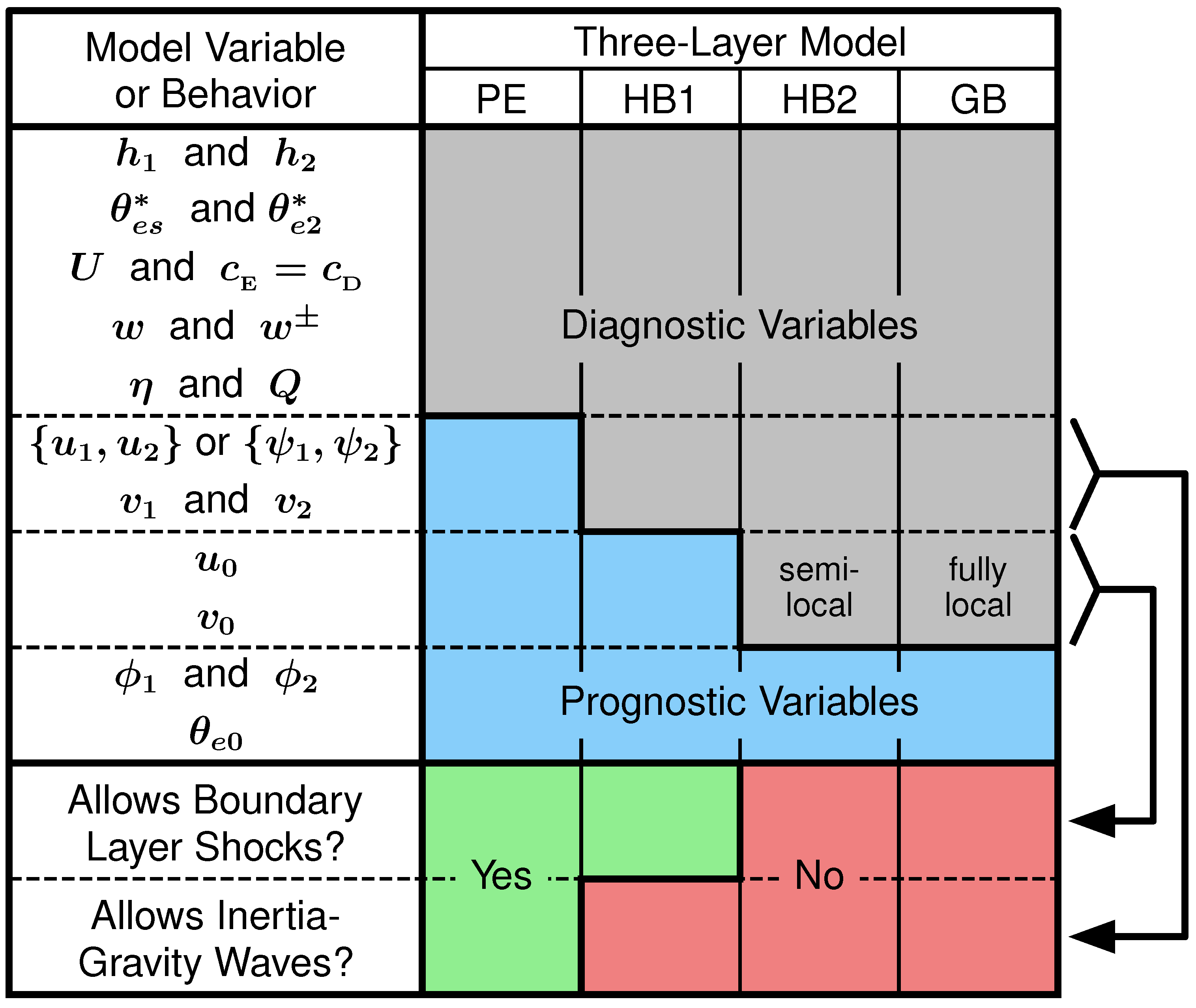
A comparison of the four models is given in Figure 2. The dependent variables of the four models are listed in the left column. The variables $h_1$, $h_2$, ${\theta }_{es}^{\ast }$, ${\theta }_{e2}^{\ast }$, U, $c_{{}_{\mathrm{D}}}$, $c_{{}_{\mathrm{E}}}$, w, $w^{\pm }$, $\eta$, and Q are diagnostic in all models, while the variables ${\varphi }_1$, ${\varphi }_2$, and ${\theta }_{e0}$ are prognostic in all models. The boundary layer wind components $u_0$ and $v_0$ are prognostic in the PE and HB1 models, but are diagnostic in the HB2 and GB models; this is related to the appearance of boundary layer shocks, as indicated by the inner arrow on the right. The radial and tangential wind components $u_1$, $u_2$, $v_1$, and $v_2$ are prognostic in the PE model but are diagnostic in the HB1, HB2 and GB models; this is related to the occurrence of propagating inertia-gravity waves, as indicated by the outer arrow on the right.

Through a comparison of the GB model Equations (Table 4) with the HB2 model Equations (Table 3), it is apparent that the only difference in the model equations is the more general, nonlocal boundary layer dynamics of the HB2 model. However, this difference leads to significant changes to the tropical cyclone life cycles simulated by the two models. These result from different Ekman pumping distributions. To illustrate these differences, Ooyama made comparison runs [1] using the constants listed in Table 5, the initial condition ${\varphi }_2(r,0)=0$, and with the initial ${\varphi }_1(r,0)$ in gradient balance with

$$v_1(r,0)=\widehat{v}\left(\frac{2(r/\widehat{r})}{1+{(r/\widehat{r})}^2}\right),$$

(20)

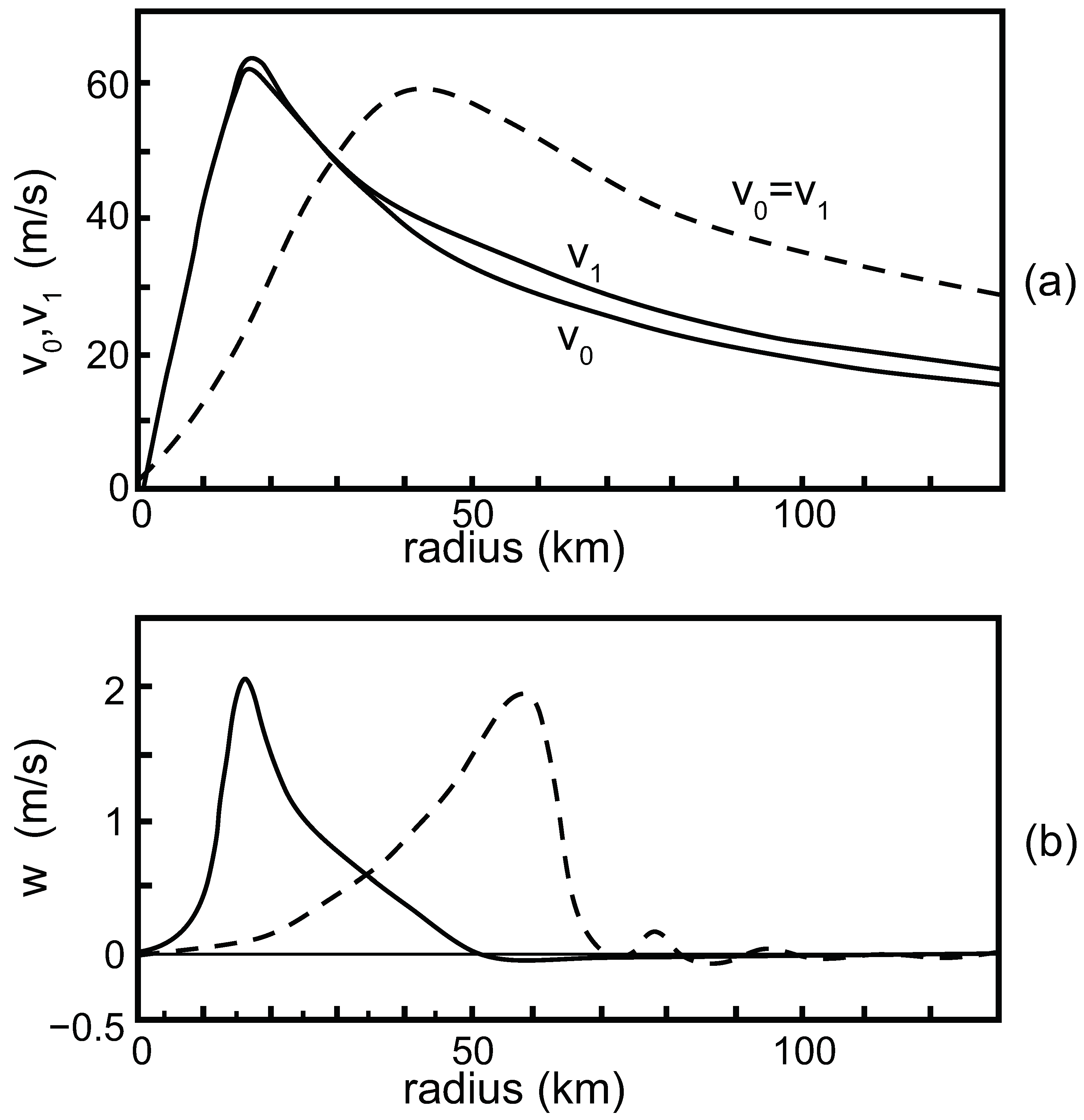
where the constants $\widehat{r}$ and $\widehat{v}$ are also given in Table 5. The initial condition on ${\theta }_{e0}(r,0)$ is determined from $\eta (r,0)=2$. Ooyama found in a numerical test that the values of $u_0$ and $v_0$ within 50 km from the vortex center are not influenced very much by their values outside 100 km. Solutions from HB2 are plotted as the solid curves in Figure 3 below (adapted from [1], Figure 2) and show three features found in later modeling studies [9,10,11,12,19] and also in observations of Hurricane Hugo [20]: (1) Subgradient boundary layer tangential flow outside the radius of maximum wind; (2) Supergradient boundary layer tangential flow near the radius of maximum wind; (3) Maximum Ekman pumping at a much smaller radius than in the GB model, resulting in a tighter vortex that intensifies more rapidly. As shown in Figure 3, the GB model produces an Ekman pumping with a 2 m s${}^{-1}$ maximum at $r\approx 60$ km with a sharp edge on the outside of the eyewall, while the HB2 model produces an Ekman pumping that maximizes at $r\approx 15$ km with a sharp edge on the inside of the eyewall. This difference is due to the $u_0(\partial u_0/\partial r)$ term in the HB2 model, i.e., to the nonlocal character of the boundary layer dynamics in HB2. This term leads to a nearly discontinuous behavior of the boundary layer radial inflow near $r\approx 15$ km, and hence the maximum Ekman pumping there. This behavior of $u_0$ in the HB2 model indicates the danger of formulating the nonlocal boundary layer dynamics without horizontal diffusion terms. If, without horizontal diffusion, the $u_0(\partial u_0/\partial r)$ term leads to the formation of a shock, the derivatives in the boundary layer equations can cease to exist, and the equations are no longer a useful description of the physics near the shock. This situation can be addressed by fitting in a shock condition or using horizontal diffusion to prevent multivalued radial inflow. The latter was the approach originally suggested by von Neumann and Richtmyer [21].

Table 5. Specified constants for the GB and HB2 model runs shown in Figure 3. Note that the large value of the initial average vorticity inside $\widehat{r}$, given by $2\widehat{v}/\widehat{r}=8f$, makes linear CISK theory (see Section 8 and references [2,22]) of limited use.

Parameter	Value	Parameter	Value
$ϵ$	0.9	$h_0$	1000 m
$\sigma =1-ϵ$	0.1	${\overline{h}}_1$	5000 m
g	9.81 m s${}^{-2}$	${\overline{h}}_2$	5000 m
f	$5\times {10}^{-5}$ s${}^{-1}$	${\overline{\theta }}_{es}^{\ast }$	372 K
$c_p$	1004.5 J kg${}^{-1}$ K${}^{-1}$	${\overline{\theta }}_{e2}^{\ast }$	342 K
$\mu$	$5\times {10}^{-4}$ m s${}^{-1}$	${\theta }_{e1}$	332 K
K	1000 m${}^2$ s${}^{-1}$	$\widehat{v}$	10 m s${}^{-1}$
$Q^{-}$	0 m s${}^{-1}$	$\widehat{r}$	50 km

Table 5. Specified constants for the GB and HB2 model runs shown in Figure 3. Note that the large value of the initial average vorticity inside $\widehat{r}$, given by $2\widehat{v}/\widehat{r}=8f$, makes linear CISK theory (see Section 8 and references [2,22]) of limited use.

Parameter	Value	Parameter	Value
$ϵ$	0.9	$h_0$	1000 m
$\sigma =1-ϵ$	0.1	${\overline{h}}_1$	5000 m
g	9.81 m s${}^{-2}$	${\overline{h}}_2$	5000 m
f	$5\times {10}^{-5}$ s${}^{-1}$	${\overline{\theta }}_{es}^{\ast }$	372 K
$c_p$	1004.5 J kg${}^{-1}$ K${}^{-1}$	${\overline{\theta }}_{e2}^{\ast }$	342 K
$\mu$	$5\times {10}^{-4}$ m s${}^{-1}$	${\theta }_{e1}$	332 K
K	1000 m${}^2$ s${}^{-1}$	$\widehat{v}$	10 m s${}^{-1}$
$Q^{-}$	0 m s${}^{-1}$	$\widehat{r}$	50 km

A particular limitation of the Ooyama (1969) cumulus parameterization scheme is the assumption that, if the column is conditionally unstable, the total cloud base vertical mass flux due to deep convection is equal to the vertical mass flux associated with the larger-scale horizontal convergence in the frictional boundary layer. Later studies showed that this assumption is not consistent with observations and with non-hydrostatic, full-physics models. For example, Yanai et al. [23] performed a heat and moisture budget analysis using an array of five radiosonde stations in the Marshall Islands, which are located in the tropical Pacific ITCZ. From the apparent heat source $Q_1$ and the apparent moisture sink $Q_2$, and using a simple bulk cloud model, Yanai et al. found that for cloud clusters in the ITCZ region, the total cloud base vertical mass flux is much larger than the vertical mass flux associated with the horizontal convergence in the frictional boundary layer. This conclusion about the vertical convective mass flux at the top of the boundary layer in weak tropical disturbances has been confirmed by several other observational studies, for example, [24,25,26]. However, as found by Smith et al. [27] using the full-physics CM1 model [28], this may not be the case for hurricanes and typhoons in their mature and decaying phases.

In order to remove some of the limitations of the Ooyama model, Zhu et al. [29] developed a three-layer, $\sigma$-coordinate tropical cyclone model with the option of explicit moist physics or different types of parameterized moist physics. The parameterized moist physics is primarily based on generalizations of the parameterization scheme designed by Arakawa [30] for the original 3-layer version of the UCLA general circulation model. An axisymmetric version of the Zhu et al. model was explored by Nguyen et al. [31], with follow-up studies carried out by Zhu and Smith [32,33], and Zhu et al. [34]. Together, these papers clarify the roles of shallow convection, precipitation-cooled downdrafts, and the vertical transport of momentum by deep convection on the dynamics of tropical cyclone intensification. Another family of simple hurricane models, not reviewed here, is the Maximum Potential Intensity (MPI) family first proposed by Emanuel [35,36,37] to help understand the air–sea interaction aspects and the finite amplitude and steady-state aspects of tropical cyclones. An extensive review of the MPI models and their use in understanding the basic intensification process and longer-term evolution of tropical cyclones can be found in recent reviews by Smith and Montgomery [38,39].

It is interesting to note that the family of models defined in Table 1, Table 2, Table 3 and Table 4 and summarized in Figure 2 has been organized in an unconventional manner. In the conventional organization (for example with community models such as WRF) all members of the family have the same dry dynamical core but have a variety of choices for the parameterized moist physics and air–sea interaction. In contrast, the four models in Table 1, Table 2, Table 3 and Table 4 and Figure 2 all have the same parameterized moist physics and air–sea interaction but have four different choices for the dry dynamical core. These two approaches to the organization of model families seem complementary and useful for helping understand the physics of tropical cyclones.

Other extensions of the four models listed in Table 1, Table 2, Table 3 and Table 4 have been described by Bliss [40] and DeMaria and Schubert [41], who relaxed the axisymmetric and balanced assumptions and formulated the three-dimensional (spectral) problem on a middle latitude $\beta$-plane to simulate storm motion. As another extension, DeMaria and Schubert [42,43] have formulated a generalized version of the axisymmetric PE model (Table 1) in order to apply the concepts of nonlinear normal mode analysis and initialization to the hurricane problem. The four models listed in Table 1, Table 2, Table 3 and Table 4 have no explicit thermodynamics, which at first sight seems problematic for a model of a phenomenon that involves latent heat release. However, DeMaria and Pickle [3] have shown that a model with explicit thermodynamics, if formulated in terms of isentropic layers, is almost mathematically equivalent to the incompressible layer model. The most complete comparisons of the four models of Table 1, Table 2, Table 3 and Table 4, along with several additional refinements, were given by Frisius and Lee [8], who performed numerical integrations that were, in the core region, twenty times the resolution (0.25 km vs. 5 km) used by Ooyama. Their results show additional fine structure and generally confirm the coarser resolution results shown in Figure 3.

The PE model described in Table 1 is not the only one of the four models that can be generalized to three dimensions. However, the generalizations of HB1, HB2, and GB to three dimensions can become somewhat complicated. The reason is that these involve generalizations of the classic $\omega$-equation of quasi-geostrophic theory, which is based on the selective use of the simplest relation between the wind and mass fields. This quasi-geostrophic $\omega$-equation is not valid for the inner core regions of intense tropical cyclones because of the large Rossby numbers found for the highly curved flows in the core. More general $\omega$-equations that are valid for the high Rossby number flows in tropical cyclones have been derived by Arakawa [44], Thompson [45,46], and Shapiro and Montgomery [47]. These arguments are based on generalizations of gradient wind balance, e.g., on the nonlinear balance equation in the derivations of Arakawa and Thompson and on asymmetric balance in the derivation of Shapiro and Montgomery. These generalized $\omega$-equations yield fully three-dimensional formulas for local inertial stability and local Rossby length. These second-order, elliptic, $\omega$-equations have the potential to provide diagnostic tools for a better understanding of such problems as the role of large-scale vertical wind shear on tropical cyclone structure and intensity change.

In closing, it is interesting to note that simple axisymmetric models have greatly expanded our understanding of tropical cyclone dynamics. For additional research that illustrates the rich history of these (and related models), see the studies by Emanuel [48,49], Shapiro [50], Camp and Montgomery [51], Smith and Vogl [10], Smith and Montgomery [52], Schecter and Dunkerton [53], Schecter [54,55], and Frisius et al. [56]. In many scientific fields, there is a tendency for the simplest models to experience a phase in which they yield new, remarkable physical insights (e.g., the Bohr model of the hydrogen atom, the Eady model of baroclinic instability, and the Ooyama model of tropical cyclones). Later, these simple models are used less in the research literature but are still very useful for introducing students to basic concepts. Although the simple family of tropical cyclone models described in Table 1, Table 2, Table 3 and Table 4 and Figure 2 may be entering their pedagogic phase, they may still prove useful in providing an increased understanding of the remarkable inner-core, lower-tropospheric structures observed in intense storms such as Hurricanes Hugo [20] and Patricia [57].

References

- Ooyama, K. Numerical simulation of tropical cyclones with an axisymmetric model. In Proceedings of the WMO/IUGG Symposium on Numerical Weather Prediction, Tokyo, Japan, 26 November–4 December 1968; Japan Meteorological Agency: Minato, Tokyo, 1969. Session III. pp. 81–88. [Google Scholar]
- Ooyama, K. Numerical simulation of the life cycle of tropical cyclones. J. Atmos. Sci. 1969, 26, 3–40. [Google Scholar] [CrossRef]
- DeMaria, M.; Pickle, J.D. A simplified system of equations for simulation of tropical cyclones. J. Atmos. Sci. 1988, 45, 1542–1554. [Google Scholar] [CrossRef]
- Eliassen, A. Slow thermally or frictionally controlled meridional circulation in a circular vortex. Astrophys. Norv. 1951, 5, 19–60. [Google Scholar]
- Greenspan, H.P.; Howard, L.N. On a time-dependent motion of a rotating fluid. J. Fluid Mech. 1963, 17, 385–404. [Google Scholar] [CrossRef]
- Greenspan, H.P. The Theory of Rotating Fluids; Cambridge University Press: Cambridge, UK, 1968; 325p. [Google Scholar]
- Eliassen, A.; Lystad, M. The Ekman layer of a circular vortex: A numerical and theoretical study. Geophys. Norv. 1977, 31, 1–16. [Google Scholar]
- Frisius, T.; Lee, M. The impact of gradient wind imbalance on tropical cyclone intensification within Ooyama’s three-layer model. J. Atmos. Sci. 2016, 73, 3659–3679. [Google Scholar] [CrossRef]
- Kepert, J.D. Slab- and height-resolving models of the tropical cyclone boundary layer. Part II: Why the simulations differ. Q. J. R. Meteorol. Soc. 2010, 136, 1700–1711. [Google Scholar] [CrossRef]
- Smith, R.K.; Vogl, S. A simple model of the hurricane boundary layer revisited. Q. J. R. Meteorol. Soc. 2008, 134, 337–351. [Google Scholar] [CrossRef]
- Williams, G.J.; Taft, R.K.; McNoldy, B.D.; Schubert, W.H. Shock-like structures in the tropical cyclone boundary layer. J. Adv. Model. Earth Syst. 2013, 5, 338–353. [Google Scholar] [CrossRef]
- Slocum, C.J.; Williams, G.J.; Taft, R.K.; Schubert, W.H. Tropical cyclone boundary layer shocks. arXiv 2014, arXiv:1405.7939. [Google Scholar]
- Tsujino, S.; Kuo, H.C. Potential vorticity mixing and rapid intensification in the numerically simulated Supertyphoon Haiyan (2013). J. Atmos. Sci. 2020, 77, 2067–2090. [Google Scholar] [CrossRef] [Green Version]
- Schubert, W.H.; Alworth, B.T. Evolution of potential vorticity in tropical cyclones. Q. J. R. Meteorol. Soc. 1987, 113, 147–162. [Google Scholar] [CrossRef]
- Möller, J.D.; Smith, R.K. The development of potential vorticity in a hurricane-like vortex. Q. J. R. Meteorol. Soc. 1994, 120, 1255–1265. [Google Scholar] [CrossRef]
- Hausman, S.A.; Ooyama, K.V.; Schubert, W.H. Potential vorticity structure of simulated hurricanes. J. Atmos. Sci. 2006, 63, 87–108. [Google Scholar] [CrossRef] [Green Version]
- Martinez, J.; Bell, M.M.; Rogers, R.F.; Doyle, J.D. Axisymmetric potential vorticity evolution of Hurricane Patricia (2015). J. Atmos. Sci. 2019, 76, 2043–2063. [Google Scholar] [CrossRef] [Green Version]
- Hendricks, E.A.; Vigh, J.L.; Rozoff, C.M. Forced, balanced, axisymmetric shallow water model for understanding short-term tropical cyclone intensity and wind structure changes. Atmosphere 2021, 12, 1308. [Google Scholar] [CrossRef]
- Kepert, J.D. Slab- and height-resolving models of the tropical cyclone boundary layer. Part I: Comparing the simulations. Q. J. R. Meteorol. Soc. 2010, 136, 1686–1699. [Google Scholar] [CrossRef]
- Marks, F.D.; Black, P.G.; Montgomery, M.T.; Burpee, R.W. Structure of the eye and eyewall of Hurricane Hugo (1989). Mon. Weather Rev. 2008, 136, 1237–1259. [Google Scholar] [CrossRef] [Green Version]
- von Neumann, J.; Richtmyer, R.D. A method for the numerical calculation of hydrodynamic shocks. J. Appl. Phys. 1950, 21, 232–237. [Google Scholar] [CrossRef]
- Charney, J.G.; Eliassen, A. On the growth of the hurricane depression. J. Atmos. Sci. 1964, 21, 68–75. [Google Scholar] [CrossRef]
- Yanai, M.; Esbensen, S.; Chu, J.H. Determination of bulk properties of tropical cloud clusters from large-scale heat and moisture budgets. J. Atmos. Sci. 1973, 30, 611–627. [Google Scholar] [CrossRef]
- Gray, W.M. Cumulus convection and larger scale circulations I. Broadscale and mesoscale considerations. Mon. Weather Rev. 1973, 101, 839–855. [Google Scholar] [CrossRef]
- Lopez, R.E. Cumulus convection and larger scale circulations II. Cumulus and mesoscale interactions. Mon. Weather Rev. 1973, 101, 856–870. [Google Scholar] [CrossRef]
- Ogura, Y.; Cho, H.R. Diagnostic determination of cumulus cloud populations from observed large-scale variables. J. Atmos. Sci. 1973, 30, 1276–1286. [Google Scholar] [CrossRef]
- Smith, R.K.; Kilroy, G.; Montgomery, M.T. Tropical cyclone life cycle in a three-dimensional numerical simulation. Q. J. R. Meteorol. Soc. 2021, 147, 3373–3393. [Google Scholar] [CrossRef]
- Bryan, G.H.; Fritsch, J.M. A benchmark simulation for moist nonhydrostatic numerical models. Mon. Weather Rev. 2002, 130, 2917–2928. [Google Scholar] [CrossRef]
- Zhu, H.; Smith, R.K.; Ulrich, W. A minimal three-dimensional tropical cyclone model. J. Atmos. Sci. 2001, 58, 1924–1944. [Google Scholar] [CrossRef]
- Arakawa, A. Parameterization of cumulus convection. In Proceedings of the WMO/IUGG Symposium on Numerical Weather Prediction, Tokyo, Japan, 26 November–4 December 1968; Japan Meteorological Agency: Minato, Tokyo, 1969. Session IV. pp. 1–6. [Google Scholar]
- Nguyen, C.M.; Smith, R.K.; Zhu, H.; Ulrich, W. A minimal axisymmetric hurricane model. Q. J. R. Meteorol. Soc. 2002, 128, 2641–2661. [Google Scholar] [CrossRef]
- Zhu, H.; Smith, R.K. The importance of three physical processes in a three-dimensional tropical cyclone model. J. Atmos. Sci. 2002, 59, 1825–1840. [Google Scholar] [CrossRef]
- Zhu, H.; Smith, R.K. Effects of vertical differencing in a minimal hurricane model. Q. J. R. Meteorol. Soc. 2003, 129, 1051–1069. [Google Scholar] [CrossRef]
- Zhu, H.; Ulrich, W.; Smith, R.K. Ocean effects on tropical cyclone intensification and inner-core asymmetries. J. Atmos. Sci. 2004, 61, 1245–1258. [Google Scholar] [CrossRef]
- Emanuel, K.A. An air–sea interaction theory for tropical cyclones. Part I: Steady-state maintenance. J. Atmos. Sci. 1986, 43, 585–604. [Google Scholar] [CrossRef]
- Emanuel, K.A. The finite-amplitude nature of tropical cyclogenesis. J. Atmos. Sci. 1989, 46, 3431–3456. [Google Scholar] [CrossRef]
- Emanuel, K.A. The behavior of a simple hurricane model using a convective scheme based on subcloud-layer entropy equilibrium. J. Atmos. Sci. 1995, 52, 3960–3968. [Google Scholar] [CrossRef]
- Montgomery, M.T.; Smith, R.K. Mininal conceptual models for tropical cyclone intensification. Trop. Cyclone Res. Rev. 2022, 11, 61–75. [Google Scholar] [CrossRef]
- Smith, R.K.; Montgomery, M.T. Tropical Cyclones: Observations and Basic Processes; Elsevier: Amsterdam, The Netherlands, 2023. [Google Scholar]
- Bliss, V.L. Numerical Simulation of Tropical Cyclone Genesis. Ph.D. Thesis, Department of Atmospheric Science, University of Washington, Seattle, WA, USA, 1980; 268p. [Google Scholar]
- DeMaria, M.; Schubert, W.H. Experiments with a spectral tropical cyclone model. J. Atmos. Sci. 1984, 41, 901–924. [Google Scholar] [CrossRef]
- Schubert, W.H.; DeMaria, M. Axisymmetric, primitive equation, spectral tropical cyclone model. Part I: Formulation. J. Atmos. Sci. 1985, 42, 1213–1224. [Google Scholar] [CrossRef]
- DeMaria, M.; Schubert, W.H. Axisymmetric, primitive equation, spectral tropical cyclone model. Part II: Normal mode initialization. J. Atmos. Sci. 1985, 42, 1225–1236. [Google Scholar] [CrossRef]
- Arakawa, A. Non-geostrophic effects in the baroclinic prognostic equations. In Proceedings of the International Symposium on Numerical Weather Prediction, Tokyo, Japan, 7–13 November 1960; The Meteorological Society of Japan: Tokyo, Japan, 1962; pp. 161–175. [Google Scholar]
- Thompson, P.D. A theory of large-scale disturbances in non-geostrophic flow. J. Meteorol. 1956, 13, 251–261. [Google Scholar] [CrossRef]
- Thompson, P.D. A short-range prediction scheme based on conservation principles and the generalized balance condition. Contrib. Atmos. Phys. 1980, 53, 256–263. [Google Scholar]
- Shapiro, L.J.; Montgomery, M.T. A three-dimensional balance theory for rapidly rotating vortices. J. Atmos. Sci. 1993, 50, 3322–3335. [Google Scholar] [CrossRef]
- Emanuel, K.A. Tropical cyclones. Annu. Rev. Earth Planet. Sci. 2003, 31, 75–104. [Google Scholar] [CrossRef]
- Emanuel, K.A. 100 years of progress in tropical cyclone research. Meteorol. Monogr. 2018, 59, 15.1–15.68. [Google Scholar] [CrossRef]
- Shapiro, L.J. Hurricane vortex motion and evolution in a three-layer model. J. Atmos. Sci. 1992, 49, 140–153. [Google Scholar] [CrossRef]
- Camp, J.P.; Montgomery, M.T. Hurricane maximum intensity: Past and present. Mon. Weather Rev. 2001, 129, 1704–1717. [Google Scholar] [CrossRef]
- Smith, R.K.; Montgomery, M.T. Balanced boundary layers used in hurricane models. Q. J. R. Meteorol. Soc. 2008, 134, 1385–1395. [Google Scholar] [CrossRef] [Green Version]
- Schecter, D.A.; Dunkerton, T.J. Hurricane formation in diabatic Ekman turbulence. Q. J. R. Meteorol. Soc. 2009, 135, 823–838. [Google Scholar] [CrossRef]
- Schecter, D.A. Hurricane intensity in the Ooyama (1969) paradigm. Q. J. R. Meteorol. Soc. 2010, 136, 1920–1926. [Google Scholar] [CrossRef]
- Schecter, D.A. Evaluation of a reduced model for investigating hurricane formation from turbulence. Q. J. R. Meteorol. Soc. 2011, 137, 155–178. [Google Scholar] [CrossRef]
- Frisius, T.; Schönemann, D.; Vigh, J. The impact of gradient wind imbalance on potential intensity of tropical cyclones in an unbalanced slab boundary layer model. J. Atmos. Sci. 2013, 70, 1874–1890. [Google Scholar] [CrossRef]
- Rogers, R.F.; Aberson, S.; Bell, M.M.; Cecil, D.J.; Doyle, J.D.; Kimberlain, T.B.; Morgerman, J.; Shay, L.K.; Velden, C. Rewriting the tropical record books: The extraordinary intensification of Hurricane Patricia (2015). Bull. Am. Meteorol. Soc. 2017, 98, 2091–2112. [Google Scholar] [CrossRef]
Figure 1.
Schematic diagram of the axisymmetric, three-layer, f-plane family of models. The constant density in the lower two layers is , while the constant density in the upper layer is , with . The thicknesses of the layers are , , and , with a specified constant, and with and functions of . The radial velocity components are , , and , and the radial mass fluxes are , , and . The tangential velocity components are , , and . The surface stress drives the boundary layer radial inflow, which results in boundary layer pumping () in the inner region and boundary layer suction () in the outer region. Diabatic processes are parameterized through the mass transport terms and . Adapted from ([2], Figure 1).
Figure 2.
Comparison of the diagnostic and prognostic variables from the four models. The left column lists the model variables, all of which are functions of r and t. For the PE model, the bottom nine variables are prognostic, and all the remaining variables (above them in the table) are diagnostic. For the HB1 model, only the bottom five variables are prognostic, and four variables ( or , , and ) that are prognostic for the PE model are now diagnostic. For the HB2 and GB models, just the bottom three variables are prognostic with two variables ( and ) that are prognostic for the PE and HB1 models now being diagnostic. The PE model allows propagating inertia-gravity waves in the upper two layers, while the other three models filter these waves because the radial components and are determined diagnostically, as indicated by the outer arrow on the right. Because of the form of their and equations, the PE and HB1 models allow the formation of well-defined boundary layer shocks, as indicated by the inner arrow on the right.
Figure 3.
Comparison of the tangential winds and (a) and the Ekman pumping w (b) for the gradient balanced model (GB, dashed lines) and the second hybrid model (HB2, solid lines) at h for a typical life cycle experiment. The vortex in HB2 is tighter and has gone through a more rapid intensification than the vortex in GB. This difference in structure and intensification rate is due to the striking differences in Ekman pumping, with the GB model having its 2 m s maximum w at km and the HB2 model having a similar maximum but at km. This illustrates the fundamental importance of the term in the radial equation of boundary layer motion in the HB2 model. Note that the boundary layer tangential flow in the HB2 model is slightly subgradient for km and slightly supergradient for km. This subgradient/supergradient effect can be more apparent in strong storms such as Hurricane Hugo (see [11,20]). Adapted from ([1], Figure 2).
Disclaimer/Publisher’s Note: The statements, opinions and data contained in all publications are solely those of the individual author(s) and contributor(s) and not of MDPI and/or the editor(s). MDPI and/or the editor(s) disclaim responsibility for any injury to people or property resulting from any ideas, methods, instructions or products referred to in the content. |
© 2023 by the authors. Licensee MDPI, Basel, Switzerland. This article is an open access article distributed under the terms and conditions of the Creative Commons Attribution (CC BY) license (https://creativecommons.org/licenses/by/4.0/).
Share and Cite
MDPI and ACS Style
Schubert, W.H.; Taft, R.K.; Slocum, C.J. A Simple Family of Tropical Cyclone Models. Meteorology 2023, 2, 149-170. https://doi.org/10.3390/meteorology2020011
AMA Style
Schubert WH, Taft RK, Slocum CJ. A Simple Family of Tropical Cyclone Models. Meteorology. 2023; 2(2):149-170. https://doi.org/10.3390/meteorology2020011
Chicago/Turabian StyleSchubert, Wayne H., Richard K. Taft, and Christopher J. Slocum. 2023. "A Simple Family of Tropical Cyclone Models" Meteorology 2, no. 2: 149-170. https://doi.org/10.3390/meteorology2020011