1. Introduction
The use of renewable energy sources, including solar energy, is no longer a novelty today. The commissioning of recovery equipment, solar panels and solar collectors used to be a kind of environmental investment. These could ensure that we would produce electricity with less carbon dioxide emissions or produce domestic hot water. Today, however, the opportunities to reduce our energy dependency deserve more attention. Locally produced energy also provides the security of supply, both on an industrial and domestic scale. By now, solar solutions, previously considered very expensive, have become competitive in one fell swoop. The reasons for this are the sharp rise in fossil energy prices and the severe economic crisis that is already well foreseen. Furthermore, we need electricity even more, because we can hardly imagine our way of life today without it.
In 2020, there were already 1407 MW of photovoltaic-installed energy capacity in the Hungarian electricity system. This is 14.2% of our total power plant capacity. This year, Hungarian solar parks generated a total of 2419 TWh of electricity, which is already 6.94% of the total electricity production. This is at least three times more than electricity generated from wind energy in 2020 (654,687 GWh; 1.88%). The amount of electricity produced with this solar energy grew by far the fastest in Hungary compared to 2019 [
1].
The current renewable energy support system (METÁR) operated beginning on 1 January 2017. Prior to 2020, new renewable investments were supported with a mandatory takeover price. In 2020, however, the support could only be applied for in the form of a green premium-type entitlement awarded through a tender procedure [
2]. In the premium system, the producer sells the electricity himself and receives the aid above the market reference price.
Under the premium scheme, producers have to bear the costs of deviating from the schedule. The accuracy of the production forecast will be important and really interesting here. Hopefully, despite the increasingly complex regulations, the construction of solar parks will continue in the future. From 1 January 2022, they could expect an average feed-in price of HUF 35.54/kWh (KÁT). At the same time, solar panels of less than 1 MW licensed after 2020 can already receive an average subsidy of HUF 28.44/kWh. For the units included in the balance sheet of KÁT, forecasting and maintaining the schedule is a serious challenge and difficulty. MAVIR (Hungarian Electricity Transmission System Operator Private Limited Company) determines deviations from the schedule and invoices regulatory surcharges to the members of the KÁT balance group. The official price only applies to the actual production. Producers must provide a 12-month rolling forecast by the 7th day of each month and have the opportunity to change the daily forecast for the previous day and the same day [
3]. However, despite the challenges, managing weather-dependent performance is possible in several ways.
The method presented below can help energy producers make a monthly rolling forecast. Before this, firstly we will present what we consider to be the most important nodes of solar radiation research in Hungary. Next, we present some examples of the statistical models most commonly used by researchers worldwide.
2. Measurement and Estimation of Global Radiation in Hungary
According to the meteorological radiation theory, global radiation refers to the amount of energy that arrives from the total solar radiation to the surface unit of the horizontal plane during a unit of time [
4]. The radiation energy coming from the Sun to the Earth’s surface is the most important climate-shaping factor and its place in the energy mix is also very significant.
In Hungary, the continuous or network-like measurement of solar radiation began much later than the measurement of other climatic elements. It began in the 1930s, mainly due to the lack of suitable instruments. However, after the installation of the radiation measuring instruments, the data were not always accurate and sufficient due to their placement and authentication problems, the technical errors that occurred, and the small number of comparisons with the absolute instrument. At the beginning of the 1970s, the Robitzsch-type instruments were replaced by more modern equipment, but at the same time, the number of radiation-measuring stations significantly decreased [
5]. After 2001, with the installation of automatic measuring stations, their number also increased. Currently, the Hungarian Meteorological Service (HMS/OMSz) network has 46 radiation measurement stations with reliable pyranometers providing 10-min data [
6].
The replacement of data from stations operating irregularly in space and time and their homogenization after changing instruments necessitated the development of calculation and estimation methods based on the measured value of other climate elements. These methods or their improved versions can still be successfully used today for spatial and temporal extrapolation of the measured data of global radiation. Just think of the homogenized data used in the study of climate change.
The most reliable calculation method is based on the close relationship between sunshine duration and irradiance. This is based on Ångström’s formula [
7], the input data of which, in addition to the relative duration of sunshine, are also the value of global radiation in the case of clear skies and a constant characteristic of the given area. By eliminating the latter two or determining them based on measurements, the equation becomes stochastic.
The Hungarian method of calculating global radiation from the duration of sunshine was published in Ref. [
8]. The basis of the method is the linear stochastic relationship between the two elements, with monthly regression coefficients. Using this method, the long-term (1901–1950) averages of global radiation in Hungary were determined and their territorial distribution was analyzed [
9].
After supplementing and homogenizing the data of the radiation measuring stations, the first measured climatological data series on global radiation in Hungary was produced from the data of the period 1958–1972 [
4]. During the examined period, it was possible to collect measured data sets that could be considered complete from 13 stations. However, data from several stations were needed to compile the maps showing the average monthly and annual amounts. Where there was no radiation measurement, the daily amounts of global radiation were calculated/estimated from the data on the duration of sunlight and cloudiness. In addition to the maps, the frequency distribution, mean and standard deviation of the daily amounts were also determined monthly at the 13 stations.
From the study, we selected and examined the monthly frequency distributions, averages and standard deviations for Szeged. It could be observed that the distributions were already rearranged in the transitional months, i.e., the months preceding the seasons. This occurred markedly in the change in the interval containing the maximum frequency. The maximum value of the average global radiation for one day of the month could be observed in June and July and the minimum in December. This, of course, corresponded to Hungary’s climatic characteristics [
10].
Later, on an expanded database (1958–1982), the meteorological foundations of solar energy utilization in Hungary were laid [
11].
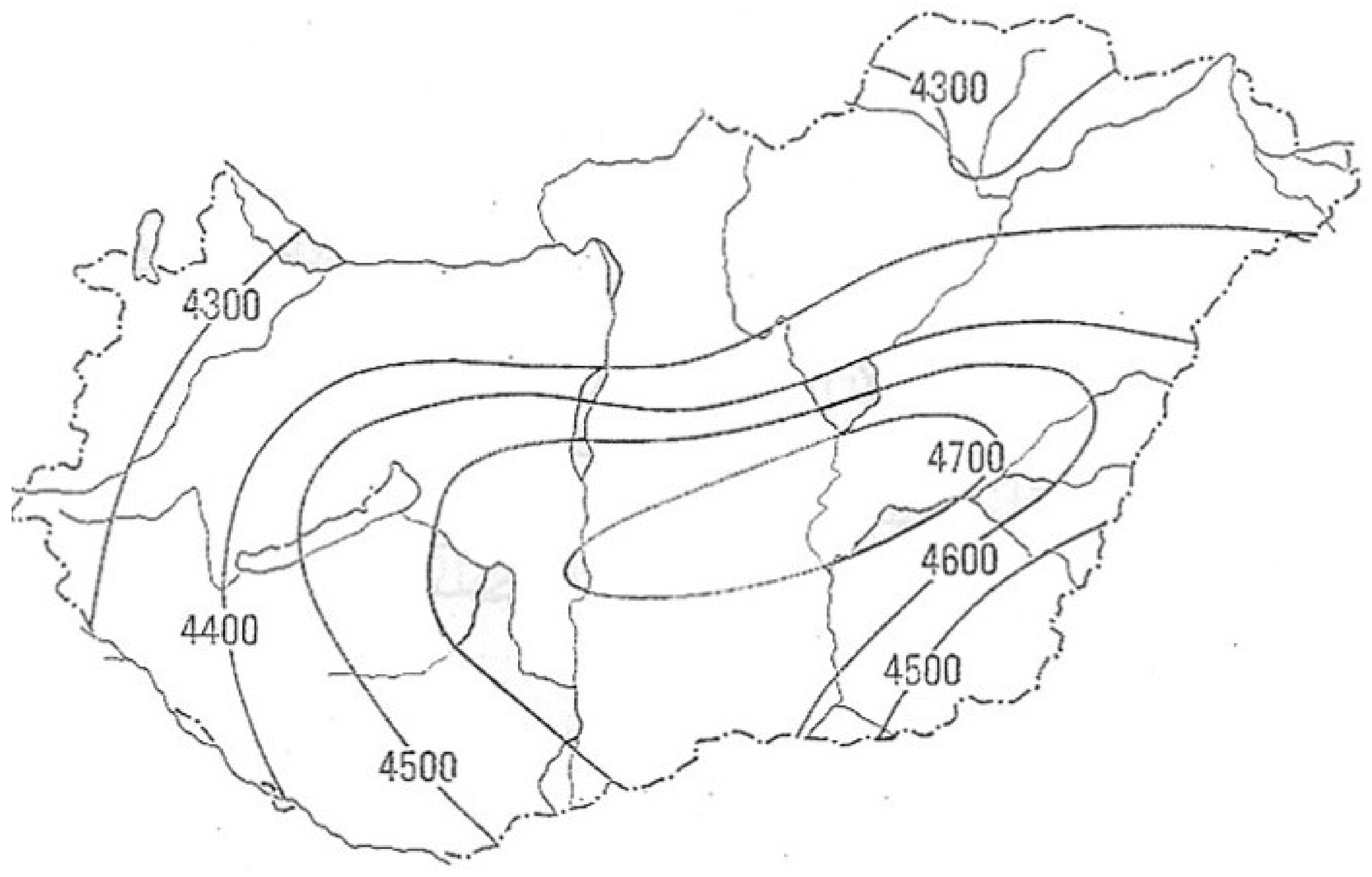
Figure 1 is from this study. The figure shows the territorial distribution of the average annual amounts of global radiation in Hungary in the currently accepted unit of measurement (MJm
−2). While the zonal distribution dominated on the previous, smaller database maps [
6], on this one (and also on the one made in 1976) the maximum was characterized by the closed area visible in the middle of the country. This could also be observed in the case of other climatic elements and refers to the basin nature of the climate of our country [
12]. However, this was not visible on the map appearing on the OMSz website [
10]. This may have been due to the smaller size of the database (2000–2009) or to changes in the country’s climate. The OMSz map shows a maximum exceeding 4900 MJm
−2 in the southeastern areas (around Szeged).
Scientific fields dealing with the various effects of atmospheric processes also have specific methods for determining and estimating global radiation.
On the Earth’s surface, the daily global radiation is a very important component of the mass and energy processes of the ecosystem, including in crop modeling. The lack of radiation data limits the use of crop models. In Ref. [
13], an efficient global radiation estimation method was further developed using the measured data of some meteorological stations covering Hungary. The method enabled crop modelers to use their models in locations where this was previously impossible due to the lack of measured solar radiation data.
The engine that maintains the hydrological cycle is the short-wave radiation coming from the Sun to the Earth’s surface. It is therefore necessary that its value can be estimated using simple tools in hydrological studies. The first step of the approximation method described in Ref. [
14] was the estimation of the deterministic value of extraterrestrial radiation reaching the outer surface of the atmosphere. The sum of daily energy was given in trigonometric form depending on the latitude and calendar day. By integrating this between appropriate limits, the annual, half-yearly or monthly energy amounts can also be calculated. When calculating the global radiation reaching the Earth’s surface from the extraterrestrial value, the effect of the random state of the atmosphere must be taken into account, which affects the absorption and reflection of the incoming energy. This can mostly be done by taking into account the value of the relative sunshine duration. Comparing several methods, the conclusion can be drawn that in order to reduce uncertainty, it is advisable to use only the two extreme values (1 and 0 relative sunshine duration) in hydrological studies. The intervening changes are estimated based on the precipitation amounts. It has been established that even the use of this simple method of estimation helped in connecting hydrological climate models. The goal is to find the simplest meteorological variables that can be used with good results to numerically characterize the triple relationship of precipitation–evaporation–runoff.
The method described in Ref. [
8] was further developed by Ref. [
15] in such a way that the statistical relationship between the amount of daily global radiation and the relative amount of sunlight was determined by a third-degree polynomial. In order to increase the accuracy of the approximation, the effects of cloudiness and vapor pressure were also taken into account through stochastic relationships.
Estimating the amount of global radiation from clouds became possible with the advent of meteorological satellites. Today, high temporal and spatial resolution measurements of these devices have become the main sources of radiation data [
6]. In the beginning, however, the three daily satellite images (cloud analysis map) were of course insufficient for climate analyses. Our meteorologists developed an empirical method, with the help of which they calculated the components of the radiation balance for the territory of Hungary, including the global radiation, from the recordings available every 8 h [
16]. The ultimate goal of their work was to forecast global radiation for a few days using satellite information. This is also very important for the better utilization of solar energy equipment. Today, Hungary is an associate member of EUMETSAT, the European organization responsible for the utilization of meteorological satellites. The task of the Climate Working Group of this organization is to produce high-quality databases suitable for examining climate change and to serve the needs of the solar energy sector.
The role of the amount of solar radiation estimated and predicted by meteorologists in the process of utilizing solar energy appears mainly in technical and energetic studies. However, the relationship between meteorology and solar energy utilization may be even more direct than this. For example, the meteorological laws that can be used to determine the solar radiation income of inclined surfaces (i.e., solar panel or solar collector) can be presented [
17].
Stochastic relationships between the daily global radiation and electricity generation from photovoltaic (PV) panels have also been investigated [
18]. The linear correlation coefficient of the horizontal PV output and the measured global radiation is 0.930, which proves a strong stochastic relationship between the two data sets. This correlation was also established in the case of the 45°, south-facing panel most often used in Hungary.
However, live, direct contact is also possible. The study of Tóth and Farkas (2021) [
19] presented a mathematical model of the operation of a solar collector system (solar collector, heat storage, pump). It was shown that it is possible to connect the Simulink-based (a simulation and model-based design environment) model to a meteorological database server as an external data source. The structure of the predictive control of the model and the results of the simulation were also presented. This computationally heavy control method can be used on today’s personal computers and can be extended.
3. Some Examples of the Most Commonly Used Statistical Models for Estimating Global Radiation
Statistical models now work as they do for other climate elements: they analyze the stochastic relationship between the calculated or older measured values of global radiation, as well as the simultaneously measured values of another climate element and the true (measured) amount.
The performance of the models is most often evaluated using the following statistical parameters: the root mean square error (RMSE), mean absolute bias error (MABE, MBE), mean absolute percentage error (MAPE, MPE) and the Nash–Sutcliffe Equation (NSE) (see, e.g., [
20]).
The models described in this chapter—unlike the model we developed—do not use older measured data in the model creation, only in the validation process. A striking example of this is in Ref. [
20]. In this paper, three simple day-of-the-year, global solar radiation models, which consider only the day of the year as the input values, were calibrated and verified with the measured data for the solar climate of Poland. As expected, the goodness of fit of the tested models, expressed by the determination coefficient, was slightly worse than in other climatic zones, yet it was maintained within 0.94–0.97 and could be considered satisfactory. Regarding the long-term monthly average daily solar radiation, the values of statistical error parameters (RMSE, MABE, MAPE) demonstrated slight differences between the tested models. More significant differences could be observed between the individual stations analyzed.
One possible way to model the amount and duration of solar radiation is to use astronomical laws instead of thermo- and hydrodynamic laws, taking into account the instantaneous, average or assumed value of the atmospheric status indicators. The majority of such models are based on the Ångström–Prescott formula. This formula is a linear relationship between the ratio of the measured global radiation (H) and extraterrestrial solar radiation (H
0), and the ratio of sunshine duration (S) and the astronomically possible sunshine duration (S
0) at a given point on the Earth’s surface in a day. The explicit form of the formula is:
where a and b are the regression constants. For a more detailed description of the formula and a possible way of determining the parameters included in it, see in Ref. [
21].
However, in the case of some models, the latter quotient is replaced by a formula dependent on extreme temperatures. These models assume that the difference between the maximum temperature and the minimum temperature is directly related to the extraterrestrial solar radiation received at the surface, since the temperature variable includes the radiation, humidity, cloudiness, latitude and topography of the study site. You can read about the Ångström–Prescott formula and the models derived from it in Refs. [
21,
22].
In the following, we selected from the application of the models listed in Refs. [
21,
22] or those similar to them.
Akinpelu et al. (2018) [
23]: Various climatic parameters have been used for developing empirical relations for predicting the monthly average global solar radiation. Among the existing correlations, the modified form of the Ångström-type regression equation is generally accepted. In this article, the investigated global radiation amount was modeled with the original formula (see Equation (1)). A possible way to calculate the a and b regression constants in the equation as well as the astronomical parameters was also provided. It was found that the model predicted the global solar radiation quite accurately in the studied locations. This was supported by comparing the values of standard statistical error parameters and linear correlations. It was concluded that the correlation proposed for these sites can be used successfully for the estimation of H for any location of Nigeria with similar meteorological characteristics.
Ben Jemaa et al. (2013) [
24]: The purpose of the paper was to evaluate the linear regression method commonly used by researchers in the past for the three models (linear, quadratic and cubic, see e.g., in Refs. [
21,
22,
25]) used to estimate the monthly and annual average global solar radiation from a location. The linear model was the Ångström–Prescott formula itself, in the quadratic model the quotient of the sunshine duration and the astronomically possible sunshine duration was also included in the square, and in the cubic model also in the cube. Comparative studies (linear regression) between the global solar radiations estimated from the three models and the measured values showed that all models gave very good results. According to the statistical parameters, MABE, MAPE and RMSE used to determinate the statistical test t, it could be seen that the estimated values of daily global radiation were in a favorable agreement with the measured values for all the models. However, the linear model had better performance than the two other models.
Muzathik et al. (2011) [
25]: In this study, the accuracy among the ten models was determined using the data measured at Kuala Terengganu (Malaysia) in the periods between 2004 and 2007. The first model was the original Ångström–Prescott formula. In addition to the extraterrestrial radiation, other models also only included the transformed quotient of the sunlight durations as input. The two, three or four regression constants were obtained using the curve fitting tool of MATLAB. These coefficients are subjected to a large variability according to the type of model. The values of the monthly mean daily global solar radiation intensity estimated using the 10 models were compared with the corresponding measured values. The statistical tests of MBE, MPE, RMSE, NES, r and
t-test were determined for the entire period. The
t-test function is now defined by the error parameters MBE and RMSE. The comparison between the different models according to the t value showed that the calculated t values were less than the critical t value except for model 10. These results showed that the models 1 to 9 had statistical significance. Therefore, the models are extremely recommended to estimate the monthly average daily global solar radiation for the Terengganu state areas and elsewhere in areas with similar climatic conditions where the radiation data are missing or unavailable.
Ihaddadene et al. (2019) [
26]: In this study, seven empirical models have been employed to estimate the daily average global solar radiation on the horizontal surface. These models used extreme temperatures (minimum and maximum). They were applied to three South Algerian sites. The validation of the models for predicting the daily global solar radiation was done using the regular statistical parameters. The results showed that the Bristow Campbell Model (see [
21,
22]) showed a better performance than the other models at all sites. Based on the results, a new model was proposed for each site. This model described the daily global solar radiations as a linear function of the extraterrestrial radiation and the sum of the maximum and minimum temperature. The coefficients of this model depended on the chosen site. It was applicable for three sites in Algeria. It is the best one in the series of the models studied. It allows for determining the evolution of the daily global solar radiation using only the extreme temperature values (maximum and minimum) in the south of Algeria.
Quansah et al. (2014) [
27]: The performances of both sunshine- and air temperature-dependent models for the estimation of the daily global solar radiation over Ghana and other tropical regions were evaluated and a comparison assessment of the models was carried out using measured data. Seven models were evaluated, five of which were based on the Ångström–Prescott relation and two on the Hargreaves and Samani (see both in Refs. [
21,
22]) models. Furthermore, an empirical model which also uses sunshine hours and air temperature measurements from the study site and its environs was proposed. The results showed that all the models could predict very well the pattern of the measured daily mean global radiation for the entire period of the study. A very good agreement was found between the measured radiations and the proposed models with a coefficient of determination within the range of 0.88–0.96. The results also revealed that the proposed models using sunshine hours and air temperature had the smallest values of MBE, MPE and RMSE.
Ghazouani et al. (2022) [
28]: This work investigated the performance of four temperature-based hybrid solar radiation models combining the parametric, statistical and satellite data approaches to estimate the global solar radiation on a horizontal surface. According to the obtained results, all developed models in this study performed well in predicting the monthly average daily global solar radiation on the horizontal surface. Accurate estimations with the highest accuracy and excellent values for the statistical error indicators (RMSE, MABE, MAPE) were compared with those of other models.
Gürel et al. (2023) [
29]: The climate-shaping role of global radiation and its place in the energy mix made it necessary for researchers to turn their attention to low-error estimates. Accordingly, it can be observed that various models have been continuously developed in the literature. This review article mainly dealt with the solar radiation works estimated using empirical models, time series, artificial intelligence algorithms and hybrid models. This study presented a detailed comparison of the different methods found in the literature used to estimate solar radiation. Among other things, it stated that the majority of the input parameters generally consist of the environmental and ecological input parameters such as the sunshine duration, relative humidity, ambient temperature, sunshine ratio, minimum, maximum and mean air temperature, Earth skin temperature, wind speed, wind direction, clear-sky estimates, satellite images, rainfall, atmospheric pressure, etc. In addition to these, many models also use astronomical parameters as input.
This conclusion is important and essential from the point of view of our article, because among the many models examined, there is no one whose input parameter is derived from the older measurements of global radiation.
4. Data and Methods
In addition to dynamic meteorological methods, purely statistical models also play an important role in predicting the various characteristics of climate elements. The dynamic models describe atmospheric movement systems of different scales with hydro-thermodynamic laws. The statistical estimation or forecasting is basically based on stochastic laws that can be deduced from climate data that are measured or observed over a long period of time.
Let us see two examples from Hungary.
Using Budapest’s monthly mean temperature data, [
30] searched for the optimal use of long-term averages. For the 12 months of the year, it was determined how many years’ averages give the best approximation for the following year. It was examined whether it was sufficient to recalculate the average values produced in this way every ten years. Here, therefore, the estimated and estimator values belonged to the same set.
In Ref. [
31], a statistical procedure was developed for the prediction of radiation fogs generated at the Budapest airport. First, the stochastic relationship between the aerological parameters used in the fog forecasting process and the generation of radiation fogs was examined. The average accuracy of the fog forecast based on this method was 84%. In this case, the estimated value and the estimator values are elements of different sets.
4.1. The Sliding Average Model
In the case of meteorological observations, the measured values of the climatic elements are usually recorded at regular times (i = 1, 2,…, (n − 1), n) within a given period. The exact sum (e.g., precipitation, global radiation) or average (e.g., wind speed, temperature) of the time series (daily, monthly…) obtained in this way can only be determined after the last measurement of the period. However, in some cases it may be necessary to estimate this amount or average with an acceptable error before the last measurement time.
Take, for example, one of the most difficult problems for wind farm operators, the preparation of a so-called “timetable” (schedule). This is an estimate of the amount of electricity produced every quarter of an hour the following day. This can be helped by telling us the probability of a decrease or increase in the average wind speed the next day (and with it the average daily wind power), or which of these two probabilities is greater. This requires an estimate of tomorrow’s average wind speed, the change of which into the next day has a very strong stochastic relationship with today’s average wind speed [
32].
However, the exact average daily speed can only be determined from hourly data at the end of the day. In order to use the estimate, this data should be known sooner, therefore an approximate value that can be calculated earlier has to be applied. The method intended to determine this value is presented in the following.
The problem can be generally stated as follows: the measured values of a climatic element are recorded at regular times (e.g., hourly, daily) during periods i = 1, 2, …, (n − 1), n. The exact average of this time series can only be determined after the measurement n. However, in some cases, it may be necessary to estimate this average before date n with an acceptable error.
The statistical model to be presented in the following was designed to solve the above problem. The bases of the model were published by Ref. [
32]. The database of the model is composed of a statistically sufficient measurement data matrix for a given climate element, the elements of which shall be
xi,
j. The general form of the matrix
xi,j is:
j: row index,
j = 1, 2, …, (
N − 1),
N,
i: column index,
i = 1, 2, …, (
n − 1),
n. Thus,
N can represent the number of days involved in processing and
n can be the number of measurements at equal intervals (e.g., hourly) per day.
At each measurement time (
i) the [
xi,j] elements of the so-called sliding averages matrix are counted per line (
j):
Thus, [
xi,j] represents the average calculated up to the measurement time
i of row
j,
i. e. [
xn,j] gives the total average of the line
j. Knowing this, the so-called relative sliding averages are obtained:
which is therefore the ratio of the average of the row up to time i and the average of the entire row. Their average—the so-called average relative sliding average—has to be calculated at each measurement time:
depends on the selected climate element and is presumably dependent on the location of the observation and the weather situation, as well as the season. Therefore, it is advisable to produce the average relative sliding average at a given location in addition to the entire database for certain subsets of this, e.g., by the macrosynoptic position group or situation, for the growing season, seasonally, etc.
The
parameter is used for testing the model and of course for its operative running, i.e., for the estimation of the exact series average outside the database of the given climatic element used in the formation of the model. The row averages [
xn,j] (e.g., the daily averages) are estimated from the sliding average [
xi,j] at measurement time i. The estimation is made by writing the average of
Ri,j instead of it in Equation (3), i.e.,
The estimated value of the total average therefore also depends on the time point from which the estimate is made.
Of course, a different parameter of the Ri distribution selected for the particular goal (i.e., mode) can also be used instead of in the course of the estimation.
In the course of the verification, estimation (4) at all times of all series is performed then—as [
xn,j] is known. The
average of the relative error of the estimations (in %) at the times is calculated from
Ei,j, where:
i.e., the relative error per estimate, hence:
Equation (6) measures the magnitude of the daily relative error, which is always positive or zero. If we also want to examine the sign of the relative error, we use the form of Equation (6) without the absolute value (their mean is denoted by ). Thus, we can examine for example, the proportion of underestimations and overestimations.
The detailed structure and application of the SLIDAV model to the problem described above is summarized in Ref. [
32]. The detailed analyses showed that by combining the daily average wind speed change and the sliding-average model, more important information about the wind climate of Hungary can be revealed. We hope these models will also help you create a schedule. In the case of a given wind farm, the application of the methods is much simpler, as the characteristics required for the operation of both models can be obtained from the long-term wind speeds measured there.
4.2. The Sliding-Sum Model
If the goal is to estimate the sum of the data matrices xi,j per row (e.g., the amount of monthly precipitation or global radiation), then we can omit averaging in Equation (2). The parameters of this model (SLIDSUM) are similar to the previous ones:
The total sum of
jth line:
Knowing this, we form the so-called relative sliding amounts:
The average relative sliding amount is:
The sum of the line
j is now estimated by entering the average
RSi,j in Equation (10), i.e.,
Equations (6) and (7) are modified as above for the verification and error calculation for operational use.
5. Results
The operation and application of the sliding-sum model was presented by estimating the amount of monthly global radiation from daily data. Our model development database consisted of the homogenized daily sums (J/cm
2) of the grid containing Szeged from the period 2001–2020 [
33]. Thus, in a monthly breakdown, the data matrix consisted of
N = 240 rows, but the number of columns (
n) varied from month to month (28, 29, 30, 31). For derivation of characteristics (8) and (10), see an example in
Table 1. (April 2001,
j = 4,
n = 30, the estimated monthly amount is
Sn,j = 490.5 J/cm
2).
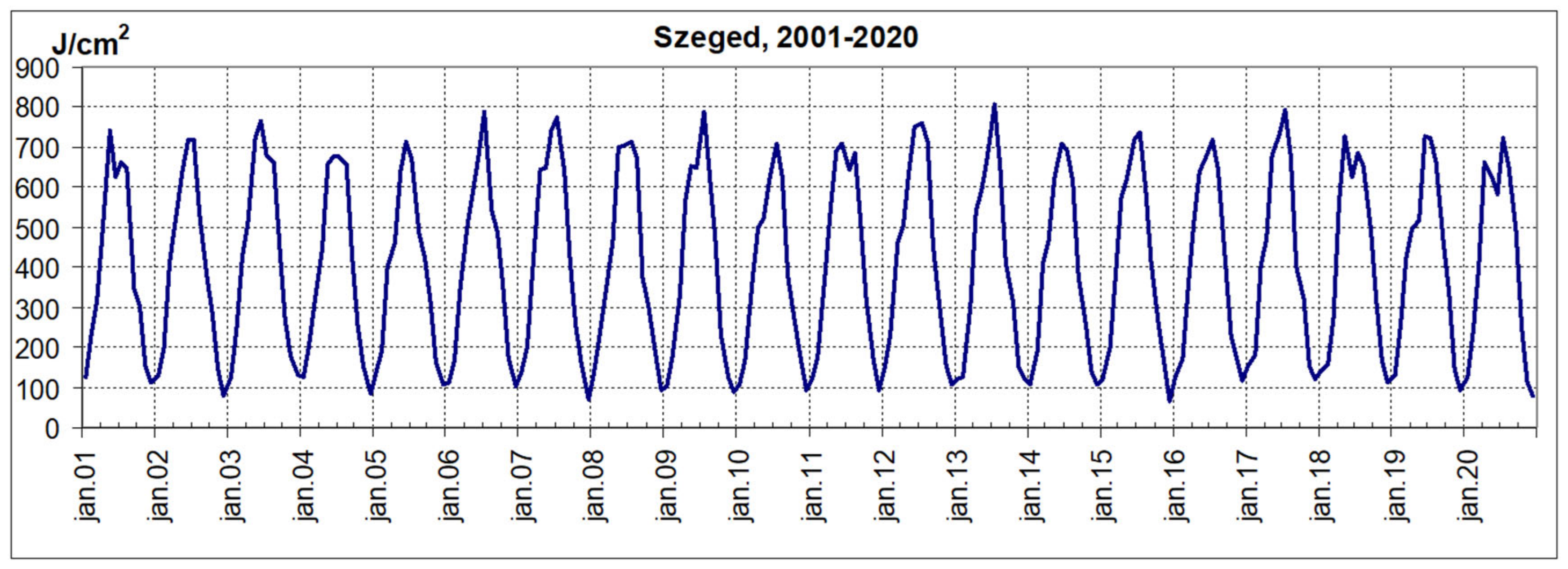
Figure 2 shows the time series of the monthly amounts. The annual runs seemed to fit very well together, probably due to homogenization. The monthly amounts ranged from about 100 to 800 J/cm
2 and their seasonal variation was marked. Therefore, in addition to the entire database, it was reasonable to perform the estimation for the summer and winter subsets and to analyze the results from a climatological point of view.
From a user, operational point of view, it was probably not significant to make early or late estimates. In the former case, we obtained unusually large errors and in the latter we obtained the same small errors. The results for the middle third of the month (i.e., day 10 to day 20) may have been relevant to the goal, so we will pay more attention to them below.
5.1. Peculiarities of the Monthly Course of the Average Relative Sliding Sum
The most important step in preparing the estimate was to generate the relative sliding sums (RSi,j) from the sliding sums and then analyze them statistically. Determining the mean ([RSi]) and median of RSi,j for the whole period, the summer and winter half-years, we saw that these could be assumed to be equal every day of the month (i) with a very good approximation. The winter half-year values of the mode differed significantly from the values of the whole period and the summer half-year.
The mean and median values followed an almost functionally increasing linear monthly course. The slope of the trend lines was between 0.032 and 0.033 in all six cases. The latter was also true for the modes, with the slope of the most variable monthly course being exactly 0.033. With a good approximation, this value could be taken as the average daily increase in the three characteristics.
The trend analysis performed for the middle third of the months (days 10–20) showed a slight difference from the previous ones due to the smaller number of items. The slope of the median and mode winter half-year trend lines was outside the range of 0.032–0.033, with 0.0311 and 0.0289, respectively.
Figure 3 shows the time course of the [
RSi] averages over the above period. The value of all three parameters on the 16th day of the month already exceeded 0.5, which means that half of the monthly amount was displayed around the 15th on average., and on 20th day, about two-thirds. The figure also shows that in the winter half-year, 4% more of the monthly amount was displayed on average every day of the period than in the summer half-year.
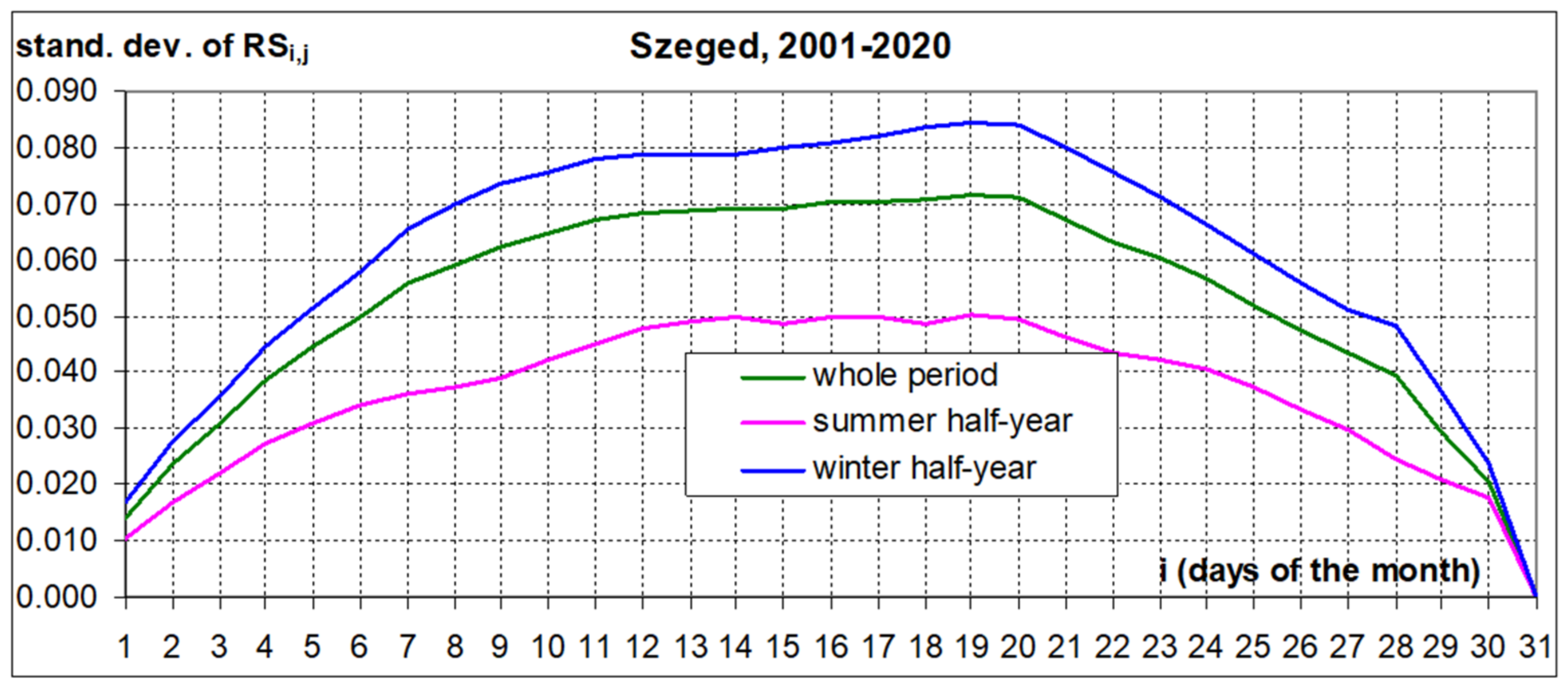
Figure 4 shows the monthly course of the standard deviation of the relative sliding sums (
RSi,j). The daily values of the standard deviation, except for the 31st day, were the highest in the winter half-year and the lowest in the summer half-year, and the values for the whole period were between the two. Their monthly averages were 0.061, 0.036 and 0.052, respectively. Among the curves describing this monthly course, only the one for the whole period showed a perceptible maximum on the 19th–20th. The difference between these values was greatest for the winter half-year and the summer half-year, 0.034 J/cm
2. The daily variation in the standard deviation between days 10 and 20 over the whole period and the winter half-year could be approximated very well, and in the summer half-year it could be reasonably approximated by a straight line with a slight slope.
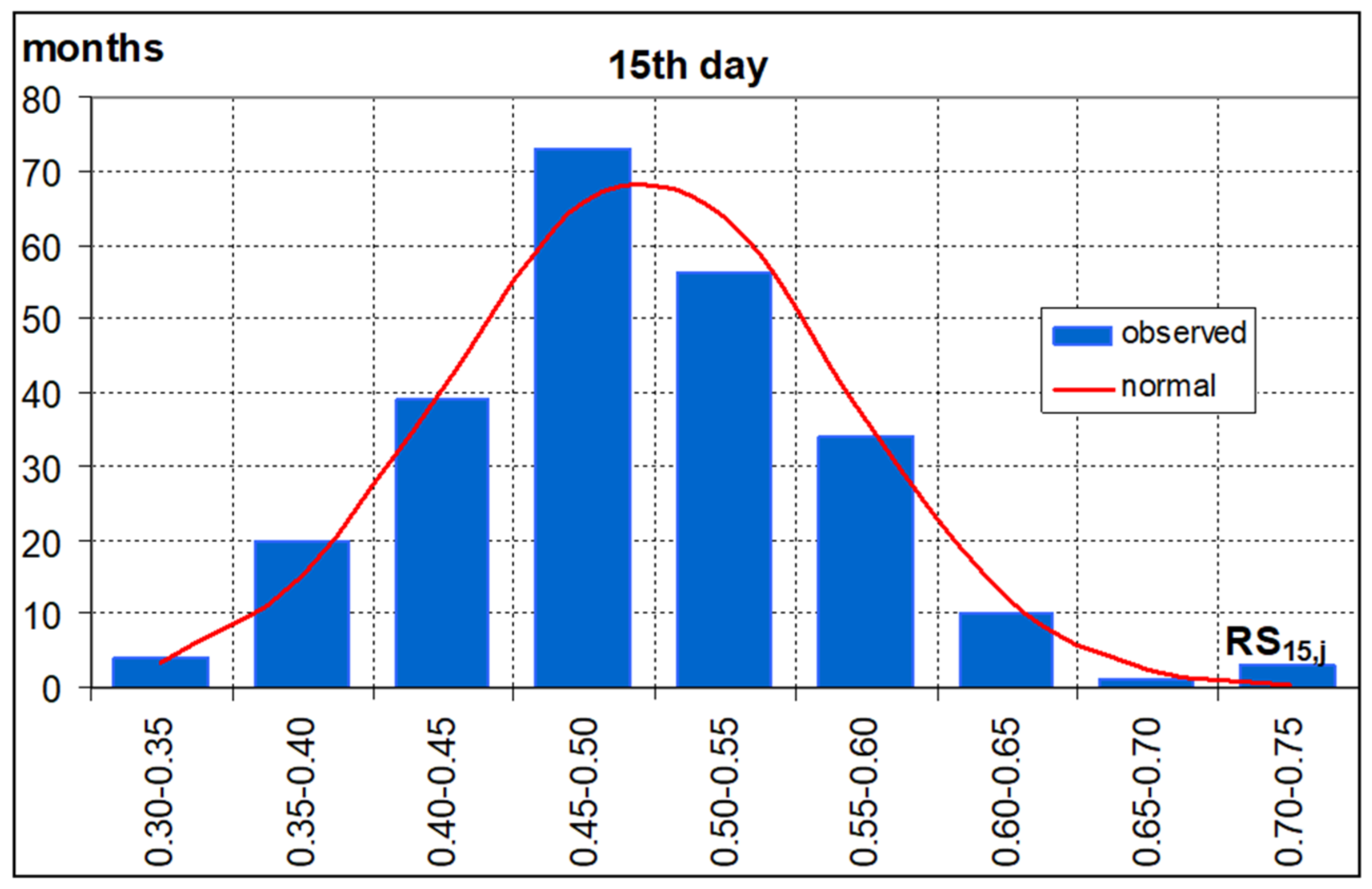
The good agreement between the three statistics—mean, median and mode—also shows that the daily values of
RSi,j were likely to be well-approximated by the normal distribution. Performing this approximation for the selected 10 days, we obtained that, with the exception of days 10, 11 and 18, the frequency distribution of
RSi,j could be approximated to the normal distribution at the 0.05 significance level.
Figure 5 shows the frequency distribution of
RSi,j observed and approximated by the normal distribution on the 15th day of the months (whole period). That is, how many of all the (240)
RS15,j values fall within the given interval.
5.2. Estimation, Estimation Error
Knowing the sliding sums Si,j and the average relative sliding sums [RSi], the estimation (11) could be performed. By doing this on the model development database, we actually performed the verification of the model, since by knowing the monthly amount to be estimated, the error of the model could be determined for each estimating time, only now for the days (i) of the month.
The errors were measured by three parameters:
|Ei|: the average of the absolute deviations defined in (6) calculated for the days of the month,
[Ei]: the relative error, which is the form of Equation (6) without absolute value, with the same mean,
RMSE (or RMSD, residual standard deviation): the square root of the mean of the squared differences.
However, the latter parameter, unlike the former ones, has a unit of measure (now J/cm
2). In our case, it can be calculated as follows:
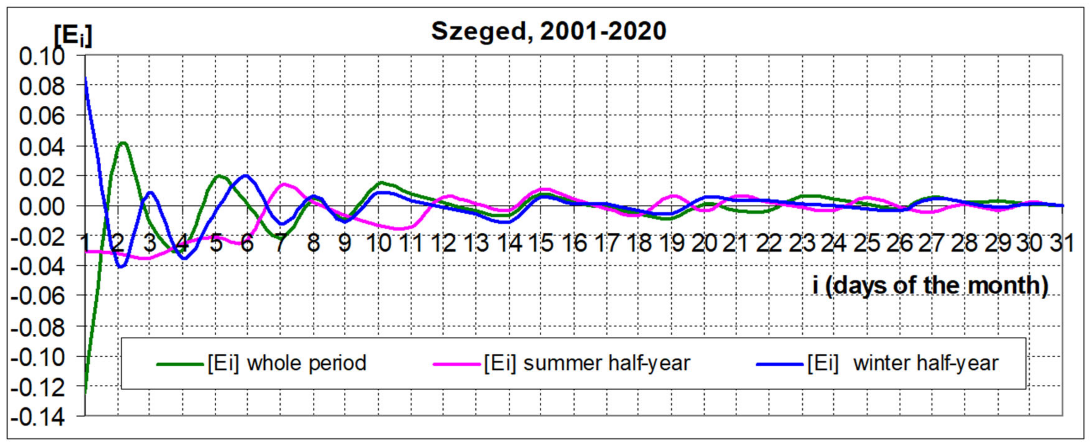
Figure 6 shows the monthly course of the mean relative error ([
Ei]) over the three study periods. You can see that this error parameter went down after the first few days of the month. It deviated increasingly from 0 with no detectable trend. However, by examining the sign of the relative errors per day, we could determine the number and proportion of underestimations and overestimations. We considered an underestimation to be if the estimated value was less than the one to be estimated, that is, in our case, if the numerator without an absolute value in Equation (6) was negative.
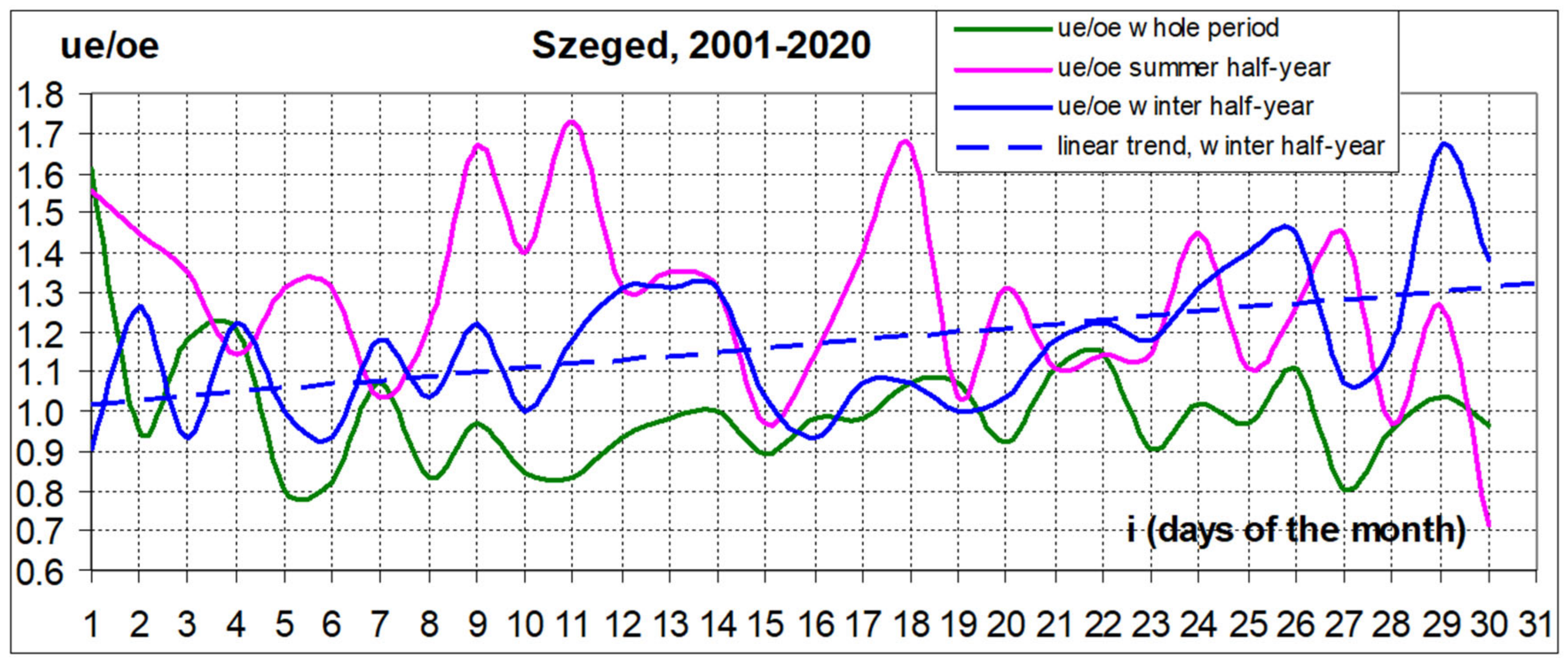
The monthly course of the ratio of the underestimation and overestimation (ue/oe) is shown in
Figure 7 over the three periods. The figure shows the predominance of overestimations (ue/oe < 1) over the whole period, with a higher number in the first half of the month. Seasonally, however, this rate fell sharply in favor of overestimations, with a frequency of 90% in the summer and 77% in winter. The periodical averages of the ue/oe ratio were similar: 1.00 for the whole period, 1.28 for the summer semester and 1.17 for the winter semester. The averages for the 10 days selected did not differ significantly from these: 0.96, 1.33 and 1.11, respectively. An appreciable linear trend could be observed only in the winter semester in the ue/oe ratio. The slope of the trend was positive, 0.01, i.e., the ue/oe ratio increased by an average of 1% per day during the month, indicating an increase in the number of underestimations.
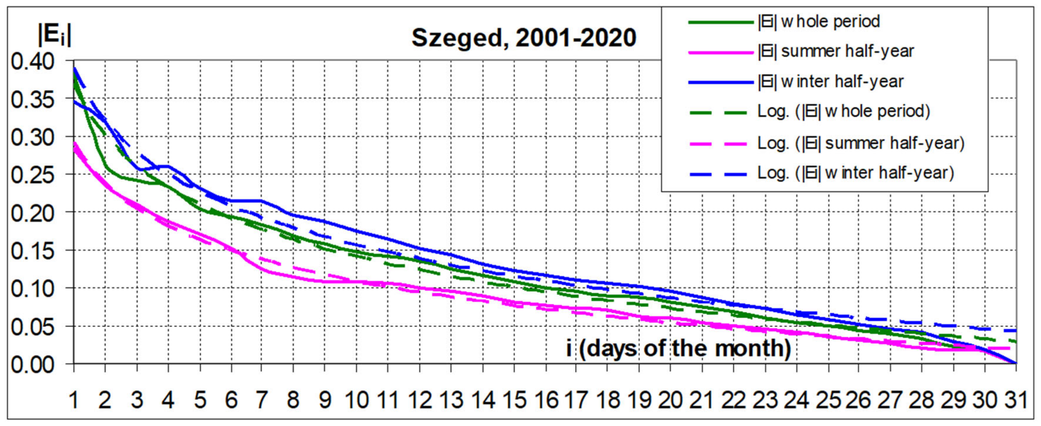
Figure 8 shows the averages of the absolute deviations |
Ei| at the estimated time points (as a percentage 100|
Ei|). We see a marked monthly runs in all three periods, which was very close to the logarithmic trend. According to the correlation index (that measured this connection), the degree of approximation was the best in the summer semester, followed by the whole period and then the winter semester.
Suppose we already accept the estimate at an average error of 20%. This error limit was already crossed by the curve on the 4th day in the summer semester, while only on the 8th day in the winter semester and on the 6th day in the whole period. At a 10% margin of error, these days were the 12th, 20th and 17th, respectively. The average values of |Ei| were also in the above order: 0.092, 0.135 and 0.120. These numbers also showed that we obtained a better estimate on summer days if we used the average relative sliding amount ([RSi]) corresponding to the semester. In the winter semester, however, we could estimate with a slightly smaller error if we used [RSi] for the entire period.
At 10 days in the middle third of the month, the curves in
Figure 7 were very close to a straight line. The slope of the lines gives the average decrease in error |
Ei| per day in this interval. This was 0.0051% in the summer semester (around 11% to 6%), 0.78% in the winter semester (17–10%) and 0.69% for the whole period (15–8%) (see below).
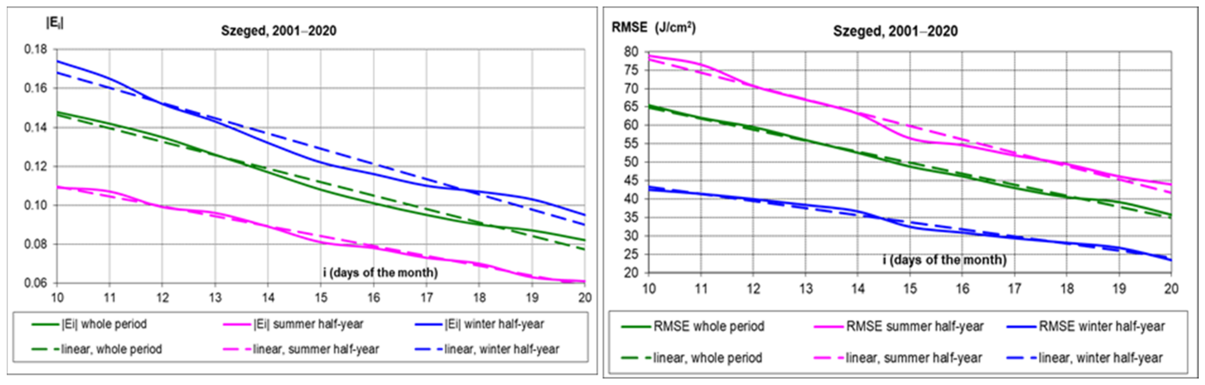
Figure 9 shows the values of the RMSE parameter (J/cm
2, see Equation (12)) at the estimated time points. We still saw a marked monthly trend in all three periods, which were also very close to the y = a · ln(x) + b logarithmic trend. The degree of approximation was still the best in the summer semester, followed by the whole period and then the winter semester.
The error thresholds were now the period averages of the parameter (J/cm2): 52.8 for the whole period, 64.6 for the summer semester and 34.2 for the winter semester. Consider a good estimate that is less than these averages. Examining the figure, we found that this now occurred in the full period and in the summer semester from the 14th day and from the 15th day in the winter semester. That is, practically every three periods in the second half of the month. From the RMSE values, it could be stated that in the summer semester, we made an error 1.7–2.5 times, on average 1.8 times larger than in the winter semester.
At 10 days in the middle third of the month, the curves in
Figure 8 could also be approximated very well by a straight line. The slope of the lines gave the average daily decrease in the RMSE in this interval. This was 3.6 J/cm
2 in the summer semester (approx. 79–44), 3.0 J/cm
2 in the whole period (approx. 65–35) and 1.9 J/cm
2 in the winter semester (approx. 42–23).
Figure 10 shows the mean in the absolute deviations (|
Ei|) and the RMSE values and the corresponding trend lines in the middle third of the months.
6. Discussion
A sliding-average model was developed to estimate the average of a climatic element measured at equal intervals over a time interval from within the interval. We have presented the structure of this and its version, the sliding-sum model for estimating the end-of-interval sums.
The operation and application of the sliding-sum model were presented by estimating the amount of global radiation in Szeged per month from the daily data. The database consisted of homogenized daily sums for the years 2001–2020. The model was run for the entire period and its two subsets, the summer and winter semesters.
First, we analyzed the statistical characteristics of the most important parameter of the estimation process, the monthly course of the average relative sliding sum that can be determined from long-term observational data. The mean, median and mode values followed almost the same increasing linear monthly trend over all three periods. The straight slope of the common trend could be taken as 0.033, so with a good approximation, this value gave the average daily increase in the three characteristics.
The trend analysis performed for the middle third of the months (days 10–20), i.e., for the period relevant for a good estimate, differed somewhat from the previous ones due to the smaller number of items. There was a greater difference between the slopes determined for the three periods.
The monthly course of the standard deviation of the relative sliding sums was described by curves with a maximum, with a more marked maximum only on the 19th and 20th day of the whole period and the winter semester.
A good match between the mean, median and mode also indicated that the daily values of the relative sliding sum were likely to be well approximated by the normal distribution. Performing this approximation for the selected 10 days, we obtained that, with the exception of days 10, 11 and 18, the frequency distribution could be approximated at the 0.05 significance level with the normal distribution.
Knowing the average relative sliding sums and the sliding sums, we performed the estimation on the model development database, i.e., the verification of the model. This is because by knowing the monthly amount to be estimated, the error of the model can be determined for each estimating time, i.e., for the days of the month. The calculated error parameters were the signed relative error, the absolute value of the relative error (absolute deviation) and the RMSE defined as the square root of the mean of the square errors.
There was no trend in the monthly course of the average relative errors per day, decreasing from 0 to a decreasing extent. However, examining the sign of these, we could determine the number and proportion of underestimations and overestimations. This ratio showed marked differences in the two semesters compared to the full period. An appreciable linear trend could only be observed in the winter semester in the middle third of the month.
In the daily averages of the absolute differences, we saw a marked monthly trend in all three periods, which was very close to the logarithmic trend for the whole month and the linear trend for the middle third of the months. The trend parameters could be used to determine the days on which the absolute deviation fell below a specified value.
The values of the RMSE parameter calculated at the estimated time points were also marked by a marked monthly trend in all three periods, which were also very close to the logarithmic trend for the whole month. The degree of approximation was still the best in the summer semester, followed by the whole period and then the winter semester. The RMSE values below the monthly average occurred in the second half of the month in all three periods. In the 10 days in the middle third of the months, these errors were also very well approximated by a straight line, the slope of which gave the average daily decrease in the RMSE in this interval. The decline was greatest in the summer semester.
7. Conclusions
The question is, of course, what is the result of the estimation for the database not involved in the model development? So, we split our database into a 15-year and a 5-year subset. Thus, our goal was to perform an estimation using the average relative sliding sums generated from the first subset and the sliding sums of the second subset to obtain an answer to this question. However, the average relative sliding sums produced in this way were almost exactly the same as those produced from the 20-year data. That is, the two types of estimation gave the same result. The reason for this is probably to be found in the special properties of the homogenized database.
A statistical approach to climate change requires a spatially and temporally representative database. However, the measurements, i.e., our raw climatological data series, are burdened with inhomogeneity due to the change in the measuring devices, the change in the location of meteorological stations and methodological changes. Our data series must therefore be homogenized, which means that we adapt the past measurements to the current measurement conditions [
34]. The MASH (Multiple Analysis of Series of Homogenization) software was developed in OMSZ for the complex handling of this problem [
35,
36].
However, it is quite certain that if we had used the original measured global radiation data, the results of the model would not have been so reassuring. Thus, the operative application of the model to promote solar energy utilization requires long-term measurements that are continuously corrected to the extent necessary, but that preserve local and seasonal properties.
So, the question is: should we use homogenized or raw (observed) data series for statistical analyzes? Izsáki et al. (2021) [
34] answer this question clearly: we can estimate climate change more accurately from homogenized data sets. We will formulate our answer to the SLIDSUM model after applying it to the estimation of monthly precipitation amounts. This is when we will run the model on the raw and homogenized data.


