Article

Diurnal Valley Winds in a Deep Alpine Valley: Model Results

by
Juerg Schmidli
1,2,* and
Julian Quimbayo-Duarte
1,2,3
1
Institute for Atmospheric and Environmental Sciences, Goethe University Frankfurt, 60438 Frankfurt am Main, Germany
2
Hans Ertel Centre for Weather Research, Goethe University Frankfurt, 60438 Frankfurt am Main, Germany
3
Grupo de Investigación de Calidad del Aire (GICA), Universidad Nacional de Colombia, Bogotá 111071, Colombia
*
Author to whom correspondence should be addressed.
Meteorology 2023, 2(1), 87-106; https://doi.org/10.3390/meteorology2010007
Submission received: 18 November 2022 / Revised: 15 January 2023 / Accepted: 2 February 2023 / Published: 14 February 2023

Abstract

:
Thermally driven local winds are ubiquitous in deep Alpine valleys during fair weather conditions resulting in a unique wind climatology for any given valley. The accurate forecasting of these local wind systems is challenging, as they are the result of complex and multi-scale interactions. Even more so, if the aim is an accurate forecast of the winds from the near-surface to the free atmosphere, which can be considered a prerequisite for the accurate prediction of mountain weather. This study combines the evaluation of the simulated surface winds in several Alpine valleys with a more detailed evaluation of the wind evolution for a particular location in the Swiss Rhone valley, at the town of Sion during the month of September 2016. Four numerical simulations using the COSMO model are evaluated, two using a grid spacing of 1.1 km and two with a grid spacing of 550 m. For each resolution, one simulation is initialised with the soil moisture from the COSMO analysis and one with an increased soil moisture (+30%). In a first part, a comparison with observations from the operational measurement network of MeteoSwiss is used to evaluate the model performance, while, in a second part, data from a wind profiler stationed at Sion airport is used for a more detailed evaluation of the valley atmosphere near the town of Sion. The analysis focuses on 18 valley wind days observed in the Sion region in September 2016. Only the combination of an increased soil moisture and a finer grid spacing resulted in a significant improvement of the simulated flow patterns in the Sion region. This includes a stronger and more homogeneous along-valley wind in the Wallis and a more realistic cross-valley wind and temperature profile near the town of Sion. It is shown that the remaining differences between the observed and simulated near-surface wind are likely due to very local topographic features. Small-scale hills, not resolved on even the finer model grid, result in a constriction of the valley cross section and an acceleration of the observed low-level up-valley wind in the region of Sion.

1. Introduction

Mountains cover a significant share of the Earth’s surface and have a major impact on the atmosphere. They can modify the synoptic-scale flow and influence the boundary-layer processes and turbulence [1]. Among mountain-induced flows, under fair weather conditions, thermally driven slope- and valley winds are key to local weather development and climate [2]. These wind systems have a direct impact on processes such as cloud formation, atmospheric trace species distribution and heat/moist exchange processes between the atmospheric boundary layer and the free atmosphere [3,4,5,6]. Both slope and valley winds are characterised by a reversal of flow direction twice a day, with transition periods from nighttime downwinds to daytime upwinds in the morning and vice versa in the afternoon, which normally occur after sunrise and sunset, respectively [7].
Thermally driven along-valley winds are usually the most dominant feature, as they tend to be stronger than the smaller scale flows developing on the slopes. Urban areas in mountainous terrain are typically located at the valley floor, implying that most of the meteorological measurements are made near these areas as well. The latter translates into a good record of observations of thermally forced winds on the valley floor, which means that the winds along the valley are not only the most dominant thermally forced flow, but also the best observed. The present study focuses on evaluating the skill of the Consortium for Small-scale Modelling (COSMO) model to simulate thermally induced local valley winds in the Swiss Alps during September 2016. The model setup used is configured to be close to the current operational setup used at MeteoSwiss.
In previous work, Schmidli et al. [8] evaluated the performance of the COSMO model in simulating the diurnal valley wind system over the entire Swiss Alps using a convection resolving setup. The authors observed a significant dependence of the results on the grid spacing (from 2.2 km, to 1.1 km), where the simulations with the coarsest grid spacing did not adequately reproduce the valley wind system, whereas the problem was partially solved by increasing the horizontal resolution. The latter is true for most large valleys (valley floor width ca. 2 km; the Rhine and the Rhone valleys, for instance) and medium-sized valleys (valley floor width ca. 1 km), while for small-sized valleys (valley floor width ca. 500 m; the Maggia valley, for instance) the wind speed amplitude signal is significantly underestimated, even for the simulation with finer grid spacing. An exception to the above finding was the poor performance of the COSMO model in simulating the valley wind in Sion, despite the station being located in a large valley. The strength of the up-valley wind was substantially underestimated in all model configurations.
Although fine grid spacing has proven to be helpful in the representation of the valley wind system, other factors such as the representation of orographic features, surface characteristics, land-atmosphere exchanges, soil moisture and turbulence closure appear to be important as well in the representation of the near surface atmosphere [9]. Liu et al. [10] highlighted that the quality of the underlying topography dataset used in the model proved to be one of the most critical factors in obtaining a successful fine-scale wind simulation when using high-resolution grid spacing. It is worth noting that the increase in the horizontal grid spacing needs to be supported by accurate surface characteristics in the numerical domain [10,11] and the state of the land surface [8].
Due to the complexity of the development of the thermally driven winds in complex terrain (such as the Swiss Alps), a better understanding of the local winds based on observations can be useful to improve the accuracy of the forecasts. Schmid et al. [12] studied the diurnal evolution of the three-dimensional mean wind structure in the deep Rhone valley near the town of Sion (where the COSMO model evidenced problems, as mentioned above). The authors used data from a radar wind profiler and a surface weather station recording continuously for a period of close to one year to study the atmospheric dynamics near the town of Sion. A subset of the data was selected to identify days with fair weather conditions to better characterize the thermally driven valley wind system at such a location. Results indicated a diurnal pattern that significantly changes throughout the year. During the warm season, a complex interaction of along- and cross-valley flow is observed including a relatively frequent occurrence of a layer of cross-valley flow, interlayered between low-level and upper-level along-valley flows. This layer typically extended from about 500 m above ground level (AGL) to about 1.5–2 km AGL.
In the present work, in light of the results presented in Schmidli et al. [8], a particular interest is devoted to the development of the diurnal valley wind system throughout the depth of the valley atmosphere at Sion, where the model previously evidenced problems, and the valley wind system was extensively studied by Schmid et al. [12]. We performed a set of sensitivity experiments to investigate the origin of the poor performance in the region of Sion, in which we increased the horizontal grid spacing, tested changes in the parameterization of surface-atmosphere exchange, turbulence, and shallow convection, and changed the initial soil moisture.
The remainder of the paper is organised as follows: the model description, experiments and observations are introduced in Section 2. The results from the numerical simulations are presented and discussed in Section 3. The conclusions are drawn in Section 4.

2. Methods and Data

2.1. Model Description

The model used in the present work is the non-hydrostatic Consortium for Small-Scale Modeling Model (COSMO), an area limited forecasting and climate prediction system at the mesoscale [13]. The model solves the governing thermo-hydrodynamic equations of the atmosphere using a split-explicit third-order Runge–Kutta time integration scheme [14,15]. In the present work, the numerical simulations are performed using COSMO version 5.7. We implemented a setup close to the operational configuration of Meteoswiss in 2021. Key differences include the use of a smaller domain in order to enable the use of the same domain for the 550 m simulations and a weaker smoothing of the model orography by using a cutoff filter at 3.5 Δ x instead of at 5 Δ x and an increased time off centering in the vertically implicit treatment of sound waves to increase the numerical stability of the model (betasw = 0.8 instead of the default value of betasw = 0.4). A further important factor for numerical stability and more accurate simulations is the use of the new cold pool filter (l_diff_cold_pools_uv = T) which is used to remove spurious cold pools which may form in complex terrain (this option is also used in the operational setup at MeteoSwiss).
The physical parametrizations implemented to account for subgrid-scale processes include a single-moment bulk cloud microphysics scheme [16], a radiative transfer scheme based on the δ -two-stream approach [17], and turbulent kinetic energy-based surface transfer and planetary boundary layer parameterization [18,19]. An extensive description of the model setup for convection-resolving simulations is presented in [20].
The reference simulation uses an integration domain covering the western and central part of the European Alps (see Figure 1a). The domain is smaller than the one used in [8], in order to enable the use of the same domain in the 500 m simulation. The vertical coordinate is discretised using 81 stretched levels on a Gal-Chen hybrid coordinate. The first mass point is located at 10 m above ground level (AGL). The vertical resolution increases from 20 m at the surface to 100 m at about 1000 m AGL (20 model levels in the first 1000 m AGL). The model top is set to 20 km above the mean sea level (MSL). A Rayleigh damping layer is applied to the upper part of the domain starting at 11 km.
The multi-layer soil model TERRA-ML [21] is used to parametrize the land-surface processes. The soil model is run using 10 soil layers with a total depth of 15.24 m. The soil layer thickness ranges from 1 cm to 7.48 m. The initial conditions for the soil temperature and the moisture content are derived from the COSMO-1 analysis obtained from MeteoSwiss. This dramatically decreases spin-up effects in the soil. The surface roughness length in COSMO is directly derived from the land cover data base. A parametrization of surface drag due to subgrid scale orography is not included.

2.2. Numerical Experiments
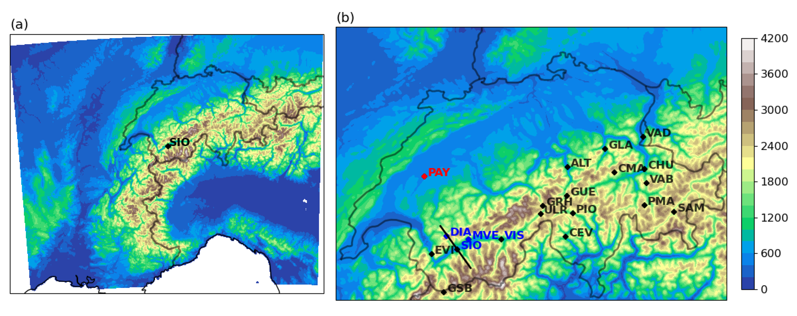
The analysis is carried out for 30 days in September 2016, of which 18 days were classified as fair-weather days, or valley wind days, following the criteria proposed by Schmid et al. [12]. These days are characterised by a clear signal of the thermally driven valley wind system. This classification is based on data collected at Sion station. All simulations are run from 00:00 UTC on 30 August 2016 to 00:00 UTC on 1 October 2016 (local time is equal to UTC +2), thus implying a two-day spin-up. Initial and hourly boundary conditions for the atmospheric and soil fields are provided by the COSMO-1 analysis (1.1 km horizontal resolution). In the remainder of the paper, all times mentioned correspond to UTC.
In order to investigate the poor skill of the reference simulation in the Sion region, many sensitivity experiments were carried out (see Appendix B). In this study, we report only on the four main simulations listed in Table 1, as these represent the most important sensitivities found, namely the sensitivity to the horizontal grid spacing and to the soil moisture initialization. In choosing an initial soil moisture anomaly of +30%, we follow the study of [22].

2.3. Observations

Standard hourly near-surface observations of the MeteoSwiss automatic monitoring network (SwissMetNet) of 2 m temperature, 2 m humidity, 10 m winds, surface pressure, and short wave incoming radiation are used. From all SwissMetNet stations, only 17 stations (see Figure 1b) showed a pronounced diurnal cycle in the wind speed. These stations are called diurnal wind stations from now on. We used the criterion used in [8] to define the diurnal wind stations within the domain.
The hourly wind values correspond to ten-minute averages based on vector averaged instantaneous measurements taken every second at the stations. The 10-min averages are calculated for the time interval HH:30.1 to HH:40.0, where HH refers to the corresponding hour. Similarly, the mean diurnal cycle of the wind speed and the wind direction, both in the observations and in the simulations, is calculated by vector averaging the hourly wind vectors and then converting back to mean wind speed and mean wind direction.
A Vaisala LAP3000 1290 MHz radar wind profiler was deployed at Sion airport (46.21864º N, 7.330215º E) at 482 m MSL. The instrument was operated using two different modes. A first low-mode configuration that covered an altitude range between 590 m MSL (corresponding to 108 m AGL) to 3714 m MSL with 58 m vertical grid spacing. A second high-mode configuration from 797 m (315 m AGL) to 8606 m MSL with a grid spacing of 144 m. A more detailed description of the operation of the instrument for this experiment can be found in [12]. Finally, data from radiosonde ascents (every 12 h, 00:00 and 12:00) at Payerne are also used.
For each model resolution, the model grid points associated with the individual surface stations are determined by minimizing an optimal distance to the stations. The latter is defined as a weighted average of the horizontal and vertical distances, with a stronger weight given to the vertical distance [23].
As seen in Figure 1b, the Rhone valley is approximately oriented along a west-south-west to east-north-east axis in the region of Sion. It is surrounded by high mountains both towards the south and the north. The highest mountains surrounding the valley to the south rise up to above 4.5 km MSL, while the average height of the northern ridge line rises from about 2.6 km in the west to 3.8 km MSL in the east. In the region of Sion, the height of the northern ridge varies between 2.1 km and 3.2 km MSL (see Figure 1 in [12] for a picture of the topography and land cover in the region).

3. Results

The presentation of the results is divided into six subsections. First, an overview of the weather conditions in Switzerland during September 2016 is given, followed by a brief evaluation of the diurnal cycle of the valley wind for the valley wind stations in Switzerland. In Section 3.3, the evolution of the diurnal valley wind throughout the depth of the valley atmosphere in the region of Sion is documented using wind profiler data and compared to the model simulations. This very local perspective is complemented by a documentation of the mean diurnal cycle of the wind system in the entire Wallis region in Section 3.4. In Section 3.5, the similarities and differences in the simulated flow for two different cases are shown in more detail in order to shed light on the often poor performance of the reference simulation C1r in the Sion region. It is shown that the low skill of the reference simulation is, among other factors, linked to a poor representation of the thermal stratification in the valley which is evaluated in more detail in Section 3.6.

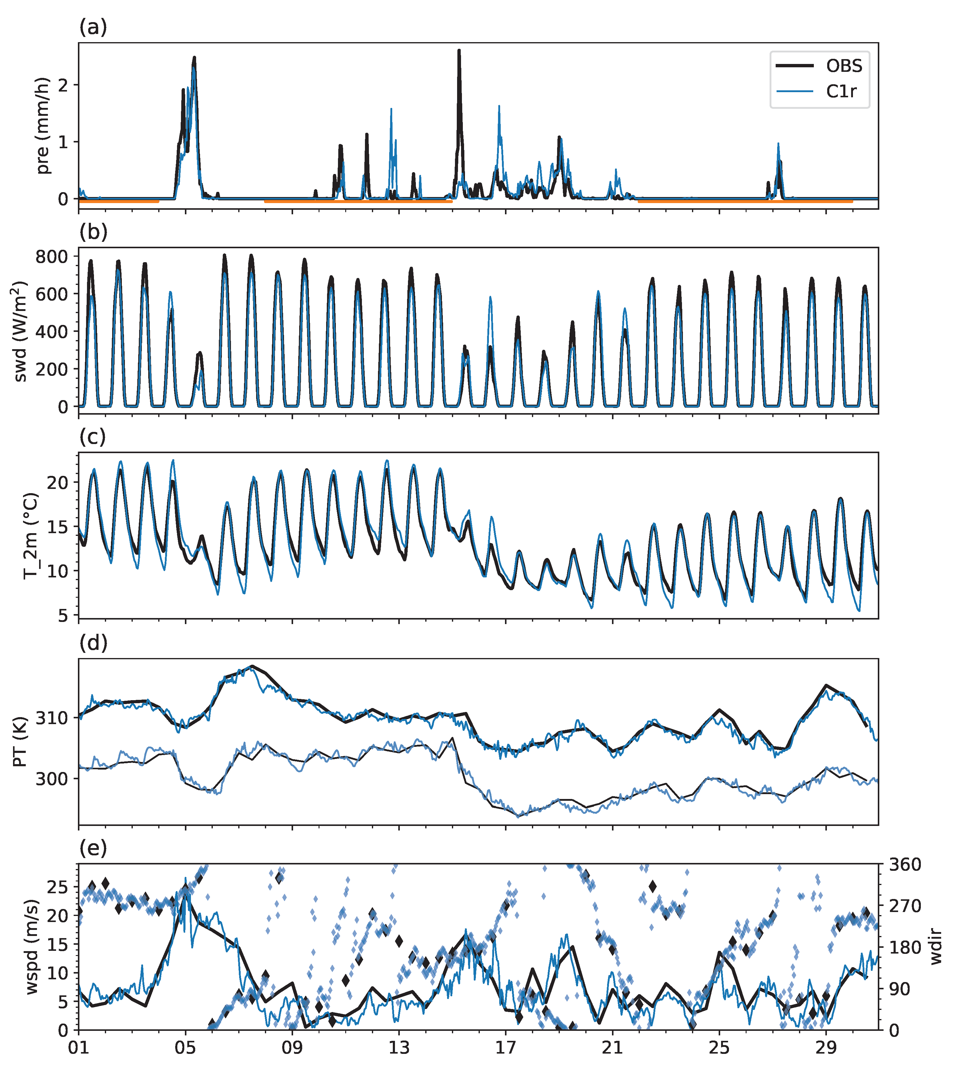
3.1. Overview of Weather Situation in September 2016

The observed weather in Switzerland during the analysis period in September 2016 is summarised in Figure 2. Time series of precipitation, global radiation, and 2 m-temperature during September 2016 for both observations and the C1r reference simulation are shown in the top three panels. The results displayed represent the average over all the valley-wind stations. With respect to climatology, the month of September 2016 was exceptionally warm with high solar irradiance (for the time of the year). In the first two weeks, a high-pressure system dominated the area, with the exception of the passage of a cold front on 4 September. At the end of the month, again, a high-pressure system dominated. Even if some convective precipitation was observed in some locations (but not in Sion) during the high-pressure dominated periods, daytime cloudiness remained low and global radiation high, enabling the development of distinct thermally driven wind systems during most of the month (see orange lines in Figure 2a).
A clear diurnal cycle of 2 m temperature is visible on most days, indicative of the strong global radiation and limited cloudiness (see Figure 2c). The month is characterised by a very warm first half, and a warm second half. The regular daily evolution is interrupted by the cold frontal passage on 4 September and the more disturbed conditions around 18 September. The reference simulation performed well in simulating the main weather features throughout the month, although the model exhibited a cold bias on several nights.
Figure 2d,e use data collected from the twice-daily radiosonde launches at Payerne to display time series of potential temperature at 2000 m AGL (thin lines) and 4000 m AGL (thick lines, see Figure 2d). The data from the radiosonde launches were also used to display wind speed (lines) and direction (diamonds) at 4000 m AGL (see Figure 2e). During the fair weather days, the wind speed barely reaches 5 m s 1 , while, at the time of the disturbance, it reached a magnitude as high as 20 m s 1 . It is worth noting the model’s accurate simulation of the upper-level evolution (see Figure 2d,e) in terms of the potential temperature (at both 2000 m AGL and 4000 m AGL) and wind magnitude; even the wind direction is well captured in the reference simulation. This corroborates that the free-tropospheric evolution stays close to the large-scale evolution in our hindcast setup forced by the “perfect” lateral boundary conditions from the COSMO-1 analysis.
We conclude this overview with a brief model evaluation of the two key simulations C1r and C500w in terms of the mean diurnal cycle (averaged over the valley wind days) of a selection of key near-surface variables, including incoming solar radiation at the surface (swd), the 2 m temperature, the 2 m dew point temperature, and the relative humidity, shown in Figure 3. It can be seen that the incoming solar radiation, averaged over the valley wind stations (top row), is underestimated by both simulations. Despite the identical solar forcing, the evolution of the near-surface thermodynamic fields differs significantly between the two simulations. The moisture evolution in terms of dew point temperature and relative humidity is much closer to the observations for the simulation with the increased initial soil moisture (C500w). In terms of the 2 m temperature, the reference run C1r exhibits a too low nighttime minimum, while C500w underestimates the daytime maximum temperature. Very similar results are found for the evolution at Sion (bottom row), with the exception of incoming solar radiation which is lower in C1r, possibly as the result of a negative soil moisture-cloud feedback, that is of drier soil leading to more clouds due to more vigorous thermals (e.g., [22]). The results for C1w lie between those for C1r and C500w (not shown). Overall, the C500w simulations are significantly closer to the observations, in particular for the moisture field.

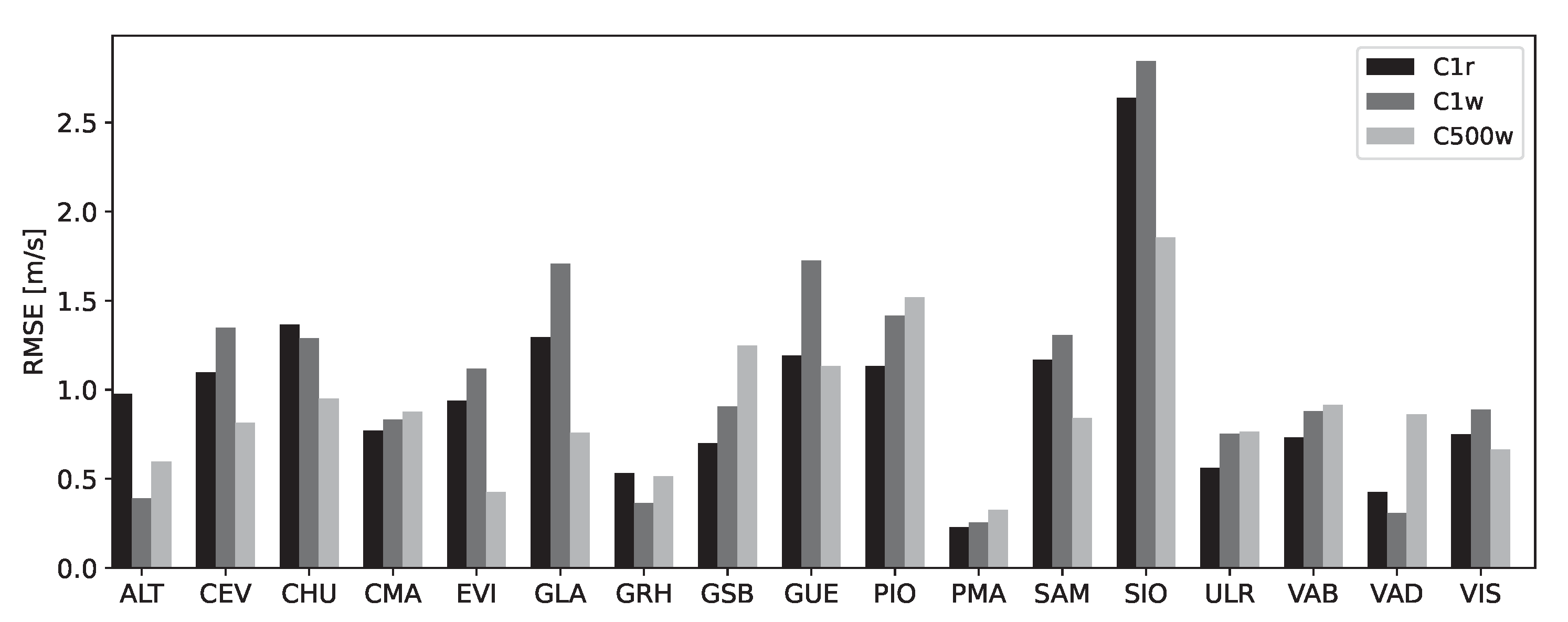
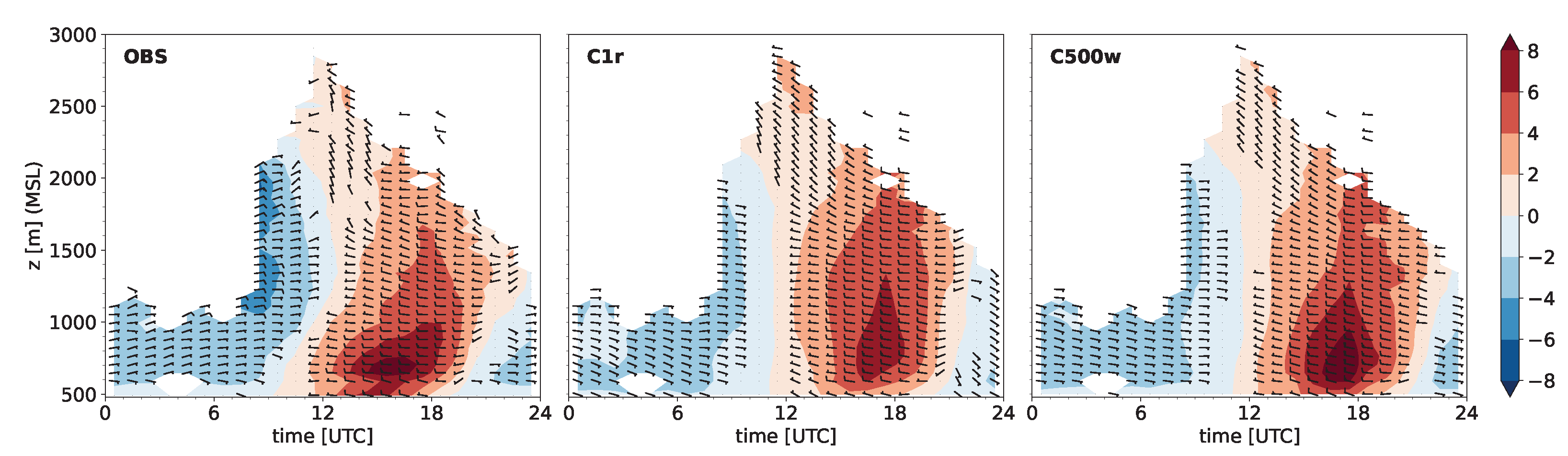
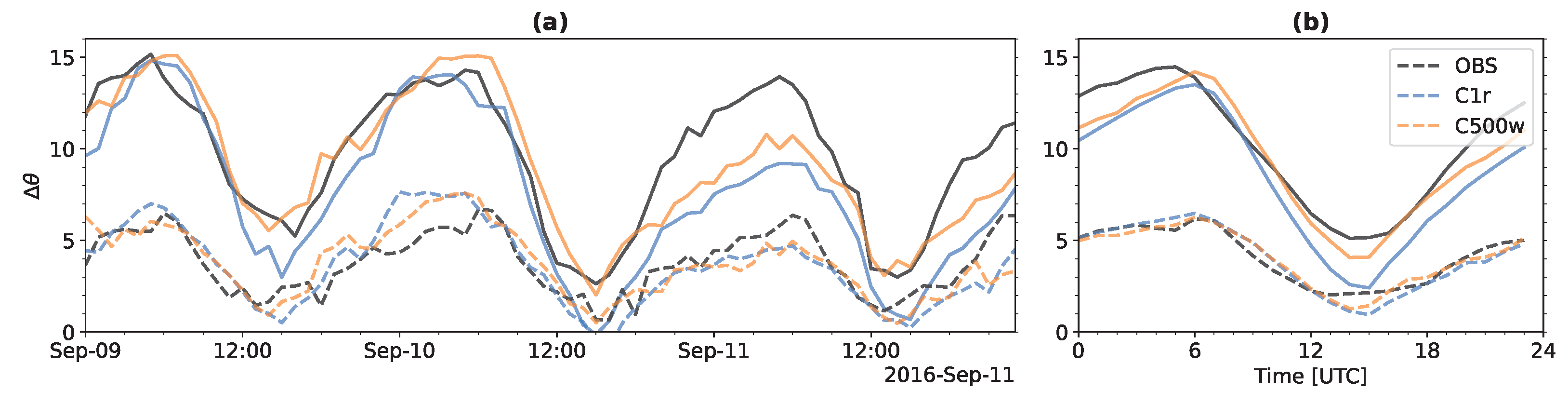
3.2. Brief Evaluation of the Diurnal Valley Winds

The 10 m wind speed, as simulated by the simulations C1r and C500w, is compared with observations in terms of the mean diurnal cycle in Figure 4 for two representative stations (Visp, Cevio) and Sion. Visp is representative for a station in a large valley, and Cevio for one in a small valley (see also [8]). Overall, at both Visp and Cevio, the C1r simulation performed well in reproducing the magnitude of the wind, although a small overestimation of the wind during the nighttime hours was detected at the large valley station of Visp. However, the largest error appears at Sion where the model cannot reproduce the wind magnitude by overestimating it through the night, and underestimating it during the day. The accurate simulation of the wind direction becomes a problem of the small valley station of Cevio, where only in the afternoon hours did the model results approach the observed wind direction. In the other two stations, the wind direction is well represented.
The representation of the mean up-valley wind for all valley wind stations is quantified in Figure 5 for the three main simulations. On average, the performance of C500r is similar to C500w, but the skill for Sion is even lower than for C1r, thus no results are shown for C500r. The RMSE of the reference simulation (C1r) for Sion is 2.7 m s 1 , which is double the magnitude or more than the error for the other stations. This is consistent with the findings of Schmidli et al. [8] based on an earlier model version and for a different period (July 2006).
The error appears to be caused by the poor representation of the local orography in C1r, due to the complexity of the terrain found in this area. This is evidenced by the decrease in RMSE for the simulation C500w, where apparently the finer horizontal grid spacing allows a better representation of the complex terrain. Note, however, the second important difference between C1r and C500w is the higher initial soil moisture (+30%) for C500w. Only the combination of both modifications leads to improved results. Increasing the initial soil moisture without increasing the grid spacing (simulation C1w), or increasing the grid spacing without increasing the initial soil moisture (simulation C500r, not shown) does not improve the model performance for Sion.
Overall, the effect of the higher resolution with the increase of the initial soil moisture is positive; for several stations, the error decreased (even by a factor of two, see Evionnaz station, EVI). However, in some cases (such as Vaduz, VAD), the error increased compared to C1r. It is worth noting that, for the high resolution simulation (C500w), the Sion station still shows a large error compared to the other stations, which requires further investigation.

3.3. The Valley Wind at Sion

Figure 6 shows the mean diurnal cycle of the valley wind (vector averaged) at Sion throughout the valley atmosphere for the valley wind days in September 2016 for observations and simulations. The observations are based on a combination of the low-mode wind profiler and weather station data. A typical diurnal pattern of daytime up-valley and nighttime down-valley flow can be clearly observed. During the night hours, the wind flows in the down-valley direction until about 09:30, 3.5 h after sunrise (around 06:00), when the morning transition of the valley wind begins. The transition from down-valley to up-valley flow occurs over a two-hour period with weak winds (wind speed less than 2 m s 1 ). The transition is first observed near the surface and then propagates vertically over a time frame of around three hours. More specifically, an along-valley wind speed above the 4 m s 1 threshold is first observed at the lowest three levels at about 11:30; 2.5 h later, it is observed at 1300 m MSL, and, another hour later, it reaches 1800 m MSL. This effect is also seen in the evening transition when the wind deceleration is first observed near the surface and propagated vertically afterwards. Note also the signature of a cross-valley flow above about 1700 m MSL in the time period from 12:00 to 15:00.
The C1r simulation is able to reproduce the main wind features throughout the day, although the flow is weaker and it cannot adequately represent the wind reversal during the morning and evening transition at Sion near the surface. The morning transition occurs almost simultaneously throughout the atmosphere in C1r. Actually, the maximum up-valley wind appears to propagate from mid-levels down to the valley floor. The evening transition compares reasonably well with the observations. The C500w simulation improves the reproduction of the wind at Sion during the valley wind days. The time-height evolution is significantly closer to the observed evolution. Note the slight delay in the onset of the up-valley wind with height and the stronger up-valley wind maximum. The latter can be better seen in the vertical profiles shown in Figure 7.
Figure 7a presents the vector-averaged vertical profiles of the mean down-valley wind at 08:00. The C500w simulation agrees well with the observations near the ground. However, above 800 m MSL, both C1r and C500w underestimate the magnitude of the wind speed. It is worth noting the good performance of both simulations in representing the wind direction at Sion, where a flow in the down-valley direction is clearly observed at this time. The corresponding plot for the mean up-valley wind is shown in Figure 7b. As before, C500w agrees better with the observations. In particular, the low-level jet magnitude is well represented and the overall vertical profile of wind speed and wind direction is closer to the observations than for C1r. Note also the good representation of the change in the mean wind direction above 1000 m MSL for C500w. This change in the mean wind direction in the layer extending from 1000 m to 1800 m MSL is likely the imprint of the relatively frequently observed cross-valley flow in that layer [12]. While C500w captures well the lower boundary of this layer, the layer seems to be too deep in the model.
An evaluation of the temporal variability of the wind is given in Figure 7c. It shows the bias and the mean absolute error (MAE) computed with respect to high-mode wind profiler. Note the improved performance in terms of both MAE and bias using the finer grid (C500w), especially near the surface and also the improved representation of the upper level wind direction (red dashed curve).
What makes the simulation of the near surface winds at Sion so difficult? While clear improvements have been obtained with C500w (see Figure 4, Figure 6 and Figure 7), the error of the simulated near surface wind is relatively large, compared to other valleys (see Figure 5). To address this question, Figure 8 shows the local terrain in the region of Sion in terms of the terrain height at different resolutions, and a 3D view of the region. It can be seen that the valley undergoes a constriction in the region of Sion and the location of the MeteoSwiss station Sion, located at Sion airport. There are three small-scale hills to the northwest of the airport: (1) The Crêtes des Maladaires with a height of 574 m MSL, (2) the Mont d’Orge with a height of 787 m MSL, and (3) the hill with the Château de la Soie with a height of 873 m MSL. These three hills reach about 90 m, 300 m, and 390 m above the height of the valley floor at the observation site. In particular, the first two constitute an obstacle to the along-valley flow. These small-scale hills are not represented in the model orography at either resolution. Nevertheless, the orography of the valley floor is better represented in C500w, and the minimum elevation is located in the correct region in contrast to C1r. We hypothesise that these small-scale hills lead to a local flow acceleration which can not be accurately represented with the currently used model resolutions.
In summary, the Sion region is challenging both at the mesoscale, i.e., interaction of along- and cross-valley flows, and at the very local scale (small-scale hills). For the former, the combination of increased soil moisture and going to 500 m grid spacing leads to a significant improvement, while, for actually representing the latter, an even higher resolution would be required.

3.4. The Wallis Valley Wind System

To complement the very local perspective, the mean diurnal cycle of the valley wind system in the entire Wallis is shown in Figure 9 for the valley wind days in September 2016 for both C1r (left column) and C500w (right column). The figure shows the mean wind speed and direction at 200 m AGL, which is the approximate height of the up-valley jet maxima at Sion. At the end of the night (04:00), C1r simulates a weak down-valley wind in the upper Wallis and a strong down-valley wind in the lower Wallis reaching the shore of lake Geneva. The C500w simulation, on the other hand, shows a weaker down-valley flow with a magnitude mostly below 3 m s 1 ; in addition, the stronger flow vanishes about 15 km before the lake shore.
At midday (12:00), the along-valley wind has reversed and a weak up-valley wind is visible in both simulations. Furthermore, there is a cross-ridge flow visible on the northern side of the valley. This cross-ridge flow is rather weak and restricted to the mountain passes in C500w, while it is stronger and more widespread in C1r. In the late afternoon (16:00), the up-valley flow in C500w is stronger and spatially more continuous. The C1r simulation reproduces a patchy up-valley wind due to (too) strong cross-valley flow, which seems to be unrealistic (see Section 3.5). Finally, during the evening transition, at 20:00, the C1r simulation exhibits an almost quiescent atmosphere at this level. The C500w simulation, on the other hand, still shows a light up-valley flow.

3.5. Valley Flow Patterns: Two Case Studies

Up to this stage, the focus has been mainly on the mean diurnal cycle of the valley wind during the valley wind days. Next, results for two specific cases are presented; one case where the reference simulation C1r performs relatively well (23 September 2016), and a second case where its performance in comparison to the observed surface winds at Sion is poor (10 September 2017). We investigate the flow patterns in the region and compare C1r with C1w and C500w to shed light on the cases of the poor performance of C1r on certain days.
On 23 September 2016, all three simulations exhibit a similar pattern of up-valley flow, which is confined to a more or less continuous ribbon following the valley geometry (see Figure 10, left column), the latter being somewhat narrower, stronger, and more continuous in C500w. The up-valley wind is strongest in the lower part of the valley atmosphere (see Figure 10, right column). It can be seen that the up-valley wind maximum is stronger in C500w, likely associated with the higher horizontal resolution and more stable stratification of the lower valley atmosphere in C500w. Winds coming from the small tributaries (cross-valley) near Sion can be observed in all three simulations (see Figure 10, left column), but they decrease in strength and extent going from C1r to C1w and from C1w to C500w. These gap flows are the result of cooler air from the Bernese Oberland (to the north) flowing into the warmer Wallis region, which is the typical location of the Alpine heat low. This regional upper-level temperature contrast can be clearly seen by means of the potential temperature contours in the vertical cross-sections. The cooler gap flows then transitions into (katabatic) downslope flows along the northern side of the valley (seen at about 20 km). Despite the differences, all three simulations agree reasonably well for this case in terms of the main features.
The flow patterns for the second case (10 September 2016) are shown in Figure 11. For this case, there are large differences between the three simulations. While the flow pattern of a well developed up-valley wind is simulated in C500w, similar to the first case (September 23), the reference simulation C1r shows a very different flow pattern. In C1r, strong cross-valley flows have interrupted the formation of the up-valley flow. While cross-valley flows from the tributaries can be observed in both simulations, only in C1r can these flows reach the valley floor and sweep across the entire valley cross section. In C500w, the stronger stratification of the lower valley atmosphere protects the up-valley flow, as the weaker cross-valley flow is restricted to upper levels. The flow pattern for the C1w simulation lies in between these two extremes. While the strength of the gap flows is weaker than in C1r, they are nevertheless strong enough to locally disrupt the formation of the up-valley flow, for example, to the east of Sion.
In order to further assess the simulations and obtain an idea of the true flow pattern in the valley at the location of Sion, the simulated wind evolution throughout the atmosphere is compared with observations in Figure 12. The basic features of the observed evolution are similar to the monthly average showed in Figure 6, a low-level up-valley jet during daytime, an upper-level maximum in the nighttime down-valley flow and wind reversals originating at the surface and propagating upwards. The evolution above about 1000 m MSL is, however, highly variable and indicative of the impact of the cross-valley flow. The cross-valley flow can be clearly seen above 2000 m MSL starting at 12:00 and down to 1000 m MSL at 16:00. While none of the simulations are perfect, C500w captures both the development of the strong low-level up-valley flow and of the cross-valley flow at higher levels. In particular, the former is poorly represented in the other two simulations.
For an easier quantitative assessment, we turn to vertical profiles of wind and potential temperature at 16:00 at Sion (see Figure 13). The observed wind profile clearly shows a jet-like structure with a maxima at 700 m MSL (220 m AGL). Within the jet region, the wind is in the along-valley direction. The wind speed reaches a minimum at 1000 m MSL and increases to a broad second maxima at 1600 m MSL. It can be clearly seen that the upper level maxima is related to the cross-valley flow and that the influence of the flow reaches down to 900 m MSL, just 400 m AGL. Abrupt changes in the observed wind direction with height suggest that the flow might be rather variable in time, and possibly also turbulent.
From the simulations, it can be seen that C1r fails to reproduce the strong up-valley flow, while C500w reproduces the jet-like structure of the up-valley wind (also in terms of the correct along-valley wind direction) and also the cross-valley flow layer (the non along-valley wind direction from 1300 m to 2800 m MSL). The model is not perfect, but the main features are represented well, confirming the usefulness of C500w for the investigation of the complex flow patterns in the Sion region and the deficiencies of C1r.
A comparison of the potential temperature and the specific humidity at Sion for the two simulations (see Figure 13b) shows that the valley atmosphere is almost neutrally stratified in C1r, while there are several layers with stable stratification in C500w, in particular below 1400 m MSL. Clearly, the poor representation of the temperature structure in the valley atmosphere in C1r is related to the poor representation of the flow patterns. Due to the too weak stratification of the valley atmosphere, the cross-valley flow can penetrate down to the valley floor and disturb the formation and evolution of the along-valley wind. While the temperature structure for C1w is close to that for C500w, the representation of the winds lies in between that for C1r and C500w, indicating the importance of the finer grid spacing for the skill of C500w (in addition to the change in initial soil moisture).
Unfortunately, no direct observation of the temperature and moisture structure in the valley is available. The stratification of the valley atmosphere in the region of Sion can be approximated by using data from nearby slope and mountain stations, see the next section, or we can compare it to the observed temperature and moisture structure from the radiosonde ascents at Payerne (which are only available at 00:00 and 12:00). The temperature and moisture structure at 12:00 averaged over the valley wind days is shown in Figure 13c. It can be seen that C500w compares well with observations, both in terms of temperature and moisture (except for a slight moist bias at upper levels), while C1r has a warm and dry bias in the lower atmosphere and a larger moist bias at upper levels, above 2500 m MSL. The vertical structure of the moisture bias in C1r could indicate too strong vertical mixing in the model.

3.6. Evaluation of Atmospheric Stratification

Time series of the valley stratification between 9 and 11 September are displayed in Figure 14 for the entire valley depth (solid lines) and the lower part (dashed lines). The observed bulk stratification over the full depth varies between a nighttime maximum of about 15 K and a daytime minimum of 3 K. While C500w represents the daytime minimum well, the stratification is too low in C1r on all three days and it even reaches 0 K on 10 September. In the lowest 1000 m AGL, the observed bulk stratification varies between a nighttime maximum of 6–7 K and a daytime minimum of 1–2 K. Both simulations tend to underestimate the daytime minimum, but the discrepancies are smaller for C500w, in particular for 10 September.
Figure 14b generalises the results to all valley wind days. It can be seen that, on average, both models tend to be too weakly stratified in the afternoon hours, although the discrepancy is larger and of longer duration for C1r.
The results highlight the importance of an accurate simulation of the thermal structure of the valley atmosphere. Only the combination of an increased initial soil moisture (+30%) and an increased horizontal resolution (550 m versus 1.1 km) resulted in an improved representation of the valley wind system in the Sion region. The moister soil leads to a better representation of the thermal structure of the valley atmosphere (for the period considered), while the finer horizontal grid spacing leads to a better representation of the local topography. Further evidence of a generally poor representation of the temperature structure of the atmosphere over Switzerland for the valley wind days in September 2016 in the C1r simulation and an improved representation in C500w is given in Appendix A.

4. Conclusions

This study combines the evaluation of the simulated surface winds in several Alpine valleys with a more detailed evaluation of the wind evolution for a particular location in the Swiss Rhone valley, at the town of Sion, during the month of September 2016. Four numerical simulations using the COSMO model are evaluated, two using a grid spacing of 1.1 km (C1r, C1w) and two with a grid spacing of 550 m (C500r, C500w). For each resolution, one simulation is initialised with the soil moisture from the COSMO-1 analysis (C1r, C500r) and one with an increased soil moisture (+30%; C1w, C500w). In the first part, a comparison with observations from the operational measurement network of MeteoSwiss is used to evaluate the model performance, while, in a second part, data from a wind profiler stationed at Sion airport are used for a more detailed evaluation of the valley atmosphere near the town of Sion. The analysis focuses on 18 valley wind days observed in the Sion area during the month of September 2016. The model evaluation leads us to the following conclusions:
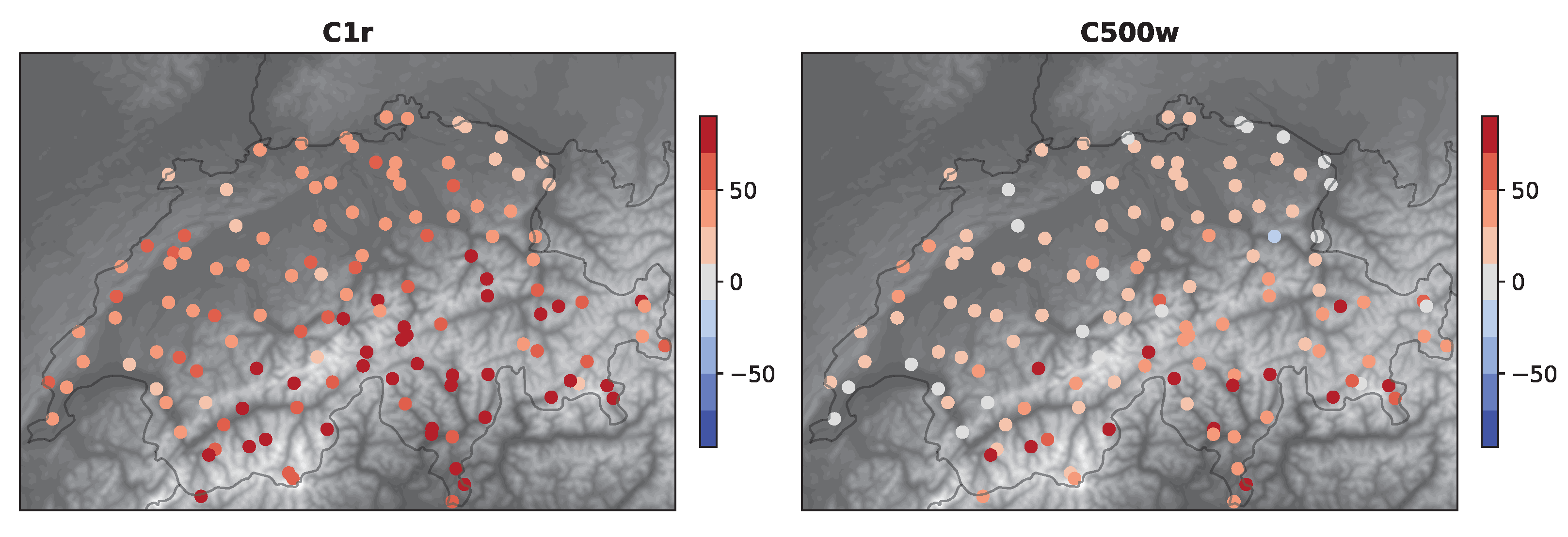
  • The general results are consistent with those a previous study evaluating the COSMO model performance in the Swiss Alps [8]. We find a generally good representation of the mean diurnal cycle of the valley wind in the larger Alpine valleys and still a rather low skill for the MeteoSwiss station located at Sion airport. The latter is the case, despite the use of an updated model version (COSMO version 5.7 versus version 5.0) and a different analysis period (September 2016 versus July 2006). Furthermore, it was shown that the reference simulation C1r and the simulation C500r have a dry bias, which is corrected by the sensitivity experiments with an increased soil moisture (C1w, C500w). After our study was completed, a deficiency in the COSMO soil model was discovered, which led to a dry bias in the COSMO-1 analysis in September 2016 and hence also in C1r and C500r. This deficiency has been corrected in the meantime;
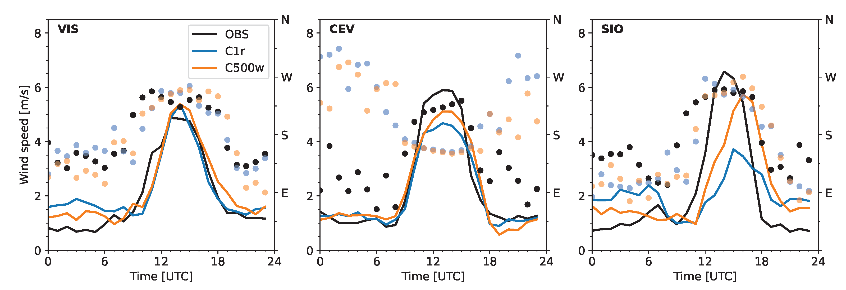
  • The wind profiler allowed for the documentation of the wind evolution throughout the valley atmosphere above Sion airport. A typical diurnal pattern of daytime up-valley and nighttime down-valley flow can be clearly observed in the lowest 1500 m AGL. During the nighttime, an elevated down-valley flow is observed which transitions around midday to a strong up-valley jet with maximum wind speeds at about 200 m AGL. Both the morning and the evening transitions start at the surface and propagate to higher elevations over a period of several hours. A special feature of the wind pattern above Sion is the frequent occurrence of an elevated layer of cross-valley flow, the imprint of which is also seen the the mean diurnal cycle. While both simulations (C1r and C500w) were able to represent the main features, the time-height evolution of the mean valley wind is closer to the observed evolution in C500w (better representation of the up-valley jet maximum, transition periods, and specific cases);
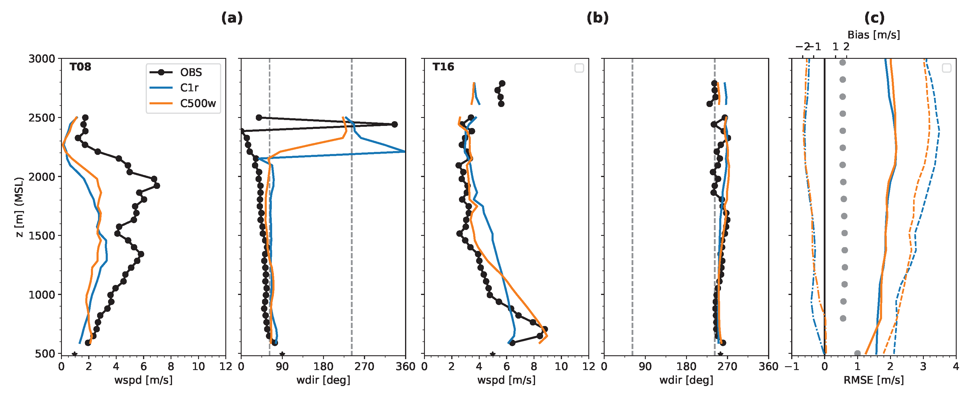
  • To shed light on the rather low skill of the reference simulation C1r, the diurnal evolution of the winds on two contrasting and representative days has been compared. On the first day, the difference between C1r, C1w, and C500w is rather small, while, on the second day, the flow patterns are very different. It has been shown that the particular poor performance on this day is linked to the simulation of a too strong cross-valley wind which interrupts the formation and evolution of the along-valley flow. In the reference simulation, this cross-valley wind can reach the valley floor, while in reality and in C500w, the cross-valley wind is restricted to higher levels and does not reach the valley floor. The flow pattern for C1w lies in between the two extremes, indicating that both the increased initial soil moisture and the finer grid spacing are important for the skill of C500w;
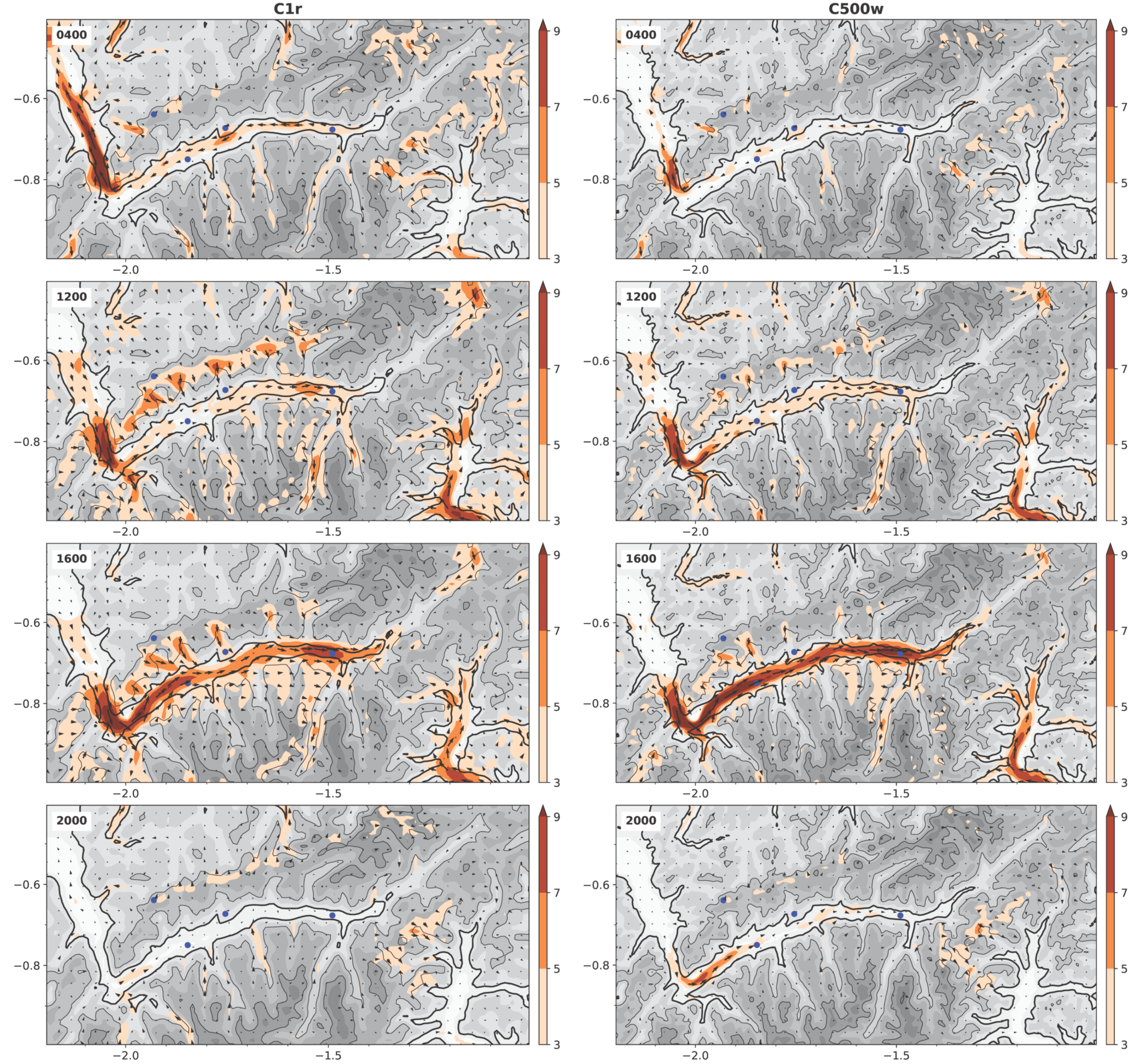
  • Of all four simulations, the C500w simulation was closest to the observed evolution of the winds and temperature in the valley atmosphere. Higher resolution alone did not result in improved results for the Sion region (in fact, the skill of C500r was lower than that for C1w). This finding highlights the importance of an accurate simulation of the temperature structure of the valley atmosphere as a prerequisite for the accurate representation of the valley wind system in the Sion region. The finer grid spacing helped to reproduce a stronger and more homogeneous along-valley wind and a more realistic cross-valley flow;
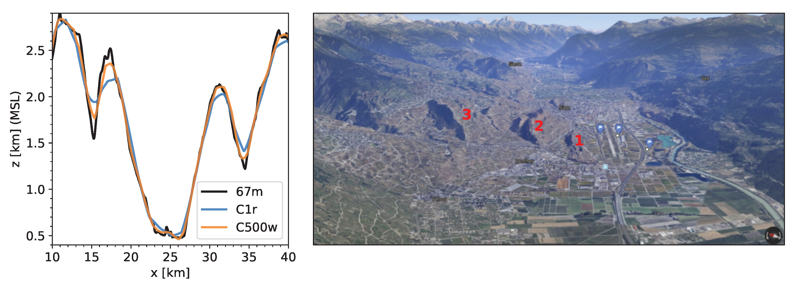
  • While C500w captures well the strength of the up-valley wind jet maximum (at 200 m AGL), the amplitude and timing of the near-surface (10 m) wind still deviate significantly from the observed evolution. This is attributed to the very local characteristics of the valley in the Sion region. Three small-scale hills to the northwest of Sion airport result in a constriction of the valley cross section and lead to an acceleration of the observed low-level flow (below 200–300 m AGL). A much higher model resolution with a horizontal grid spacing on the order of 100 m would be required for their adequate representation.
Our findings exhibit the complexity of the valley wind system in the region of Sion resulting from the superposition and interaction of a regular diurnal along-valley wind with a rather variable upper-level cross-valley wind, which is associated with a cross-regional flow from the Bernese Oberland to the drier inner-Alpine Wallis region. This cross-regional flow is highly variable in time, both on the sub-daily timescale as well as from day to day. Our results demonstrate the potential of high-resolution atmospheric models to represent these complex flow patterns and highlight the importance of an accurate representation of the temperature structure of the valley atmosphere and the characteristics and the state of the land surface, in particular for soil moisture, for the simulation of the boundary layer over complex terrain. Our study underlines the need for more comprehensive and detailed observations of the structure of the mountain atmosphere, the state of the land surface, and the exchange fluxes at the land–atmosphere interface, such as envisaged in [24], in order to guide the development of improved models and hence better forecasts of mountain weather.

Author Contributions

Conceptualization, J.S.; methodology, J.S.; software, J.S.; validation, J.S. and J.Q.-D.; formal Analysis, J.S.; Investigation, J.S. and J.Q.-D.; Resources, J.S.; Data Curation, J.S.; Writing—Original Draft Preparation, J.S. and J.Q.-D.; Writing—Review & Editing, J.S. and J.Q.-D.; Visualization, J.S.; Supervision, J.S.; Project Administration, J.S.; Funding Acquisition, J.S. All authors have read and agreed to the published version of the manuscript.

Funding

This research was funded by the Hans Ertel Centre for Weather Research of DWD (3rd phase, The Atmospheric Boundary Layer in Numerical Weather Prediction) Grant No. 4818DWDP4 and by the Deutsche Forschungsgemeinschaft (DFG, German Research Foundation)—TRR 301—Project-ID 428312742.

Data Availability Statement

The COSMO codes and data of the initial and lateral boundary conditions are available upon request with permission from the Deutscher Wetterdienst (DWD). The observational data are available on request from the original data providers.

Acknowledgments

This work used resources of the Deutsches Klimarechenzentrum (DKRZ) granted by its Scientific Steering Committee (WLA) under project ID bb1096. We would like to thank Ludovic Ranaud and Antoine Vessaz from MeteoSwiss for organizing the measurement campaign and for taking care of the instruments during the deployment. We further thank Dominique Ruffieux, former collaborator of MeteoSwiss, for thorough quality checking of the windprofiler data. Analyses and figures were produced using the open source software Python and Matplotlib [25].

Conflicts of Interest

The authors declare no conflict of interest.

Abbreviations

The following abbreviations are used in this manuscript:
AGLAbove ground level
SwissMetNetMeteoSwiss automatic monitoring network
C1rCOSMO 1.1 km grid spacing and COSMO-1 analysis soil moisture
C1wCOSMO 1.1 km grid spacing and increased initial soil moisture (+30%)
C500rCOSMO 0.5 km grid spacing and COSMO-1 analysis soil moisture
C500wCOSMO 0.5 km grid spacing and increased initial soil moisture (+30%)
CEVTown of Cevio
COSMOConsortium for Small-scale Modelling
MAEMean absolute error
MSLMean sea level
SIOTown of Sion
VISTown of Visp

Appendix A. Evaluation of Diurnal Pressure Amplitude

It has been shown that an accurate simulation of the stratification of the valley atmosphere is important for the accurate simulation of the valley wind system. Here, we would like to further evaluate the accuracy of the two key simulations C1r and C500w. Routine observations of the temperature structure are, however, sparse in space and time. Switzerland has only one routine radiosonde observation site located in Payerne. Soundings are launched twice a day at 00:00 and 12:00 UTC. To fill the gap in space and time and to obtain a first impression of the bulk representation of the diurnal cycle of temperature in the atmospheric boundary layer (ABL), we consider surface pressure measurements. These are available at over 100 stations in Switzerland with high temporal resolution. Assuming slowly varying large-scale conditions that is a slow variation of the pressure above the ABL, the diurnal heating and cooling of the ABL are imprinted on the evolution of the surface pressure [26,27]. In addition, the magnitude of the diurnal pressure amplitude is a measure of the magnitude of the diurnal bulk temperature change within the ABL. The ratio of the simulated to the observed diurnal pressure amplitude is shown in Figure A1. It can be seen that the pressure amplitude is strongly overestimated in C1r, in particular over the Alpine regions. The pressure amplitude is much better represented in C500w, both in the Alpine valleys and over the Swiss Plateau. Over the Swiss Pleateau, only a slight positive bias remains on average. Significant differences remain for a subset of the stations in the Alpine region. This requires further investigation which is beyond the scope of this study.
Figure A1. Evaluation of simulated diurnal pressure amplitude: Deviation (in %) of the ratio of the simulated to the observed mean diurnal pressure amplitude from the identify (average over the 18 valley wind days in September 2016) for the Swiss stations.
Meteorology 02 00007 g0a1

Appendix B. Further Sensitivity Experiments

For the sake of completeness, we include a partial list of the additional sensitivity experiments carried out during the investigation of the wind biases in the Sion region. These included simulations
  • with a reduced initial soil moisture (−30%);
  • with the shallow convection scheme turned on (itype_conv=3);
  • with different parameterization choices for the soil–vegetation–atmosphere interface;
    -
    including a skin layer (itype_canopy=2) and changing the skin layer conductivity (cskinc);
    -
    different parameterization options for soil heat conduction (itype_headcond);
    -
    different parameterization options for bare soil evaporation (itype_evsl);
  • with different parameterization choices for turbulence,
    -
    changing the minimum diffusion coefficient (tkmmin, tkhmin);
    -
    parameterization of subgrid-scale katabatic winds (pat_len);
  • and a larger model domain size,
where the names within the parentheses denote the COSMO namelist variables involved in the corresponding changes. While some of these experiments did have a significant impact on certain aspects of the flow, such as, for example, the near-surface temperature evolution, they did not have any significant impact on the wind biases in the region of Sion, with the exception of the experiment with a reduced initial soil moisture. The latter resulted in poorer results than for C1r. As these experiments did not have a positive impact on the winds at Sion in comparison to C1r and as most of them were carried out with an earlier model setup, not 100% consistent with the setup used for the four main simulations, we do not provide any quantitative assessment.

References

  1. Whiteman, C.D. Mountain Meteorology: Fundamentals and Applications; Oxford University Press: Oxford, UK, 2000. [Google Scholar]
  2. Zardi, D.; Whiteman, C. Diurnal mountain wind systems. In Mountain Weather Research and Forecasting: Recent Progress and Current Challenges; Chow, F.K., De Wekker, S.F.J., Snyder, B.J., Eds.; Springer: Berlin/Heidelberg, Germany, 2013; pp. 35–119. [Google Scholar]
  3. Schmidli, J. Daytime heat transfer processes over mountainous terrain. J. Atmos. Sci. 2013, 70, 4041–4066. [Google Scholar] [CrossRef]
  4. Rotach, M.W.; Wohlfahrt, G.; Hansel, A.; Reif, M.; Wagner, J.; Gohm, A. The world is not flat: Implications for the global carbon balance. Bull. Am. Meteorol. Soc. 2014, 95, 1021–1028. [Google Scholar] [CrossRef]
  5. Leukauf, D.; Gohm, A.; Rotach, M.W.; Wagner, J.S. The impact of the temperature inversion breakup on the exchange of heat and mass in an idealized valley: Sensitivity to the radiative forcing. J. Appl. Meteorol. Climatol. 2015, 54, 2199–2216. [Google Scholar] [CrossRef]
  6. Serafin, S.; Adler, B.; Cuxart, J.; De Wekker, S.F.; Gohm, A.; Grisogono, B.; Kalthoff, N.; Kirshbaum, D.J.; Rotach, M.W.; Schmidli, J.; et al. Exchange processes in the atmospheric boundary layer over mountainous terrain. Atmosphere 2018, 9, 102. [Google Scholar] [CrossRef]
  7. Lehner, M.; Rotach, M.W.; Obleitner, F. A method to identify synoptically undisturbed, clear-sky conditions for valley-wind analysis. Bound. Layer Meteorol. 2019, 173, 435–450. [Google Scholar] [CrossRef]
  8. Schmidli, J.; Böing, S.; Fuhrer, O. Accuracy of simulated diurnal valley winds in the Swiss Alps: Influence of grid resolution, topography filtering, and land surface datasets. Atmosphere 2018, 9, 196. [Google Scholar] [CrossRef]
  9. Chow, F.K.; Weigel, A.P.; Street, R.L.; Rotach, M.W.; Xue, M. High-Resolution Large-Eddy Simulations of Flow in a Steep Alpine Valley. Part I: Methodology, Verification, and Sensitivity Experiments. J. Appl. Meteorol. Climatol. 2006, 45, 63–86. [Google Scholar] [CrossRef]
  10. Liu, Y.; Liu, Y.; Muñoz-Esparza, D.; Hu, F.; Yan, C.; Miao, S. Simulation of flow fields in complex terrain with WRF-LES: Sensitivity assessment of different PBL treatments. J. Appl. Meteorol. Climatol. 2020, 59, 1481–1501. [Google Scholar] [CrossRef]
  11. Schmidli, J.; Poulos, G.S.; Daniels, M.H.; Chow, F.K. External influences on nocturnal thermally driven flows in a deep valley. J. Appl. Meteorol. Climatol. 2009, 48, 3–23. [Google Scholar] [CrossRef]
  12. Schmid, F.; Schmidli, J.; Hervo, M.; Haefele, A. Diurnal valley winds in a deep alpine valley: Observations. Atmosphere 2020, 11, 54. [Google Scholar] [CrossRef] [Green Version]
  13. Steppeler, J.; Doms, G.; Schättler, U.; Bitzer, H.; Gassmann, A.; Damrath, U.; Gregoric, G. Meso-gamma scale forecasts using the nonhydrostatic model LM. Meteorol. Atmos. Phys. 2003, 82, 75–96. [Google Scholar] [CrossRef]
  14. Klemp, J.B.; Wilhelmson, R.B. The simulation of three-dimensional convective storm dynamics. J. Atmos. Sci. 1978, 35, 1070–1096. [Google Scholar] [CrossRef]
  15. Wicker, L.J.; Skamarock, W.C. Time-splitting methods for elastic models using forward time schemes. Mon. Weather. Rev. 2002, 130, 2088–2097. [Google Scholar] [CrossRef]
  16. Reinhardt, T.; Seifert, A. A three-category ice scheme for LMK. In COSMO Newsletter, No. 6, Consortium for Small-Scale Modeling; Deutsche Wetterdienst: Offenbach, Germany, 2006; pp. 115–120. [Google Scholar]
  17. Ritter, B.; Geleyn, J.F. A comprehensive radiation scheme for numerical weather prediction models with potential applications in climate simulations. Mon. Weather. Rev. 1992, 120, 303–325. [Google Scholar] [CrossRef]
  18. Mellor, G.L.; Yamada, T. Development of a turbulence closure model for geophysical fluid problems. Rev. Geophys. 1982, 20, 851–875. [Google Scholar] [CrossRef]
  19. Raschendorfer, M. The new turbulence parameterization of LM. In COSMO Newsletter, No. 1, Consortium for Small-Scale Modeling; Deutsche Wetterdienst: Offenbach, Germany, 2001; pp. 89–97. [Google Scholar]
  20. Baldauf, M.; Seifert, A.; Förstner, J.; Majewski, D.; Raschendorfer, M.; Reinhardt, T. Operational Convective-Scale Numerical Weather Prediction with the COSMO Model: Description and Sensitivities. Mon. Weather. Rev. 2011, 139, 3887–3905. [Google Scholar] [CrossRef]
  21. Schulz, J.P.; Vogel, G.; Becker, C.; Kothe, S.; Ahrens, B. Evaluation of the ground heat flux simulated by a multi-layer land surface scheme using high-quality observations at grass land and bare soil. In Proceedings of the EGU General Assembly Conference Abstracts, Vienna, Austria, 12–17 April 2015; p. 6549. [Google Scholar]
  22. Hohenegger, C.; Brockhaus, P.; Bretherton, C.S.; Schär, C. The soil moisture-precipitation feedback in simulations with explicit and parameterized convection. J. Clim. 2009, 22, 5003–5020. [Google Scholar] [CrossRef]
  23. Kaufmann, P. Association of surface stations to NWP model grid points. In COSMO Newsletter, No. 9.2, Consortium for Small-Scale Modeling; Deutsche Wetterdienst: Offenbach, Germany, 2008. [Google Scholar]
  24. Rotach, M.W. A collaborative effort to better understand, measure, and model atmospheric exchange processes over mountains. Bull. Am. Meteorol. Soc. 2022, 103, E1282–E1295. [Google Scholar] [CrossRef]
  25. Hunter, J.D. Matplotlib: A 2D graphics environment. Comput. Sci. Eng. 2007, 9, 90–95. [Google Scholar] [CrossRef]
  26. Y, L.; Smith, R.B.; Grubisic, V. Using surface pressure variations to categorize diurnal valley circulations: Experiments in Ownes Valley. Mon. Weather. Rev. 2009, 137, 1753–1769. [Google Scholar]
  27. Schmidli, J.; Rotunno, R. Mechanisms of along-valley winds and heat exchange over mountainous terrain. J. Atmos. Sci. 2010, 67, 3033–3047. [Google Scholar] [CrossRef] [Green Version]
Figure 1. (a) Model integration domain and terrain height (m; shaded); (b) location of the diurnal wind stations available in September 2016 (black diamonds), of two extra stations in the Wallis (DIA, MVE), and of the site of the radiosonde ascent (PAY). Sion and three stations in the Wallis are highlighted in blue. The black line denotes the footprint of the vertical cross section discussed in Section 3.5.
Meteorology 02 00007 g001
Figure 2. Overview of weather conditions during September 2016 from observations (black), and the reference simulation C1r (blue); based on an average over the valley-wind stations (ac) and the twice-daily Payerne radiosonde data (d,e). Time series of (a) mean precipitation, (b) global radiation, (c) 2 m temperature, (d) potential temperature at 2000 m AGL (thin lines) and 4000 m AGL (thick lines), and (e) wind speed (lines) and wind direction (symbols) at 4000 m AGL. The orange lines in (a) denote the valley wind days.
Meteorology 02 00007 g002
Figure 3. Mean diurnal cycle of key surface variables averaged over the valley wind days in September 2016 from observations and simulations, averaged over the valley wind stations (top row) and for Sion (bottom row). The variables shown include the incoming solar radiation (swd), the 2 m temperature (Tc), the 2 m dew point temperature (Td), and the 2 m relative humidity (rh).
Meteorology 02 00007 g003
Figure 4. Mean diurnal cycle of wind speed (lines) and wind direction (symbols) for the valley wind days in September 2016 from observations and simulations for three locations: Visp (VIS), a station in a typical large valley, Cevio (CEV), a station in a typical small valley, and Sion (SIO). As indicated in Section 2.3, the mean wind speed and direction are calculated by vector averaging the hourly wind vectors.
Meteorology 02 00007 g004
Figure 5. Root mean square error (RMSE) of the mean up-valley wind (10:00–14:00) for the main simulations.
Meteorology 02 00007 g005
Figure 6. Mean diurnal cycle of the valley wind (vector-averaged) for the valley-wind days in September 2016 from observations and simulations for the location of Sion. Observations are based on a combination of the low-mode wind profiler and the weather station data. The filled contours indicate the along-valley wind speed (m/s) with positive values for up-valley wind, and the barbs denote the wind direction with respect to the valley’s axis. The wind speed is masked if more than 50% of the values are missing and wind barbs are plotted if the wind speed is greater than 2.5 knots.
Meteorology 02 00007 g006
Figure 7. Vector-averaged profiles of the mean (a) down-valley wind at 08:00 and (b) up-valley wind at 16:00, for the valley wind days for observations (low-mode wind profiler) and simulations (C1r and C500w) for the location of Sion; (c) bias and mean absolute error (MAE) of hourly wind speeds (solid) and hourly wind velocities (dashed) during the 18 valley wind days with respect to the high-mode wind profiler. Grey points represent the data availability, which at the surface is 100%. Note that the high-mode data are used for the statistics (including data availability) due to poor data availability of the low-mode data at higher elevations, but the low-mode data is used for the profiles in order to resolve the low-level jet.
Meteorology 02 00007 g007
Figure 8. Local conditions at Sion. Left panel: Terrain height along the valley cross-section shown in Figure 1 at three different resolutions: original ASTER data (67 m), filtered for 1 km simulations (C1), and for 500 m simulations (C500); Right panel: Three-dimensional view of the Sion area (Google Maps). The numbers indicate the location of the three small hills discussed in the text.
Meteorology 02 00007 g008
Figure 9. Mean diurnal cycle of the valley winds in Wallis for the valley wind days in September 2016. Wind speed (shading) and direction (vectors) at ca. 200 m AGL (10th model level). Time is indicated in the top left corner. Location of four surface stations (blue discs; see Figure 1). Gray shading indicates the terrain height (500 m contour interval) and the bold black line indicates the 1000 m contour.
Meteorology 02 00007 g009
Figure 10. Snapshot of the flow pattern on 23 September 2016 at 16:00 for three different simulations. (Left column) Wind speed (shading) and direction (vectors) at ca. 200 m AGL (10th model level); (Right column) Along- valley wind component normal to the cross-section (shading), potential temperature (black contours), and cross-valley wind (vectors; wind component parallel to the cross-section) in a vertical cross section through Sion (see Figure 1).
Meteorology 02 00007 g010
Figure 11. As in Figure 10, but for 10 September 2016 at 16:00.
Meteorology 02 00007 g011
Figure 12. Time-height plot of the along-valley wind speed (shading) and wind direction (barbs) relative to the valley’s axis for the low-mode wind profiler (OBS) and three model runs for 10 September 2016.
Meteorology 02 00007 g012
Figure 13. Structure of the valley atmosphere at Sion for 10 September 2016 at 16:00: (a) wind speed and wind direction; (b) potential temperature (solid lines) and specific humidity (dashed lines); (c) evaluation of the mean temperature and moisture structure at Payerne at 12 UTC, average over the 18 valley wind days. The grey dashed lines in the panel showing wind direction indicate the up- and down-valley direction, respectively.
Meteorology 02 00007 g013
Figure 14. Comparison of observed and simulated bulk stratification of the valley atmosphere, based on observed and simulated temperature at the stations Sion (482 m MSL), Montana (1427 m MSL), and Les Diablerets (2964 m MSL). Stratification over the entire valley depth is given by the potential temperature difference between Les Diablerets and Sion (solid curves); stratification of the lower part of the valley depth is given by the difference between Montana and Sion. (a) Time series of the stratification for the period 9–11 September 2016; (b) mean diurnal cycle of the stratification for the valley wind days.
Meteorology 02 00007 g014
Table 1. Summary of the main numerical experiments. Slope refers to the maximum slope in the integration domain.
Experiment Δ x Δ t Initial Soil MoistureSlope
(m)(s)( )
C1r110010COSMO-1 analysis43.6
C1w110010+30%43.6
C500r5505COSMO-1 analysis45.9
C500w5505+30%45.9
Disclaimer/Publisher’s Note: The statements, opinions and data contained in all publications are solely those of the individual author(s) and contributor(s) and not of MDPI and/or the editor(s). MDPI and/or the editor(s) disclaim responsibility for any injury to people or property resulting from any ideas, methods, instructions or products referred to in the content.

