

Evaluation of Future Simulations of the CMIP5 GCMs Concerning Boreal Wintertime Atmospheric Teleconnection Patterns


Department of Meteorology, Institute of Geography and Earth Sciences, ELTE Eötvös Loránd University, Pázmány Péter Sétány 1/A, 1117 Budapest, Hungary
Meteorology 2022, 1(4), 450-467; https://doi.org/10.3390/meteorology1040028
Submission received: 5 September 2022
/
Revised: 16 October 2022
/
Accepted: 1 November 2022
/
Published: 7 November 2022
(This article belongs to the Special Issue Early Career Scientists' (ECS) Contributions to Meteorology (2022))
Abstract
:In this study, a pattern detection method is applied on the RCP4.5 and RCP8.5 simulation outputs of seven GCMs—disseminated by the Coupled Model Intercomparison Project Phase 5 (CMIP5)—to determine whether atmospheric teleconnection patterns detected in the ERA-20C reanalysis from the European Centre for Medium-Range Weather Forecasts (ECMWF) will be observable in the future projections of the CMIP5 GCMs. The pattern detection technique—which combines the negative extrema method and receiver operating characteristic (ROC) curve analysis—is used on the geopotential height field at the 500 hPa pressure level in wintertime, in the Northern Hemisphere. It was found that teleconnections obtained from the ERA-20C reanalysis dataset for the period of 1976–2005 remain observable in the majority of the GCM outputs under the RCP4.5 and RCP8.5 scenarios for the periods of 2006–2035, 2021–2050, and 2071–2100. The results imply that atmospheric internal variability is the major factor that controls the teleconnections rather than the impact of radiative forcing.
1. Introduction
Atmospheric teleconnections—henceforth teleconnections—are considered as simultaneous correlations in the field of some meteorological variable, e.g., in the geopotential height field [1,2]. The action centers—hereinafter referred to as ACs—are the regions of teleconnections associated with the strongest correlations, e.g., [1,3].
Since atmospheric circulation phenomena on different scales are not independent from each other, large-scale phenomena can affect the climate of smaller regions [4]. Local climate anomalies are often related to large-scale anomalies via teleconnections [5]. For example, variability of the midlatitude jet stream over the Euro-Atlantic region are related to the occurrence of atmospheric blockings—henceforth blockings—[6], which can be described by the North Atlantic Oscillation (NAO) and the East Atlantic (EA) pattern [7,8]. The Pacific-North American (PNA) pattern is associated with Pacific and Atlantic blockings [9].
Weather and climate extremes—e.g., the frequency and intensity of wildfires, precipitation extremes, floods, and dry spells—are influenced by blockings [10], thus by teleconnections. Concerning teleconnections which can be detected on the geopotential height field at the 500 hPa pressure level (abbreviated as zg500) in the Northern Hemisphere (NH), the NAO and the Western Mediterranean Oscillation (WeMO) were linked to the occurrence of wildfires over the western part of the Mediterranean region [11]. Ref. [12] examined the impact of teleconnections—among others the Eurasian (EU) pattern—on extreme rainfall events in China. In boreal wintertime, the PNA pattern was linked to precipitation extremes over the West Coast of the United States [13], while the NAO and the Mediterranean Oscillation (MO) were associated with longer extreme dry spells in the Mediterranean region [14].
Since the frequency and intensity of weather and climate extremes, such as hot extremes and heavy precipitation, had increased under climate change [15,16], it is crucial to predict how the teleconnections will alter through the 21st century. Teleconnections represent the internal variability of the climate system [17], however, external forces—originated from the ocean, the troposphere, and the stratosphere—may also affect the teleconnections [18,19].
General circulation models (GCMs)—which represent the dynamics of the ocean and the atmosphere [16]—have been used extensively to study teleconnections and their future changes under different scenarios. (1) Based on model simulation results, [20,21] pointed out that anthropogenic greenhouse gas (GHG) forcing may cause positive trend in the NAO observations and north-eastward shift in its ACs, while [22] found that a negative trend is associated with the westward shift of the ACs. More recent studies [23,24] showed that positive trend is linked to internal variability rather than anthropogenic forcing. (2) However, anthropogenic forcing modulates the interannual variability of the midlatitude jet stream in the North Atlantic region in connection with the EA pattern and the NAO [8]. (3) Based on GCM simulations, [25] described the poleward expansion of the Hadley cell, while [26] named the GHGs and stratospheric ozone depletion as the main reasons of that. According to [27], the widening of the Hadley cell is linked to teleconnections like the NAO. (4) Blockings are linked to the NAO and the PNA in the North Atlantic and Pacific basins [28], consequently eastward shift of the blockings in the NH in wintertime [29] may affect the teleconnections significantly. (5) Based on the examination of high-resolution GCM simulations by [30], the Atlantic Meridional Overturning Circulation (AMOC)—that is linked to the NAO—likely continues to weaken under global warming, which implies the weakening of the NAO. The MO relates the NAO [31], therefore, changes in the NAO may lead to changes in the atmospheric circulation and the hydrological cycle of the Mediterranean region [32,33].
The main goal of this paper is to demonstrate that the pattern detection algorithm—published in [34]—can be applied on the future projections of the GCMs to identify teleconnection patterns. Furthermore, maps of the teleconnection patterns are examined whether teleconnections identified in the last decades of the 20th century, in [34,35], remain observable at the end of the 21st century. The summary of the method can be found in Section 2, while the results of the comparison are presented in Section 3. It is followed by the Discussion and the Conclusion in Section 4 and Section 5, respectively.
2. Data and Methods
In this paper the future projections of seven GCMs disseminated by the World Climate Research Programme (WCRP) Coupled Model Intercomparison Project Phase 5 (CMIP5) [17] were examined (listed in Table 1), which were created under the Representative Concentration Pathways (RCP) [36] scenarios RCP4.5 and RCP8.5. Three 30-year-long time periods were chosen for the analysis: 2006–2035, 2051–2080, and 2071–2100.
For the analysis, daily gridded zg500 time series were examined for winter months (December, January, and February) in the NH. The 31st days of the months and leap days were removed for the consistency of GCMs, therefore, each time series included 2640 data. The time series were deseasonalized by removing their long-term average and dividing them by their long-term standard deviation. The linear trend was also removed from each time series. Bilinear interpolation was used to interpolate the gridded data to a common grid with the resolution of 2.5° which contains 5328 grid cells.
By applying the pattern detection algorithm published in [34], maps of cluster patterns—abbreviated as CP maps—were constructed, which capture the signs of teleconnections. The GCM CP maps were compared against the CP map obtained from the European Centre for Medium-Range Weather Forecasts (ECMWF) twentieth century reanalysis (ERA-20C) dataset [45] for the period of 1976–2005, called as reference CP map.
The CP maps were constructed based on the negative extrema method [1,46]. In the first step, fields of the strongest negative correlations—abbreviated as SNC fields—were created as follows: In the case of each GCM simulation, the Pearson correlation coefficients—henceforth correlations—were computed between any possible pair of the time series. The SNC was selected in every grid cell. Due to the long time series, relatively low correlations (<−0.3) can be considered as significant at a significance level of 0.001, according to the results of the permutation test. Grid cells were identified as potential ACs if those were associated with the same correlation in the SNC field (see Figure 1a).
In the second step, the 2.5th, 5th, etc., 97.5th percentiles of the correlations were determined in case of each SNC field. Then, the SNC fields were masked as follows: if a grid cell was associated with a correlation below (above) the given percentile, then it was coded with 1 (0). Neighboring grid cells with the associated value of 1 formed a cluster. The clusters were merged which were in connection with each other by at least one pair of potential ACs. Those clusters are considered as the imprints of the teleconnections. The pair of potential ACs associated with the most intense negative correlation in each cluster was identified as the AC of the cluster/teleconnection. Finally, a total of 7·39 GCM CP maps were created for each examined time period, under the RCP4.5 and the RCP8.5 scenarios, respectively. More details about the pattern detection algorithm and an example are available in [34], while details about the applied permutation test can be found in [35].
The GCM CP maps were compared to the reference CP map which was selected in accordance with [34] (see Figure 1b). The comparison was done by constructing the receiver operating characteristic (ROC) curve for each GCM as follows. The false positive rate (FPR) on the x-axis was plotted against the true positive rate (TPR) on the y-axis which were calculated by the following formulas (see e.g., [47]):
where
- True positive (TP) means that the grid cell in the GCM CP map and in the reference CP map belong to the same cluster,
- True negative (TN) means that the grid cell in the GCM CP map and in the reference CP map does not belong to any a cluster,
- False positive (FP) means that the grid cell belongs to a cluster in the GCM CP map, which is not true for the reference CP map, and
- False negative (FN) means that the grid cell does not belong to any cluster in the GCM CP map, while it belongs to a cluster in the reference CP map.
As the measure of similarity between the GCM CP maps and the reference CP map, the area under the ROC curve—i.e., the AUC value—was calculated.
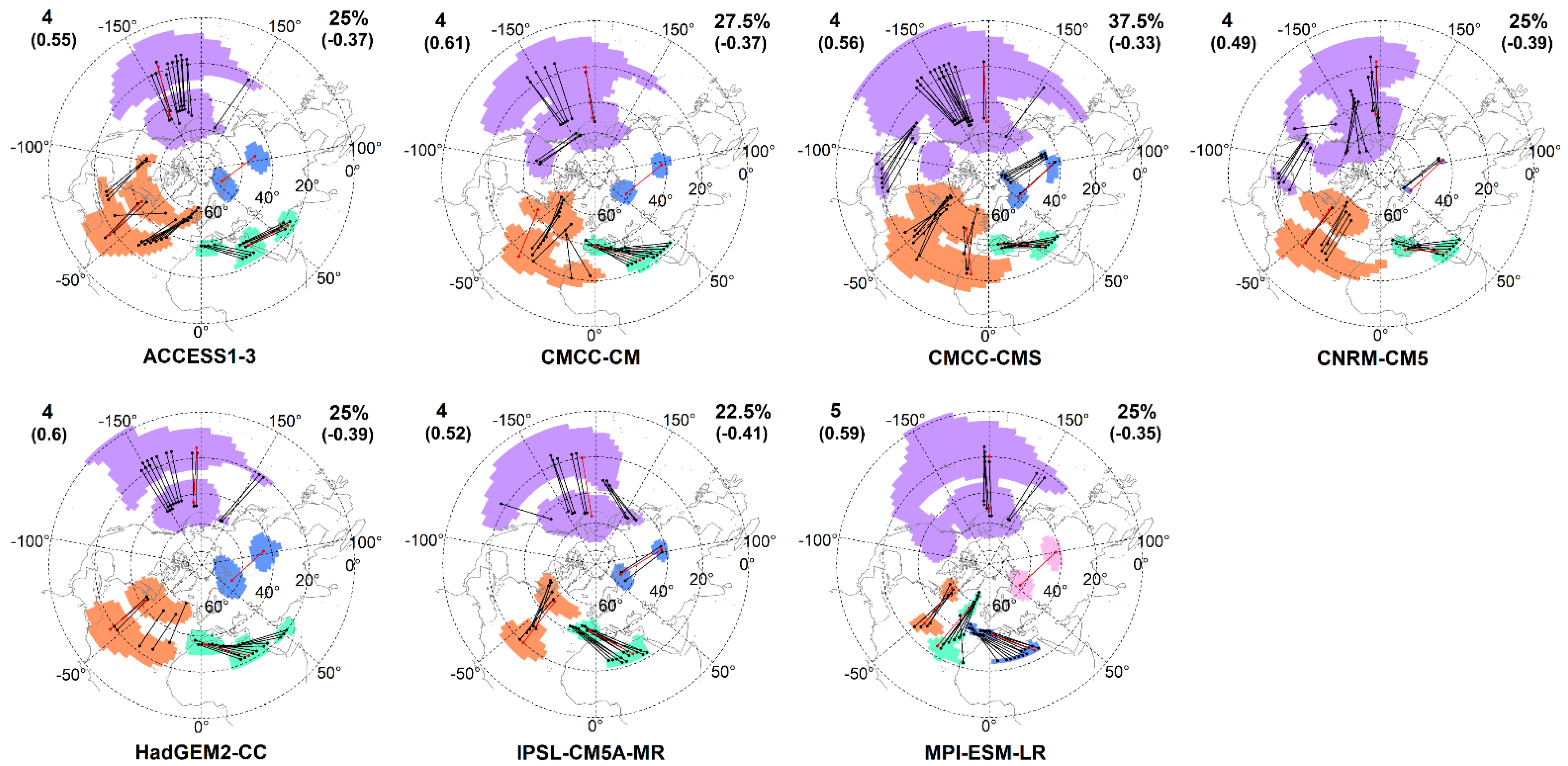
The reference CP map contains clusters with ACs geographically closest to the AC of the teleconnections described by [1,48].
Teleconnections were analyzed in the GCM CP maps which are the most similar to the reference CP map—for each GCM, for each time period, and for each RCP scenario, by computing the Matthews correlation coefficient (MCC) according to the following formula [49]:
The MCC values vary between −1 and 1. The value 1 means perfect match between the GCM CP map and the reference CP map, therefore only TP or TN values differ from zero. The value -1 indicates complete mismatch, consequently only FP and FN values differ from zero. The most similar GCM CP map was selected from those maps, which contain clusters in similar positions as clusters in the reference CP map, and which was associated with the largest MCC value (MCCmax).
Preprocessing of the climate data was done by using Climate Data Operators (CDO) [50], while the SNC fields and CP maps were created by applying R programming language [51]. The R packages ncdf4 [52], maps [53], mapproj [54], RColorBrewer [55], and magick [56] were used. R scripts are accessible in the GitHub repository of the author: https://github.com/ekristof86/R_codes_related_to_atmospheric_teleconnections (last accessed on 15 October 2022). R functions matrix.poly and val2col were also used for data visualization, which are available in the websites (last accessed on 15 October 2022): http://menugget.blogspot.com/2012/04/create-polygons-from-matrix.html, and http://menugget.blogspot.com/2011/09/converting-values-to-color-levels.html.
3. Results
3.1. General Overview of the SNC Fields
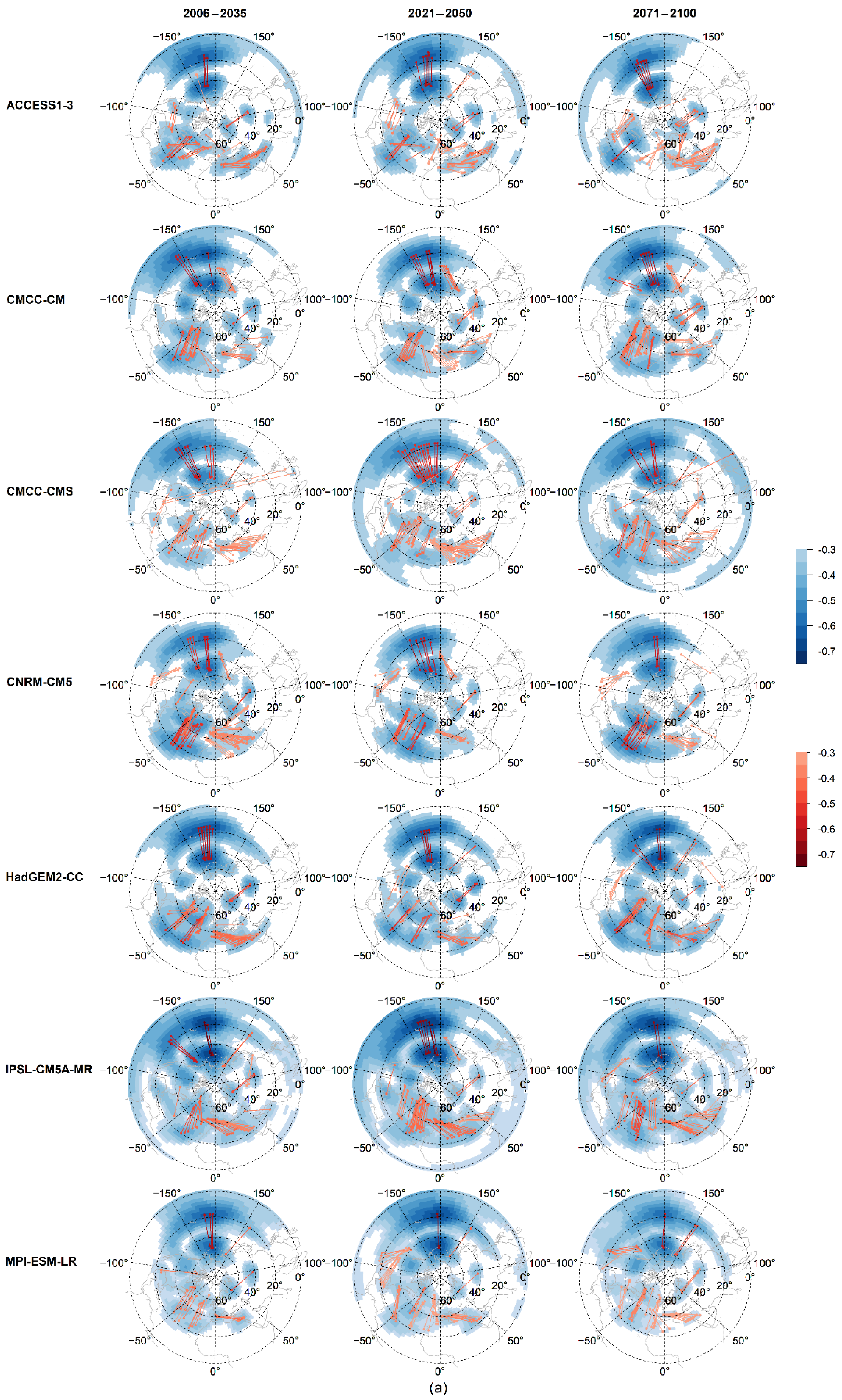
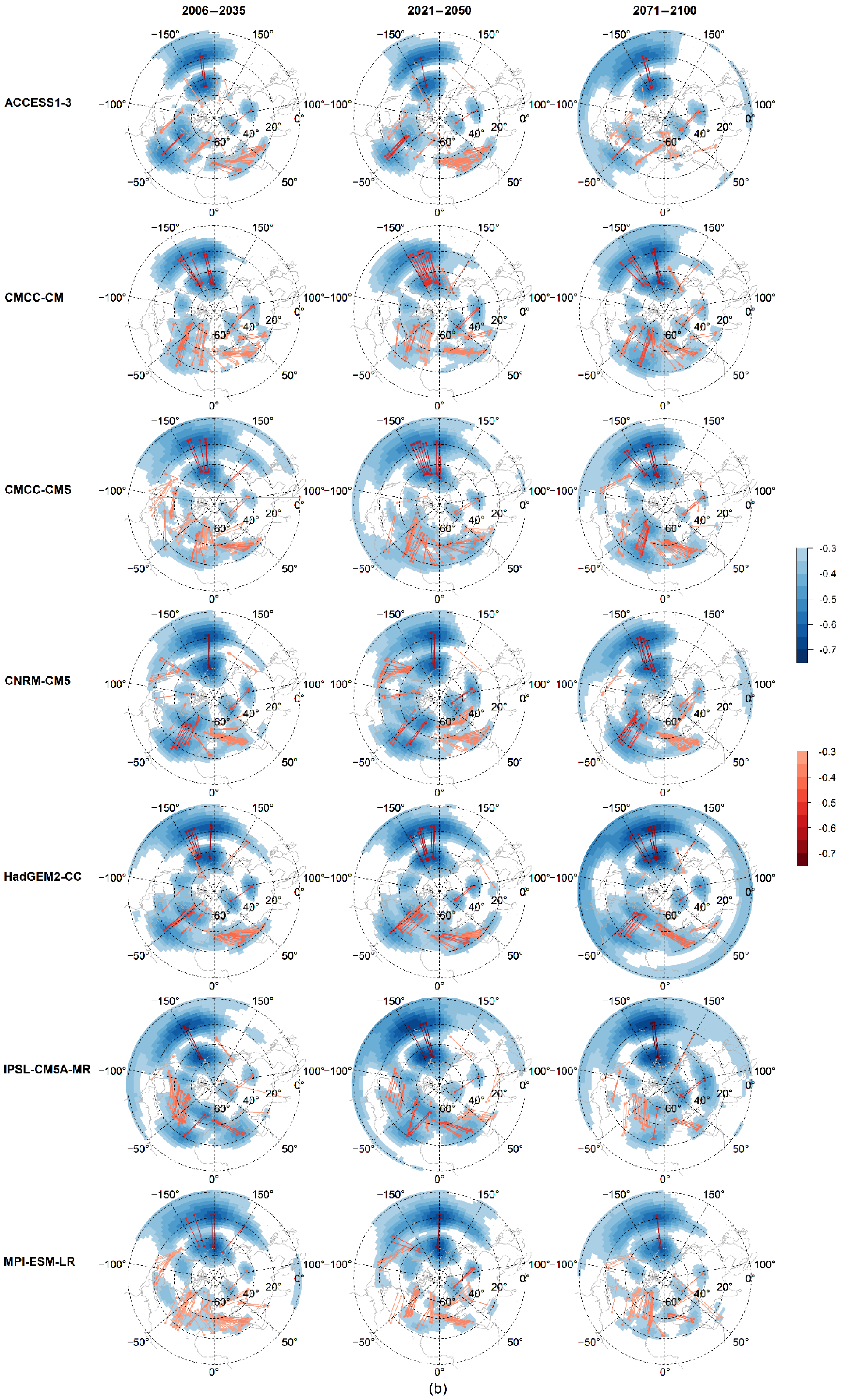
The SNC fields obtained from the GCM projections are shown in Figure A1. The local minima of the SNC fields obtained from the GCMs are in similar geographical areas as in the reference SNC field, obtained from the ERA-20C (see Figure 1a). Those locate over the North Pacific Ocean and North America (abbreviated as the North Pacific region), over the North Atlantic Ocean, in the region of the Mediterranean Sea and the Red Sea (abbreviated as the Mediterranean region), and in the region of the West Siberian Plain and the Gobi Desert (abbreviated as Asia). The North Pacific region is covered by the most intense negative correlations in the SNC fields of all GCMs, similarly to the SNC field of the ERA-20C. The minimal and mean values of the SNCs vary between −0.56–−0.7, and between −0.31–−0.37 for each GCM, respectively.
Regarding the distribution and intensity of the SNCs, there are no significant differences between the RCP simulations/time periods. It is confirmed by the RMSE values computed from the SNC fields, which are smaller than 0.07 for all GCMs, while the largest difference between two grid cells is around 0.15, except for the HadGEM2-CC. The latter can be explained by the significant correlations which cover the SNC field along the Equator obtained from the RCP8.5. simulation outputs.
3.2. Examination of the GCM CP Maps
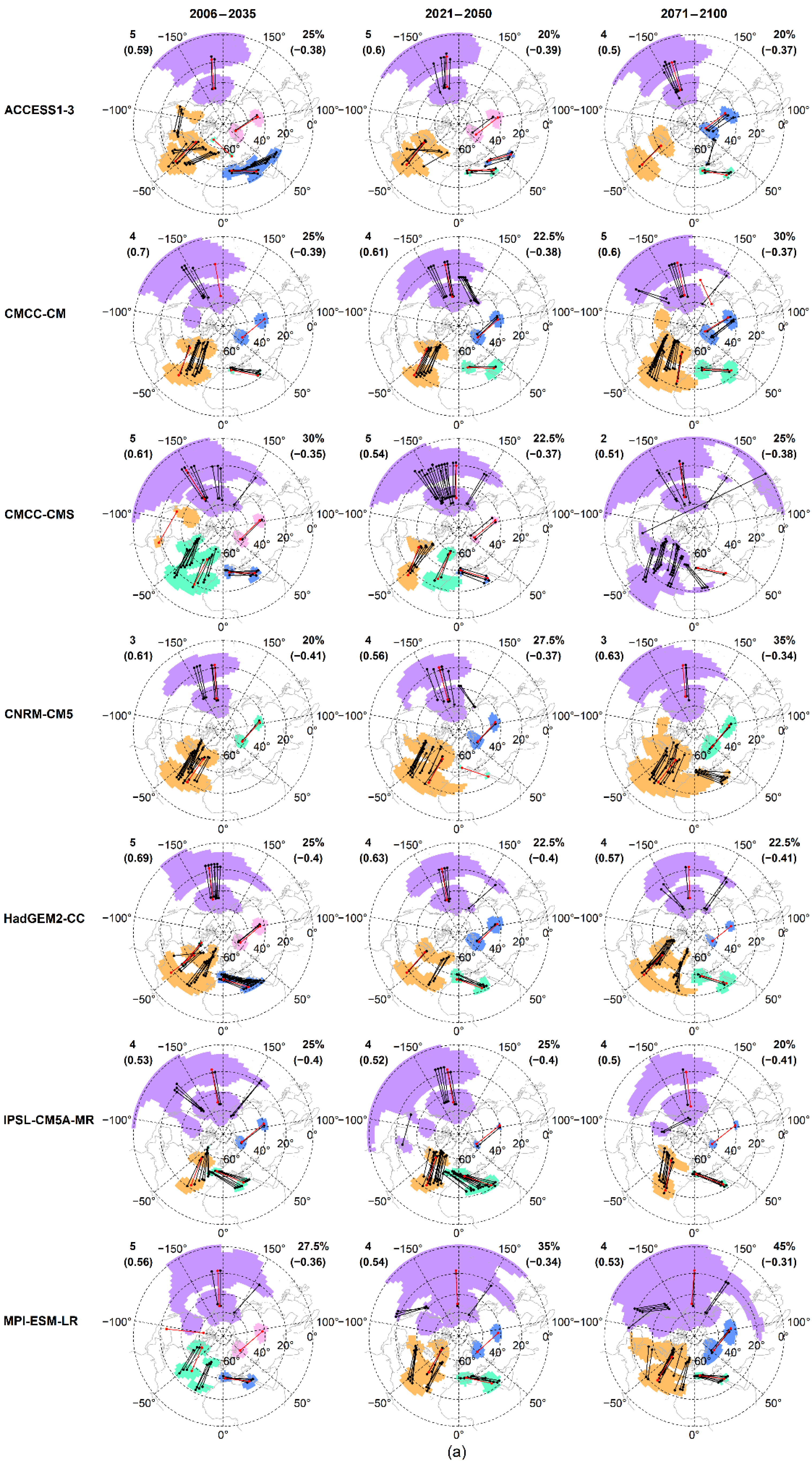
The GCM CP maps obtained from the RCP4.5 simulation outputs are presented in Figure 2a (The GCM CP maps based on the historical simulation outputs can be seen in Figure A2). Clusters/teleconnections over the North Pacific region and the North Atlantic Ocean, in the Mediterranean region and over Asia are observable in the vast majority of the GCM CP maps, in all examined time periods (i.e., in 19 cases of the presented 21 GCM CP maps). The exceptions are the CMCC-CMS for the period of 2071–2100 concerning the teleconnection over the North Atlantic Ocean and Asia and the CNRM-CM5 for the periods of 2006–2035 and 2071–2100 with respect to the teleconnection in the Mediterranean region. The largest agreement between the GCMs is in cases of the teleconnections over the North Pacific region and Asia. In cases of the CMCC-CM, the CNRM-CM5, the IPSL-CM5A-MR and the MPI-ESM-LR, the most intense regions of the teleconnections are in similar position through the 21st century. The GCMs show larger difference regarding the position of the ACs over the North Atlantic Ocean. The ACCESS1-3, the HadGEM2-CC, and the MPI-ESM-LR locate the most intense region of the teleconnection over the western part of the Atlantic Ocean, while the CMCC-CMS, the CNRM-CM5, and the IPSL-CM5A-MR locate them eastward. In the CP map of the CMCC-CMS for the period of 2071–2100 a unique “bridge” can be seen between the clusters of the two oceanic areas, which cannot be detected in any other CP maps. The teleconnection in the Mediterranean region is represented in the same area in the majority of the GCM simulation outputs, however in the CP map of the ACCESS1-3 two pairs of ACs can be detected, while in cases of the CMCC-CMS and the IPSL-CM5A-MR the most intense region of the teleconnection is closer to the teleconnection over the Atlantic Ocean.
Figure 2.
Maps of cluster patterns (CP maps) (a) obtained from the RCP4.5 simulations and (b) obtained from the RCP8.5 simulations, which are the most similar to the reference CP map obtained from the ERA-20C for the period of 1976–2005. Denotations are the same as in Figure 1b.
Figure 2.
Maps of cluster patterns (CP maps) (a) obtained from the RCP4.5 simulations and (b) obtained from the RCP8.5 simulations, which are the most similar to the reference CP map obtained from the ERA-20C for the period of 1976–2005. Denotations are the same as in Figure 1b.


GCM CP maps obtained from the RCP8.5 simulations are presented in Figure 2b. The teleconnections in the four regions mentioned above are also observable in the vast majority of the GCM CP maps. The most intense regions of the teleconnections—except for the teleconnection in the Mediterranean region—are in similar positions in the GCM CP maps obtained from the RCP4.5 and RCP8.5 simulation outputs. However, the clusters over the two oceanic regions tend to merge in some GCMs before the clusters in the Mediterranean region pop up, e.g., in case of the CNRM-CM5 and the HadGEM2-CC for the period of 2071–2100. The teleconnections over the North Atlantic Ocean and in the Mediterranean region merge at an early step of the clustering algorithm, e.g., in case of the IPSL-CM5A-MR for the periods of 2006–2035 and 2021–2050. There are GCM CP maps obtained from the RCP4.5 simulations in which the teleconnections over the North Atlantic Ocean and in the Mediterranean region are especially close to each other. Those teleconnections tend to merge in the GCM CP maps obtained from the RCP8.5 simulations. This can be seen in the CP maps of the HadGEM2-CC and the IPSL-CM5A-MR. The CP maps of the CMCC-CM significantly differ from each other concerning the teleconnection in the Mediterranean region, because a secondary intensity center appears in the CP map obtained from the RCP8.5 simulation outputs at an early step of the pattern detection algorithm, for the periods of 2006–2035 and 2021–2050.
3.3. Evaluation of the GCMs Based on the MCCmax and the AUC Values
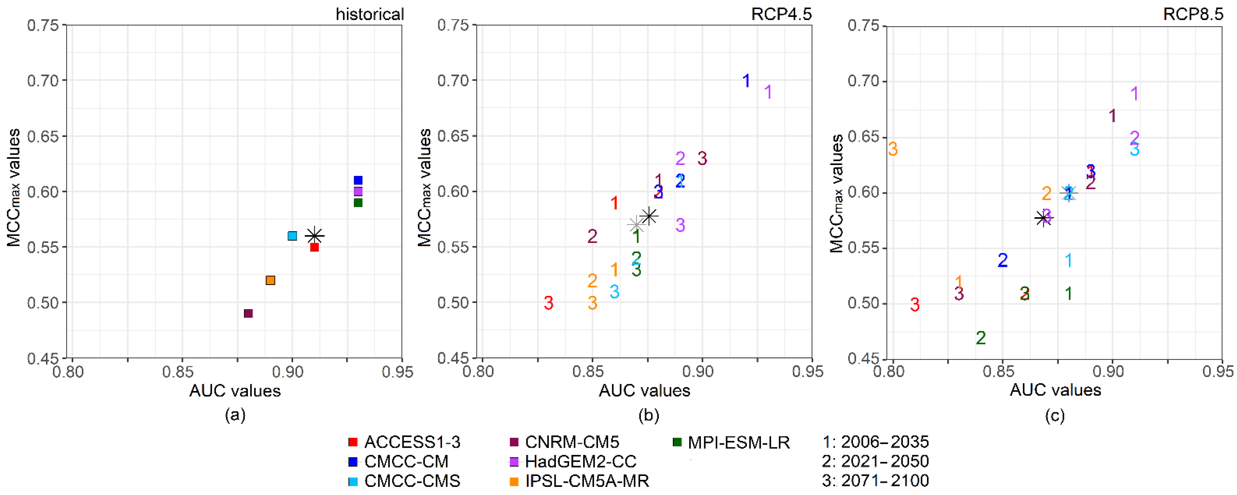
The simulations of the GCMs under the RCP4.5 and the RCP8.5 scenarios are evaluated based on their MCCmax and AUC values. The ROC curves are shown in Figure 3. The spreads of the ROC curves obtained from the RCP4.5 and the RCP8.5 simulations are similar; however, those increase over time for both in cases of the RCP4.5 and the RCP8.5 simulations.
The MCCmax and the AUC values are shown in Figure 4, while the corresponding data can be found in Table 2 and Table A1. The MCCmax values vary between 0.47 and 0.7 and the AUC values are between 0.8 and 0.93 in all cases. There are only slight differences between the MCCmax and the AUC values, respectively. If the MCCmax (AUC) values—based on the RCP4.5 and the RCP8.5 scenarios—are compared to each other in case of each GCM for all the three time periods, then the differences are below 0.14 (0.07). If the values are compared to each other based on the time periods, then a slight decrease—smaller than 0.12 (0.05) in cases of the MCCmax (AUC) values—can be detected from 2006–2035 to 2071–2100.
There is no GCM which overperforms all the other GCMs in all time periods. The CP maps of the HadGEM2-CC share large similarities with the reference CP map, except for the period of 2071–2100. The reason is the unique distribution of the SNCs mentioned in Chapter 3.1. According to Figure 4, the MCCmax and the AUC values have larger variability in case of the RCP8.5 scenario compared to the RCP4.5 scenario.
4. Discussion
The seven GCMs examined in this paper were chosen based on the validation results of their historical simulation outputs published in [34,35], where those GCMs performed the most reliable relative to reanalysis datasets. The period of 1976–2005 was chosen as the reference because it is the last 30-year-long period on which historical CMIP5 GCM data are available. Consequently, we assume that GCMs which perform well closer to the Millennia, remain accurate in the 21st century. Because of this assumption, the validation of the RCP simulation outputs will be an important task of the future [57,58].
In the GCM CP maps the clusters indicate the teleconnections identified by [1,48,59]. The clusters over the North Pacific region correspond to the PNA, while the clusters over the western and eastern parts of the North Atlantic Ocean indicate the West Atlantic (WA) and the EA patterns. The teleconnection over the Mediterranean region implies the MO, while the teleconnection over Asia can be corresponded to the EU pattern.
This study has several limitations linked to the pattern detection algorithm which are the followings. (1) Due to the coarse resolution of the percentile values—which were used as thresholds in the pattern detection algorithm—the GCM CP maps are not suitable in all cases to delimit two clusters—namely the WA and EA patterns—over the North Atlantic Ocean. With a finer resolution, the pattern detection algorithm described in [34] can be used to detect and delimit those teleconnections, in a reproducible way. (2) Because the pattern detection algorithm is based on the negative extrema method, this technique cannot be used to identify clusters/teleconnections with more than two ACs without subjective considerations [19]. Therefore, the pattern detection algorithm in this paper was restricted to identify teleconnections with two, negatively correlated ACs. This limitation is obvious in case of the PNA. Two pairs of ACs—one pair over the North Pacific Ocean, while the other pair over North America—form two separate clusters, which can be seen in the CP map of the CMCC-CMS under the RCP4.5 scenario, for the period of 2006–2035 (see Figure 2a), and the CP map of the IPSL-CM5A-MR under the RCP8.5 scenario for the period of 2021–2050 (see Figure 2b). To explore positive correlations, a useful tool can be the empirical orthogonal teleconnection (EOT) analysis [60] or its lagged version the multichannel EOT analysis [61]. (3) Furthermore, in this paper, only the linear effects were taken into account by computing Pearson correlation coefficients, while nonlinear effects could be also important concerning teleconnections, e.g., in case of the NAO [19,22]. To handle nonlinear effects, for example pattern detection mechanisms like self-organizing maps, e.g., [62] can be applied. (4) The AUC values—which are used as metrics in this study—also have limitations. The AUC values vary in a small interval because the GCM CP maps share the largest similarity over the North Pacific region, which is covered by the most intense SNCs. Therefore, the ROC curve of each GCM is steeper closer to the origin—while differences between the ROC curves become larger with increasing percentile values (i.e., thresholds), as clusters/teleconnections pop-up in other regions, especially over the North Atlantic Ocean and the Mediterranean region. With increasing thresholds more and more grid cells belong to the clusters, which results growing similarity between the ROC curves. This leads to the small variability of the ROC curves (see Figure 3) making difficult to evaluate GCMs by the AUC values.
Despite the above-mentioned limitations, after the reference CP map is selected, the pattern detection algorithm can be automatically executed with reproducible results. The metric MCC was chosen because it is proper for unbalanced data [49]. In this study, large MCCmax values indicate similarly located SNC values in the GCM CP map and in the reference CP map. However, large MCCmax values do not provide information about the intensity of the SNCs, consequently about the correlation magnitude between the ACs of the teleconnections. Matching between the SNC fields is measured by the AUC value, while the MCCmax value is used to select the CP map in which the largest number of teleconnections/clusters can be distinguished from each other. Therefore, it is beneficial using the two metrics—the MCCmax and the AUC values—simultaneously to evaluate the GCMs.
The MCCmax value and the AUC value do not necessarily move in the same direction. The MCCmax value can be large (small), while the AUC value remains small (large). For example, the CP map of the IPSL-M5A-MR under the RCP8.5 scenario (see Figure 2b) is associated with relatively large MCCmax value and relatively small AUC value (see in Figure 4 and Table 2). Consequently, the GCM CP map captures the teleconnections in the right position, but the intensities of the SNCs are misrepresented (The SNCs covering the North Pacific region and Asia are more intense in the GCM CP map than in the reference CP map obtained from the ERA-20C as it is shown in Figure A1b).
In this paper, correlations obtained from the zg500 served as the basis of the GCM evaluation. Changes in the intensity of the correlations were examined to detect significantly negatively correlated areas in the NH. However, variances obtained from the zg500 can also be studied, for example to determine changes in the intensity of the teleconnections [63,64].
5. Conclusions
In this study, it was pointed out that the pattern detection algorithm—published in [34]—based on the negative extrema method and the ROC curve analysis is suitable to identify teleconnection patterns both in the historical and in the future simulations of the selected CMIP5 GCMs. The ERA-20C reanalysis dataset served as the reference.
Teleconnections observed in the reference CP map can be detected in the vast majority of the GCM CP maps obtained from the simulations under the RCP4.5 and the RCP8.5 scenarios. Therefore, those teleconnections are projected to remain detectable through the 21st century. Similarities of the teleconnection patterns under the RCP4.5 and the RCP8.5 scenarios suggest that internal variability in the atmosphere is the major factor that controls the teleconnections rather than the impact of radiative forcing. This result is in accordance with the findings of [8,24,65]. However, the increasing radiative forcing may affect the correlation magnitude between the ACs and may affect their spatial distribution as those are implied by the larger variability of the MCCmax and the AUC values in case of the RCP8.5 scenario relative to the RCP4.5 scenario (see in Figure 4).
The study assumed that the GCMs which perform well closer to the Millennia, remain accurate in the 21st century. Because of that, the validation of the RCP simulation outputs will be an important task in the future if sufficiently long time series will be available. Results presented in this paper can be applied for that purpose. The validation results may help model developers to improve climate models.
Funding
The research was funded by the Hungarian Scientific Research Fund (K-129162).
Data Availability Statement
The data of the CMIP5 GCMs were downloaded from the Earth System Grid Federation (ESGF) node: https://esgf-node.llnl.gov/search/cmip5/ (last accessed on 25 July 2022). The ERA-20C data were accessed on the website: https://apps.ecmwf.int/datasets/data/era20c-daily/levtype=pl/type=an/ (last accessed on 12 December 2019).
Acknowledgments
The Author thanks the ECMWF to provide the ERA-20C data and acknowledges the World Climate Research Programme’s Working Group on Coupled Modelling, which is responsible for CMIP. The Author thanks the climate modeling groups for producing and making available their model output. The Author thanks the Reviewers for all the valuable and useful comments and notes.
Conflicts of Interest
The funder had no role in the design of the study; in the collection, analyzes, or interpretation of data; in the writing of the manuscript; or in the decision to publish the results.
Appendix A
Figure A1.
Fields of the strongest negative correlations (SNC fields) with potential action centers computed from the geopotential height data at the 500 hPa pressure level (zg500) (a) in case of the RCP4.5 GCM simulations outputs and (b) in case of the RCP8.5 GCM simulation outputs for three 30-year-long time periods. Denotations are the same as in Figure 1a.


Table A1.
The area under curve (AUC) values, the largest values of the Matthews correlation coefficient (MCCmax), and the associated percentiles obtained from the historical simulations of the GCMs, for the period of 1976–2005 based on [34], and Figure 4 and Table S8 therein.
| Name of the GCM | AUC | MCCmax | Percentile (%) |
|---|---|---|---|
| ACCESS1-3 | 0.91 | 0.55 | 25 |
| CMCC-CM | 0.93 | 0.61 | 27.5 |
| CMCC-CMS | 0.90 | 0.56 | 37.5 |
| CNRM-CM5 | 0.88 | 0.49 | 25 |
| HadGEM2-CC | 0.93 | 0.60 | 25 |
| IPSL-CM5A-MR | 0.89 | 0.52 | 22.5 |
| MPI-ESM-LR | 0.93 | 0.59 | 25 |

References
- Wallace, J.M.; Gutzler, D.S. Teleconnections in the Geopotential Height Field during the Northern Hemisphere Winter. Mon. Weather Rev. 1981, 109, 784–812. [Google Scholar] [CrossRef]
- Feldstein, S.; Franzke, C. Atmospheric Teleconnection Patterns. In Nonlinear and Stochastic Climate Dynamics; Franzke, C., O’Kane, T., Eds.; Cambridge University Press: Cambridge, UK, 2017; pp. 54–104. [Google Scholar] [CrossRef]
- Horel, J.D. A Rotated Principal Component Analysis of the Interannual Variability of the Northern Hemisphere 500 mb Height Field. Mon. Weather Rev. 1981, 109, 2080–2092. [Google Scholar] [CrossRef]
- Sheperd, T. Atmospheric circulation as a source of uncertainty in climate change projections. Nat. Geosci. 2014, 7, 703–708. [Google Scholar] [CrossRef] [Green Version]
- Trenberth, K.E.; Fasullo, J.T. Climate extremes and climate change: The Russian heat wave and other climate extremes of 2010. J. Geophys. Res. 2012, 117, D17103. [Google Scholar] [CrossRef]
- Davini, P.; Cagnazzo, C.; Fogli, P.G.; Manzini, E.; Gualdi, S.; Navarra, A. European blocking and Atlantic jet stream variability in the NCEP/NCAR reanalysis and the CMCC-CMS climate model. Clim. Dyn. 2014, 43, 71–85. [Google Scholar] [CrossRef]
- Hoskins, B.; Woollings, T. Persistent Extratropical Regimes and Climate Extremes. Curr. Clim. Chang. Rep. 2015, 1, 115–124. [Google Scholar] [CrossRef] [Green Version]
- Woollings, T.; Blackburn, M. The North Atlantic Jet Stream under Climate Change and Its Relation to the NAO and EA Patterns. J. Clim. 2012, 25, 886–902. [Google Scholar] [CrossRef] [Green Version]
- Schubert, S.D. The Structure, Energetics and Evolution of the Dominant Frequency-Dependent Three-Dimensional Atmospheric Modes. J. Atmos. Sci. 1986, 43, 1210–1237. [Google Scholar] [CrossRef]
- Kautz, L.-A.; Martius, O.; Pfahl, S.; Pinto, J.G.; Ramos, A.M.; Sousa, P.M.; Woollings, T. Atmospheric blocking and weather extremes over the Euro-Atlantic sector—A review. Weather Clim. Dynam. 2022, 3, 305–336. [Google Scholar] [CrossRef]
- Rodrigues, M.; Mariani, M.; Russo, A.; Salis, M.; Galizia, L.F.; Cardil, A. Spatio-Temporal Domains of Wildfire-Prone Teleconnection Patterns in the Western Mediterranean Basin. Geophys. Res. Lett. 2021, 48, e2021GL094238. [Google Scholar] [CrossRef]
- Lü, J.; Li, Y.; Zhai, P.; Chen, J. Teleconnection patterns impacting on the summer consecutive extreme rainfall in Central-Eastern China. Int. J. Climatol. 2017, 37, 3367–3380. [Google Scholar] [CrossRef]
- Dong, L.; Leung, L.R.; Song, F.; Lu, J. Roles of SST versus Internal Atmospheric Variability in Winter Extreme Precipitation Variability along the U.S. West Coast. J. Clim. 2018, 31, 8039–8058. [Google Scholar] [CrossRef]
- Tramblay, Y.; Hertig, E. Modelling extreme dry spells in the Mediterranean region in connection with atmospheric circulation. Atmos. Res. 2018, 202, 40–48. [Google Scholar] [CrossRef]
- Coumou, D.; Rahmstorf, S. A decade of weather extremes. Nat. Clim. Chang. 2012, 2, 491–496. [Google Scholar] [CrossRef]
- Masson-Delmotte, V.; Zhai, P.; Pirani, A.; Connors, S.L.; Péan, C.; Berger, S.; Caud, N.; Chen, Y.; Goldfarb, L.; Gomis, M.I.; et al. (Eds.) IPCC: Climate Change 2021: The Physical Science Basis. Contribution of Working Group I to the Sixth Assessment Report of the Intergovernmental Panel on Climate Change; Cambridge University Press: Cambridge, UK; New York, NY, USA, 2021; p. 2391. [Google Scholar] [CrossRef]
- Taylor, K.E.; Stouffer, R.J.; Meehl, G.A. An overview of CMIP5 and the Experiment Design. Bull. Am. Meteorol. Soc. 2012, 93, 485–498. [Google Scholar] [CrossRef] [Green Version]
- DeWeaver, E.; Nigam, S. Do Stationary Waves Drive the Zonal-Mean Jet Anomalies of the Northern Winter? J. Clim. 2000, 13, 2160–2176. [Google Scholar] [CrossRef]
- Hurrell, J.W.; Kushnir, Y.; Ottersen, G.; Visbeck, M. (Eds.) An Overview of the North Atlantic Oscillation. In The North Atlantic Oscillation: Climatic Significance and Environmental Impact; Wiley: Hoboken, NJ, USA, 2003; pp. 1–35. [Google Scholar] [CrossRef] [Green Version]
- Ulbrich, U.; Christoph, M. A shift of the NAO and increasing storm track activity over Europe due to anthropogenic greenhouse gas forcing. Clim. Dyn. 1999, 15, 551–559. [Google Scholar] [CrossRef]
- Kuzmina, S.I.; Bengtsson, L.; Johannessen, O.M.; Drange, H.; Bobylev, L.P.; Miles, M.W. The North Atlantic Oscillation and greenhouse-gas forcing. Geophys. Res. Lett. 2005, 32, L04703. [Google Scholar] [CrossRef] [Green Version]
- Luo, D.; Gong, T. A possible mechanism for the eastward shift of interannual NAO action centres in last three decades. Geophys. Res. Lett. 2006, 33, L24815. [Google Scholar] [CrossRef]
- Stocker, T.F.; Qin, D.; Plattner, G.-K.; Tignor, M.; Allen, S.K.; Boschung, J.; Nauels, A.; Xia, Y.; Bex, V.; Midgley, P.M. (Eds.) IPCC, 2013: Climate Change 2013: The Physical Science Basis. Contribution of Working Group I to the Fifth Assessment Report of the Intergovernmental Panel on Climate Change. Cambridge University Press: Cambridge, UK; New York, NY, USA, 2013; 1535p. [Google Scholar]
- Gillet, N.P.; Fyfe, J.C. Annular mode changes in the CMIP5 simulations. Geophys. Res. Lett. 2013, 40, 1189–1193. [Google Scholar] [CrossRef]
- Lu, J.; Vecchi, G.A.; Reichler, T. Expansion of the Hadley cell under global warming. Geophys. Res. Lett. 2007, 34, L06805. [Google Scholar] [CrossRef] [Green Version]
- Hu, Y.; Huang, H.; Zhou, C. Widening and weakening of the Hadley circulation under global warming. Sci. Bull. 2018, 63, 640–644. [Google Scholar] [CrossRef] [Green Version]
- Huang, R.; Chen, S.; Chen, W.; Yu, B.; Hu, P.; Ying, J.; Wu, Q. Northern poleward edge of regional Hadley cell over western Pacific during boreal winter: Year-to-year variability, influence factors and associated winter climate anomalies. Clim. Dyn. 2021, 56, 3643–3664. [Google Scholar] [CrossRef]
- Croci-Maspoli, M.; Schwierz, C.; Davies, H.C. Atmospheric blocking: Space-time links to the NAO and PNA. Clim. Dyn. 2007, 29, 713–725. [Google Scholar] [CrossRef] [Green Version]
- Masato, G.; Hoskins, B.J.; Woollings, T. Winter and Summer Northern Hemisphere Blocking in CMIP5 Models. J. Clim. 2013, 26, 7044–7059. [Google Scholar] [CrossRef]
- Caesar, L.; Rahmstorf, S.; Robinson, A.; Feulner, G.; Saba, V. Observed fingerprint of a weakening Atlantic Ocean overturning circulation. Nature 2018, 556, 191–196. [Google Scholar] [CrossRef]
- Dünkeloh, A.; Jacobeit, J. Circulation Dynamics of Mediterranean Precipitation Variability 1948–98. Int. J. Climatol. 2003, 23, 1843–1866. [Google Scholar] [CrossRef]
- Criado-Aldeanueva, F.; Soto-Navarro, J. Climatic Indices over the Mediterranean Sea: A Review. Appl. Sci. 2020, 10, 5790. [Google Scholar] [CrossRef]
- Incarbona, A.; Martrat, B.; Mortyn, P.G.; Sprovieri, M.; Ziveri, P.; Gogou, A.; Jordà, G.; Xoplaki, E.; Luterbacher, J.; Langone, L.; et al. Mediterranean circulation perturbations over the last five centuries: Relevance to past Eastern Mediterranean Transient-type events. Sci. Rep. 2016, 6, 29623. [Google Scholar] [CrossRef] [Green Version]
- Kristóf, E.; Hollós, R.; Barcza, Z.; Pongrácz, R.; Bartholy, J. Receiver Operating Characteristic Curve Analysis-Based Evaluation of GCMs Concerning Atmospheric Teleconnections. Atmosphere 2021, 12, 1236. [Google Scholar] [CrossRef]
- Kristóf, E.; Barcza, Z.; Hollós, R.; Bartholy, J.; Pongrácz, R. Evaluation of Historical CMIP5 GCM Simulation Results Based on Detected Atmospheric Teleconnections. Atmosphere 2020, 11, 723. [Google Scholar] [CrossRef]
- Moss, R.H.; Edmonds, J.A.; Hibbard, K.A.; Manning, M.R.; Rose, S.K.; van Vuuren, D.P.; Carter, T.R.; Emori, S.; Kainuma, M.; Kram, T.; et al. The next generation of scenarios for climate change research and assessment. Nature 2010, 463, 747–756. [Google Scholar] [CrossRef]
- Bi, D.; Dix, M.; Marsland, S.J.; O’Farrell, S.; Rashid, H.A.; Uotila, P.; Hirst, A.C.; Kowalczyk, E.; Golebiewski, M.; Sullivan, A.; et al. The ACCESS coupled model: Description, control climate and evaluation. Aust. Meteorol. Oceanogr. J. 2013, 63, 41–64. [Google Scholar] [CrossRef]
- Scoccimarro, E.; Gualdi, S.; Bellucci, A.; Sanna, A.; Fogli, P.G.; Manzini, E.; Vichi, M.; Oddo, P.; Navarra, A. Effects of tropical cyclones on ocean heat transport in a high resolution coupled general circulation model. J. Clim. 2011, 24, 4368–4384. [Google Scholar] [CrossRef] [Green Version]
- Manzini, E.; Cagnazzo, C.; Fogli, P.G.; Bellucci, A.; Müller, W.A. Stratosphere-troposphere coupling at inter-decadal time scales: Implications for the North Atlantic Ocean. Geophys. Res. Lett. 2012, 39, L05801. [Google Scholar] [CrossRef] [Green Version]
- Voldoire, A.; Sanchez-Gomez, E.; Salas y Mélia, D.; Decharme, B.; Cassou, C.; Sénési, S.; Valcke, S.; Beau, I.; Alias, A.; Chevallier, M.; et al. The CNRM-CM5.1 global climate model: Description and basic evaluation. Clim. Dyn. 2013, 40, 2091–2121. [Google Scholar] [CrossRef] [Green Version]
- Martin, G.M.; Bellouin, N.; Collins, W.J.; Culverwell, I.D.; Halloran, P.R.; Hardiman, S.C.; Hinton, T.J.; Jones, C.D.; McDonald, R.E.; McLaren, A.J.; et al. The HadGEM2 family of Met Office Unified Model climate configurations. Geosci. Model Dev. 2011, 4, 723–757. [Google Scholar] [CrossRef]
- Dufresne, J.-L.; Foujols, M.-A.; Denvil, S.; Caubel, A.; Marti, O.; Aumont, O.; Balkanski, Y.; Bekki, S.; Bellenger, H.; Benshila, R.; et al. Climate change projections using the IPSL-CM5 Earth System Model: From CMIP3 to CMIP5. Clim. Dyn. 2013, 40, 2123–2165. [Google Scholar] [CrossRef] [Green Version]
- Raddatz, T.J.; Reick, C.H.; Knorr, W.; Caubel, A.; Marti, O.; Aumont, O.; Balkanski, Y.; Bekki, S.; Bellenger, H.; Benshila, R.; et al. Will the tropical land biosphere dominate the climate-carbon cycle feedback during the twenty-first century? Clim. Dyn. 2007, 29, 565–574. [Google Scholar] [CrossRef]
- Jungclaus, J.H.; Lorenz, S.J.; Timmreck, C.; Kattge, J.; Roeckner, E.; Schnur, R.; Schnitzler, K.-G.; Wetzel, P.; Jungclaus, J. Climate and carbon-cycle variability over the last millennium. Clim. Past 2010, 6, 723–737. [Google Scholar] [CrossRef] [Green Version]
- Poli, P.; Hersbach, H.; Dee, D.P.; Berrisford, P.; Simmons, A.J.; Vitart, F.; Laloyaux, P.; Tan, D.G.H.; Peubey, C.; Thépaut, J.-N.; et al. ERA-20C: An Atmospheric Reanalysis of the Twentieth Century. J. Clim. 2016, 29, 4083–4097. [Google Scholar] [CrossRef]
- Wallace, J.M.; Blackmon, M.L. Observations of low-frequency atmospheric variability. In Large-Scale Dynamical Processes in the Atmosphere; Hoskins, B.J., Pearce, R.P., Eds.; Academic Press: New York, NY, USA, 1983; pp. 55–94. [Google Scholar]
- Zou, K.H.; O’Malley, A.J.; Mauri, L. Receiver-Operating Characteristic Analysis for Evaluating Diagnostic Tests and Predictive Models. Circulation 2007, 115, 654–657. [Google Scholar] [CrossRef] [Green Version]
- Conte, M.; Giuffrida, A.; Tedesco, S. The Mediterranean Oscillation, Impact on Precipitation and Hydrology in Italy. In Proceedings of the Conference on Climate and Water, Helsinki, Finland, 11–15 September 1989; Academy of Finland: Helsinki, Finland, 1989; pp. 121–137. [Google Scholar]
- Chicco, D.; Jurman, G. The advantages of the Matthews correlation coefficient (MCC) over F1 score and accuracy in binary classification evaluation. BMC Genom. 2020, 21, 6. [Google Scholar] [CrossRef] [Green Version]
- Schulzweida, U. CDO User Guide (Version 1.9.8); Max Planck Institute for Meteorology: Hamburg, Germany, 2019. [Google Scholar]
- R Core Team. R: A Language and Environment for Statistical Computing; R Foundation for Statistical Computing: Vienna, Austria, 2022; Available online: http://www.R-project.org/ (accessed on 3 September 2022).
- Pierce, D. ncdf4: Interface to Unidata NetCDF (Version 4 or Earlier) Format Data Files. R Package Version 1.19. 2021. Available online: https://CRAN.R-project.org/package=ncdf4 (accessed on 3 September 2022).
- Brownrigg, R.; Minka, T.P.; Deckmyn, A. Maps: Draw Geographical Maps. R Package Version 3.4.0. Original S. Code by R.A. Becker, A.R. Wilks. 2021. Available online: https://CRAN.R-project.org/package=maps (accessed on 3 September 2022).
- McIlroy, D. Transition to Plan 9 Codebase by Bivand. R. Mapproj: Map Projections. R Package Version 1.2.6. 2022. Available online: https://CRAN.R-project.org/package=mapproj (accessed on 3 September 2022).
- Neuwirth, E. RColorBrewer: ColorBrewer Palettes. R Package Version 1.1-3. 2022. Available online: https://CRAN.R-project.org/package=RcolorBrewer (accessed on 3 September 2022).
- Ooms, J. Magick: Advanced Graphics and Image-Processing in R. R Package Version 2.7.3. 2021. Available online: https://CRAN.R-project.org/package=magick (accessed on 3 September 2022).
- Rahmstorf, S.; Foster, G.; Cazenave, A. Comparing climate projections to observations up to 2011. Environ. Res. Lett. 2012, 7, 044035. [Google Scholar] [CrossRef]
- Hausfather, Z.; Drake, H.F.; Abbott, T.; Schmidt, G.A. Evaluating the Performance of Past Climate Model Projections. Geophys. Res. Lett. 2020, 47, e2019GL085378. [Google Scholar] [CrossRef]
- Kushnir, Y.; Wallace, J.M. Low-Frequency Variability in the Northern Hemisphere Winter: Geographical Distribution, Structure and Time-Scale Dependence. J. Atmos. Sci. 1989, 46, 3122–3143. [Google Scholar] [CrossRef]
- van den Dool, H.M.; Saha, S.; Johansson, Å. Empirical Orthogonal Teleconnections. J. Clim. 2000, 13, 1421–1435. [Google Scholar] [CrossRef]
- Parmentier, B.; Neeti, N.; Nickl, E.; Millones, M. Multichannel Empirical Orthogonal Teleconnection Analysis: A Method for Space–Time Decomposition of Climate Variability. J. Appl. Meteorol. Climatol. 2017, 56, 1897–1919. [Google Scholar] [CrossRef]
- Rousi, E.; Rust, H.W.; Ulbrich, U.; Anagnostopoulou, C. Implications of Winter NAO Flavors on Present and Future European Climate. Climate 2020, 8, 13. [Google Scholar] [CrossRef] [Green Version]
- Fredriksen, H.-B.; Berner, J.; Subramanian, A.C.; Capotondi, A. How Does El Niño–Southern Oscillation Change Under Global Warming—A First Look at CMIP6. Geophys. Res. Lett. 2020, 47, e2020GL090640. [Google Scholar] [CrossRef]
- Berner, J.; Christensen, H.M.; Sardeshmukh, P.D. Does ENSO regularity increase in a warming climate? J. Clim. 2020, 33, 1247–1259. [Google Scholar] [CrossRef]
- Davini, P.; Cagnazzo, C. On the misinterpretation of the North Atlantic Oscillation in CMIP5 models. Clim. Dyn. 2014, 43, 1497–1511. [Google Scholar] [CrossRef]
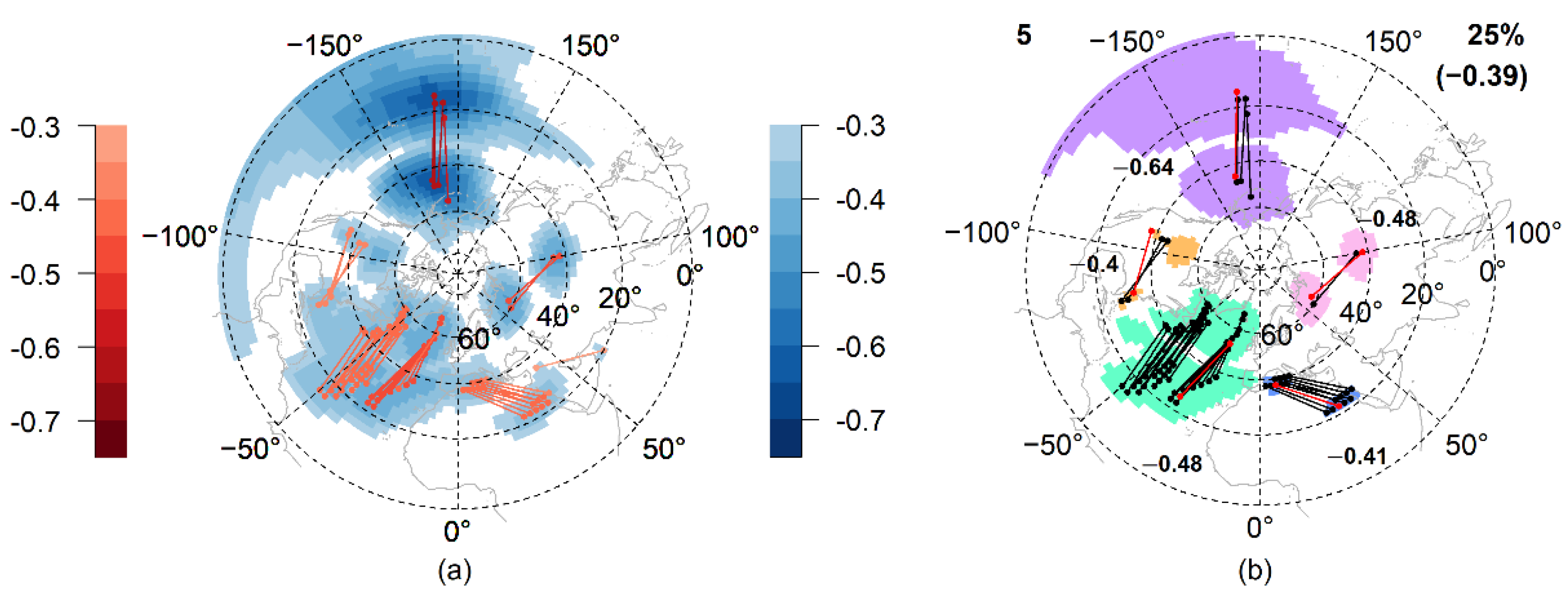
Figure 1.
(a) The fields of strongest negative correlations (SNC fields; blue-shaded grid cells) computed from the geopotential height field at the 500 hPa pressure level (zg500), for the period of 1976–2005. Potential action centers are denoted with red-shaded full circles connected with red-shaded lines. Brighter/darker colors indicate weaker/stronger correlations. (b) The map of cluster patterns obtained from the ERA-20C for the period of 1976–2005 (reference CP map) in accordance with [34] and Figure 2 therein. For the better visualization, clusters are denoted with different colors. The amount of the clusters is texted on the top-left corner of the map. Potential action centers are denoted with black dots connected with black lines, while the action centers are highlighted with red. The correlation associated with the action centers are texted on the map. The percentile and its associated correlation value can be seen in the top-right corner of the map in parentheses.

Figure 3.
The receiver operating characteristic (ROC) curves obtained from the GCM simulations under the RCP4.5 and the RCP8.5 scenarios, for the periods of 2006–2035, 2021–2050, and 2071–2100. The dashed straight lines represent the 45° line.
Figure 3.
The receiver operating characteristic (ROC) curves obtained from the GCM simulations under the RCP4.5 and the RCP8.5 scenarios, for the periods of 2006–2035, 2021–2050, and 2071–2100. The dashed straight lines represent the 45° line.

Figure 4.
The area under curve (AUC) values and the largest values of the Matthews correlation coefficient (MCCmax) (a) for the historical GCM simulations (data are provided in Table A1), (b) for the RCP4.5 simulations, and (c) for the RCP8.5 simulations (data are provided in Table 2). The GCMs are denoted with colored symbols in all the three plots. In (b,c) the symbols are replaced with numbers, where 1, 2, and 3 indicate the analyzed 30-year-long time periods. Black asterisks denote the mean values (in (a) AUC = 0.91, MCCmax = 0.56, in (b) AUC = 0.88, MCCmax = 0.58, in (c) AUC = 0.87, MCCmax = 0.58), while gray asterisks denote the median values (in (a) AUC = 0.91, MCCmax = 0.56, in (b) AUC = 0.87, MCCmax = 0.57, in (c) AUC = 0.88, MCCmax = 0.6).

Table 1.
The names and types (Earth System Model, ESM or Atmosphere-Ocean General Circulation Model, AOGCM) of the analyzed GCMs, the horizontal resolutions of the Atmospheric General Circulation Models (AGCMs), the institutes and the countries of their origins. The realizations r1i1p1 are used in all cases. The CMCC-CMS, the HadGEM2-CC, the IPSL-CM5A-MR, and the MPI-ESM-LR are GCMs with a well-resolved stratosphere.
| GCM | Type | Horizontal Resolution of the AGCM (Longitude × Latitude) | Institute and Country of Origin |
|---|---|---|---|
| ACCESS1-3 [37] | ESM | 1.9° × 1.3° | Commonwealth Scientific and Industrial Research Organization (CSIRO) and Bureau of Meteorology (BOM), Australia |
| CMCC-CM [38] | AOGCM | 0.8° × 0.8° | Centro Euro-Mediterraneo sui Cambiamenti Climatici (CMCC), Italy |
| CMCC-CMS [39] | AOGCM | 1.9° × 1.9° | Centro Euro-Mediterraneo sui Cambiamenti Climatici (CMCC), Italy |
| CNRM-CM5 [40] | ESM | 1.4° × 1.4° | Centre National de Recherches Météorologiques (CNRM), Météo-France, Centre Européen de Recherche et de Formation Avancée en Calcul Scientifique (CERFACS), France |
| HadGEM2-CC [41] | ESM | 1.9° × 1.3° | Met Office Hadley Centre (MOHC), UK |
| IPSL-CM5A-MR [42] | ESM | 2.5° × 1.3° | Institute Pierre-Simon Laplace (IPSL), France |
| MPI-ESM-LR [43,44] | ESM | 1.9° × 1.9° | Max Planck Institute for Meteorology (MPI), Germany |
Table 2.
The area under curve (AUC) values, the largest values of the Matthews correlation coefficient (MCCmax), and the associated percentiles obtained from the GCM simulations under the RCP4.5 and the RCP8.5 scenarios, for the periods of 2006–2035, 2021–2050, and 2071–2100. The reference CP map is obtained from the ERA-20C for the period of 1976–2005. The AUC and the MCCmax values, and the associated percentiles computed from the historical GCM simulations are shown in Table A1.
| GCM | Time Period | RCP4.5 | RCP8.5 | ||||
|---|---|---|---|---|---|---|---|
| AUC | MCCmax | Percentile (%) | AUC | MCCmax | Percentile (%) | ||
| ACCESS1-3 | 2006–2035 | 0.86 | 0.59 | 25 | 0.89 | 0.62 | 32.5 |
| 2021–2050 | 0.88 | 0.60 | 20 | 0.86 | 0.51 | 27.5 | |
| 2071–2100 | 0.83 | 0.50 | 20 | 0.81 | 0.50 | 15 | |
| CMCC-CM | 2006–2035 | 0.92 | 0.70 | 25 | 0.88 | 0.60 | 22.5 |
| 2021–2050 | 0.89 | 0.61 | 22.5 | 0.85 | 0.54 | 32.5 | |
| 2071–2100 | 0.88 | 0.60 | 30 | 0.89 | 0.62 | 25 | |
| CMCC-CMS | 2006–2035 | 0.89 | 0.61 | 30 | 0.88 | 0.54 | 20 |
| 2021–2050 | 0.87 | 0.54 | 22.5 | 0.88 | 0.60 | 25 | |
| 2071–2100 | 0.86 | 0.51 | 25 | 0.91 | 0.64 | 22.5 | |
| CNRM-CM5 | 2006–2035 | 0.88 | 0.61 | 20 | 0.90 | 0.67 | 25 |
| 2021–2050 | 0.85 | 0.56 | 27.5 | 0.89 | 0.61 | 30 | |
| 2071–2100 | 0.90 | 0.63 | 35 | 0.83 | 0.51 | 22.5 | |
| HadGEM2-CC | 2006–2035 | 0.93 | 0.69 | 25 | 0.91 | 0.69 | 25 |
| 2021–2050 | 0.89 | 0.63 | 22.5 | 0.91 | 0.65 | 25 | |
| 2071–2100 | 0.89 | 0.57 | 22.5 | 0.87 | 0.58 | 35 | |
| IPSL-CM5A-MR | 2006–2035 | 0.86 | 0.53 | 25 | 0.83 | 0.52 | 27.5 |
| 2021–2050 | 0.85 | 0.52 | 25 | 0.87 | 0.60 | 22.5 | |
| 2071–2100 | 0.85 | 0.50 | 20 | 0.80 | 0.64 | 30 | |
| MPI-ESM-LR | 2006–2035 | 0.87 | 0.56 | 27.5 | 0.88 | 0.51 | 27.5 |
| 2021–2050 | 0.87 | 0.54 | 35 | 0.84 | 0.47 | 32.5 | |
| 2071–2100 | 0.87 | 0.53 | 45 | 0.86 | 0.51 | 25 | |
Publisher’s Note: MDPI stays neutral with regard to jurisdictional claims in published maps and institutional affiliations. |
© 2022 by the author. Licensee MDPI, Basel, Switzerland. This article is an open access article distributed under the terms and conditions of the Creative Commons Attribution (CC BY) license (https://creativecommons.org/licenses/by/4.0/).
Share and Cite
MDPI and ACS Style
Kristóf, E. Evaluation of Future Simulations of the CMIP5 GCMs Concerning Boreal Wintertime Atmospheric Teleconnection Patterns. Meteorology 2022, 1, 450-467. https://doi.org/10.3390/meteorology1040028
AMA Style
Kristóf E. Evaluation of Future Simulations of the CMIP5 GCMs Concerning Boreal Wintertime Atmospheric Teleconnection Patterns. Meteorology. 2022; 1(4):450-467. https://doi.org/10.3390/meteorology1040028
Chicago/Turabian StyleKristóf, Erzsébet. 2022. "Evaluation of Future Simulations of the CMIP5 GCMs Concerning Boreal Wintertime Atmospheric Teleconnection Patterns" Meteorology 1, no. 4: 450-467. https://doi.org/10.3390/meteorology1040028