Article

Comparison of Methods to Segment Variable-Contrast XCT Images of Methane-Bearing Sand Using U-Nets Trained on Single Dataset Sub-Volumes

by
Fernando J. Alvarez-Borges
1,2,
Oliver N. F. King
2,*,
Bangalore N. Madhusudhan
1,
Thomas Connolley
2,
Mark Basham
3 and
Sharif I. Ahmed
2
1
Faculty of Engineering and Physical Sciences, University of Southampton, Southampton SO17 1BJ, UK
2
Diamond Light Source Ltd., Harwell Science & Innovation Campus, Didcot OX11 0DE, UK
3
The Rosalind Franklin Institute, Harwell Science & Innovation Campus, Didcot OX11 0QS, UK
*
Author to whom correspondence should be addressed.
Methane 2023, 2(1), 1-23; https://doi.org/10.3390/methane2010001
Submission received: 16 September 2022 / Revised: 28 October 2022 / Accepted: 5 December 2022 / Published: 20 December 2022

Abstract

:
Methane (CH4) hydrate dissociation and CH4 release are potential geohazards currently investigated using X-ray computed tomography (XCT). Image segmentation is an important data processing step for this type of research. However, it is often time consuming, computing resource-intensive, operator-dependent, and tailored for each XCT dataset due to differences in greyscale contrast. In this paper, an investigation is carried out using U-Nets, a class of Convolutional Neural Network, to segment synchrotron XCT images of CH4-bearing sand during hydrate formation, and extract porosity and CH4 gas saturation. Three U-Net deployments previously untried for this task are assessed: (1) a bespoke 3D hierarchical method, (2) a 2D multi-label, multi-axis method and (3) RootPainter, a 2D U-Net application with interactive corrections. U-Nets are trained using small, targeted hand-annotated datasets to reduce operator time. It was found that the segmentation accuracy of all three methods surpass mainstream watershed and thresholding techniques. Accuracy slightly reduces in low-contrast data, which affects volume fraction measurements, but errors are small compared with gravimetric methods. Moreover, U-Net models trained on low-contrast images can be used to segment higher-contrast datasets, without further training. This demonstrates model portability, which can expedite the segmentation of large datasets over short timespans.

1. Introduction

Deep sea sediments and perfmafrost host large quantities of methane (CH4), an energy source and potent greenhouse gas that may be a contributor to climate change [1,2]. Much of this CH4 is present as hydrates (clathrates), that is, solid crystalline lattices of water at low temperature and high pressures that enclose CH4 molecules. 164 m3 of CH4 gas at normal temperature and pressure can be stored in one m3 of hydrate [3]. However, the extent of the world-wide CH4 hydrate inventory is subject to considerable uncertainty [4,5]. This is in part due to discrepancies between measurements produced by geophysical and electrical resistivity methods [6,7]. These discrepancies are potentially associated with hydrate and CH4 gas distribution heterogeneity in the host soil [8]. Uncertainties regarding the global CH4 hydrate inventory affect resource estimation and CH4 emission prediction models [5,9,10]. CH4 hydrate formation and dissociation has also been associated with changes in the mechanical characteristics of the host sediment. For instance, hydrates may strengthen and stiffen the sediment matrix by creating inter-grain cementation bonds [11,12]. This is speculated to lead to, for example, underwater slides that may trigger tsunami or damage seabed infrastructure such as cables and pipelines [13,14,15].
Recently, researchers have shown that X-ray computed tomography (XCT) can be used to successfully detect hydrate and CH4 gas bubble distribution heterogeneity and characterise changes in sediment microstructure associated with hydrate formation and dissociation [8,16,17,18]. This has been possible in great part due to advancements in image segmentation techniques. Segmentation is the process of classifying 2D pixels or 3D voxels into regions, for example, the solids, liquids and gases present in XCT images of geomaterials. Microstructural parameters such as grain, pore and bubble size, shape and orientation can then be derived from the segmented image, as well as volumetric (bulk) quantities such as porosity and CH4 gas saturation ratios.
Some of the most common segmentation techniques used in geomechanics and geoscience are greyscale thresholding and watershed algorithms [19,20]. The former involves the selection of a greyscale range to classify pixels or voxels into regions of interest. Watershed algorithms redefine the image as a map where greyscale intensities form topographical elevations and catchment basins. Pixel/voxel markers within these basins are used to define the materials (or ‘labels’) present in the image, and the algorithm then morphologically dilates these markers until they fill their catchment basins [21,22]. Greyscale range determination in the case of thresholding techniques and marker grey value and location in the case of watershed techniques are operator and/or method dependent [19,23,24]. The values assigned to these parameters also depend on the recorded greyscale contrast, which is highly reliant on the X-ray imaging instrument and how it is optimised [25]. Sample heterogeneity or density changes during an in situ experiment will further introduce contrast variability in space and time [19,26]. As a result, thresholding and watershed segmentation are typically optimised per XCT scan, and objective comparison is difficult given that the data treatment varies between datasets. These issues often result in segmentation procedures in geomechanics and geoscience that are highly demanding of computing resources and operator time.
Novel alternative approaches have employed machine learning to segment multiple material phases present in XCT images of soil and rock samples [27,28]. For these applications, segmentations are produced via a mathematical model optimised or ‘trained’ using a series of ‘ground truth’ example segmentations of XCT images provided by the user. Within the realm of machine learning, convolutional neural networks (CNNs) are a class of deep neural networks that employ convolutional layers where the filters (‘kernels’) used to separate image features are learned [29]. Researchers have recently begun exploring the application of CNNs to segment XCT images of soil and rock [30,31,32,33].
U-Nets are a class of CNN originally designed to segment biomedical images [34]. The U-Net architecture is composed of downsampling (encoding/contracting) and upsampling (decoding/expanding) paths. The former reduces the spatial dimensions of the data while increasing feature information; the latter recombines spatial and feature data to generate the label image. Both paths are linked by connections that can feed the output from the contracting path directly into the corresponding level of the expanding path, thereby allowing the transfer of spatial information and the preservation of fine-grained details in the output label image. A limitation to the implementation of U-Nets (and CNNs in general) to segment XCT images of soil and rock is the preparation of training and validation datasets, which often require labour-intensive manual segmentation (hand-annotation) of many images.
The suitability of such time- and resource-saving approaches have not been examined before in research on methane-bearing sediments. This paper explores this application using three U-Net implementation strategies to segment a large number of synchrotron radiation XCT (SXCT) volumes of CH4-bearing sand during hydrate formation and dissociation experiments; two of these U-Net implementations are entirely novel to the field of geomechanics and geoscience. These strategies were focused on the segmentation of the CH4 phase, as it exhibited low contrast with regard to the brine-hydrate phase and was less common in the data compared to the other material phases, as shown in Figure 1a. This rendered the use of conventional thresholding or watershed techniques largely unsuitable. The aim of this investigation was thus to determine if U-Nets can accurately segment XCT images of soil samples with varying greyscale contrast between material phases using only a small number of training and validation images, therefore reducing operator and computing time and allowing for objective data comparison.
Section 2 of this paper presents the details of the in situ hydrate formation experiment as well as the methodology used to acquire, reconstruct and post-process the SXCT data. Section 3 describes the three U-Net approaches used, as well as the conventional segmentation methods and accuracy metrics used for comparison and performance analysis purposes. Results are presented and discussed in Section 3 and outcomes are summarised in Section 4.

2. Materials and Methods

2.1. Methane Gas Hydrate Formation and Dissociation Experiments

A custom rig designed and manufactured by Sahoo et al. [8] for in situ SXCT imaging of gas hydrate formation and dissociation was used in the present study. The rig is made of polyether ether ketone (PEEK) and consists of a monolithic 2 mm internal diameter by 23 mm tall cylindrical vessel with 0.8 mm thick walls and an enlarged base, as shown in Figure 2. The soil sample is placed through the bottom of the rig. The pore fluid injection pipe is connected to this inlet, as depicted in Figure 2. The rig features thermocouples at the base of the scan zone, shown in this Figure, to measure sample temperature. The SXCT imaging zone in this study corresponds to a vertically centred 1.755 mm-tall region within the 10 mm-tall scan zone.
Leighton Buzzard sand Fraction E (LBE) with mean grain diameter of 100 µm was used as surrogate marine sediment. LBE is an angular silica sand widely used as standard laboratory material in geomechanics research. The sand was tamped into PEEK vessel to a target porosity of 35%. A vacuum pressure of less than 1 Pa was applied through the injection pipe to reduce air presence in the pore space. A calculated volume of brine solution (3.5% NaCl by weight, representative of deep ocean water; [35]) was thereafter injected into the sample, such that approximately 90% of the pore volume became saturated. CH4 gas was then injected at 10 MPa and the valve to the sample closed. The sample was gradually cooled to a target constant temperature of 2 °C using a N2 cryostream. This thermobaric condition enabled hydrate formation in the pore space instead of ice. The target temperature was maintained for 30 h to complete the hydrate formation process [11].

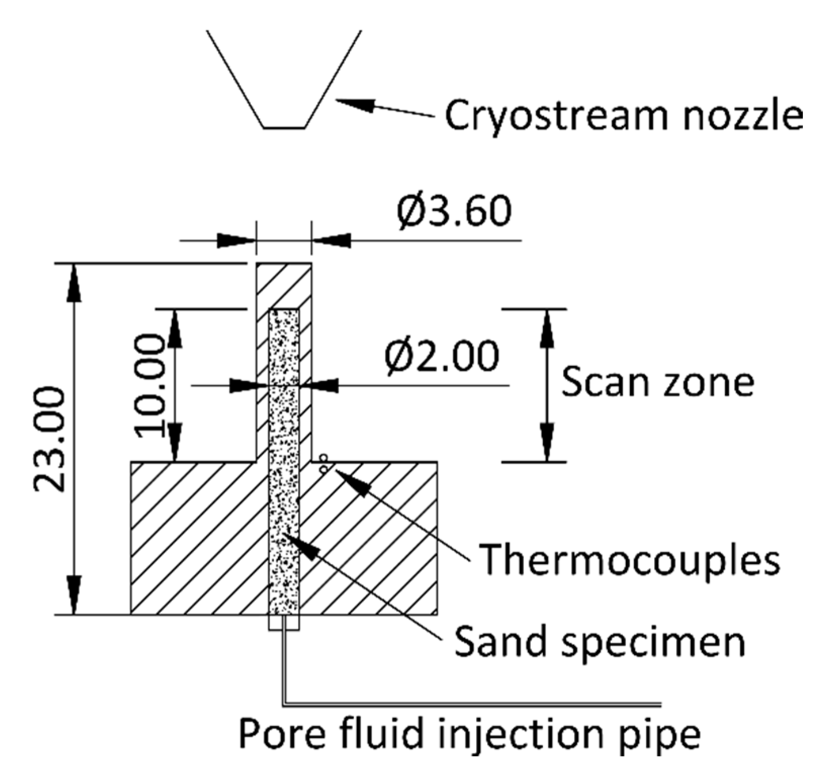
2.1.1. Set-Up and Image Acquisition

Data was collected on beamline I13-2 at Diamond Light Source (DLS). Scans were performed using a polychromatic ‘pink beam’ at 30 keV peak energy. The detector system used was a scintillator-coupled pco.edge 5.5 camera fitted with a 4× optic magnification lens, resulting in an effective pixel size of 0.8125 µm. The X-ray projection size was 2560 × 2160 pixels (width × height).
Scans were carried out in situ at various time intervals after reaching 2 °C. The number of projections and the exposure time per projection varied amongst scans to reduce acquisition times at specific moments of the CH4 hydrate formation process. Table 1 correlates each scan discussed in this paper with the time after the start of the 30 h sustained 2 °C period, as well as the scan specifications used.

2.1.2. Tomographic Reconstruction and Post-Processing

Tomographic reconstruction was carried out using Savu [36,37,38]. Two Savu reconstruction pipelines were used: one with and one without Paganin phase enhancement [39]. These pipelines were labelled ‘phase contrast’ (Figure 3b) and ‘absorption contrast’ (Figure 3a), respectively. Both pipelines implemented filtered back-projection reconstruction [40,41] and pre-reconstruction algorithms for speckle and ring artefact suppression [37,42] and the automatic determination of the centre of rotation [43]. Further processing was carried out on the output from both reconstruction pipelines using Fiji [44,45]. This consisted in:
  • The application of a median filter of kernel size 3 to the absorption volume and the halving of the resulting greyscale values;
  • The application of an unsharp mask filter of radius 3 and weight 0.70 to the phase contrast volume;
  • The elementwise averaging of both volumes.
This procedure resulted in a single reconstructed volume with clear edge detail and phase contrast (Figure 3c).
Finally, to mitigate the halo-like or ‘cupping’ artefact caused by the preferential attenuation of lower-energy X-rays close to the specimen surface, known as beam hardening, as well as by truncation artefacts introduced by attenuation from sample regions outside the field of view [46,47]), each slice was convolved with two mollifier functions with an inverse shape to that of the cupping artefact. This flattened the horizontal (XY) grey value profile of each slice. A circular mask with a radius of 1100 pixels was then applied to remove voxels at the outer edges of the field of view (FOV), which were resistant to cupping correction. An example output slice is presented in Figure 3d.
As outlined in Section 1, limited greyscale contrast between the CH4 gas and the brine-hydrate phase persisted after reconstruction and post-processing. Distinction between these two phases became increasingly difficult as the distance between the 3D image histogram peaks for the sand and non-sand phases reduced, as exemplified in Figure 1b. This distance is therefore used in this paper as an overall measure for image contrast, with regard to the ease with which the material phases could be identified and segmented. Considering this, intermediate contrast dataset IC01 89062 (Table 1) was selected initially to investigate the suitability of U-Nets to perform segmentations.

2.2. U-Net Segmentation

Three different methodologies were used to create trained U-Net models to segment the three main material phases present in the images: sand, brine-hydrates and CH4 gas. These were:
  • A 3D hierarchical approach where two separate 3D U-Net models were trained to perform binary segmentations: On the sand phase vs. the others and the CH4 gas phase vs. the others;
  • A 2D multi-label and multi-axis approach where a single 2D U-Net was trained to classify the three labels. The encoder section of this U-Net implementation was pre-trained on the ImageNet dataset [48], meaning that the network should only require a small amount of ‘transfer’ training in order to achieve acceptable results on new data;
  • RootPainter software, which uses a graphical user interface (GUI) and human intervention by interactive corrections to train a lightweight binary 2D U-Net model.
The U-Net models produced by each method were used to segment a 1554 × 1554 × 2000 voxels sized region of the 2560 × 2560 × 2000 voxels sized reconstructed and post-processed volumes, hereafter termed ‘analysis region’ and ‘total volume’. The analysis region was inscribed within the cylindrical FOV of the total volume and omitted the black pseudo-background generated during reconstruction. Figure 4a shows the analysis region for dataset IC01. All analysis regions discussed in this paper are available in Alvarez-Borges et al. [49]. It is emphasised that the segmentation of the sand phase via U-Nets was done to assess the multi-label segmentation capacity of the algorithm. Due to its uniformly high-contrast and well-defined edges, sand could be easily segmented with any ‘conventional’ method, for example, thresholding.

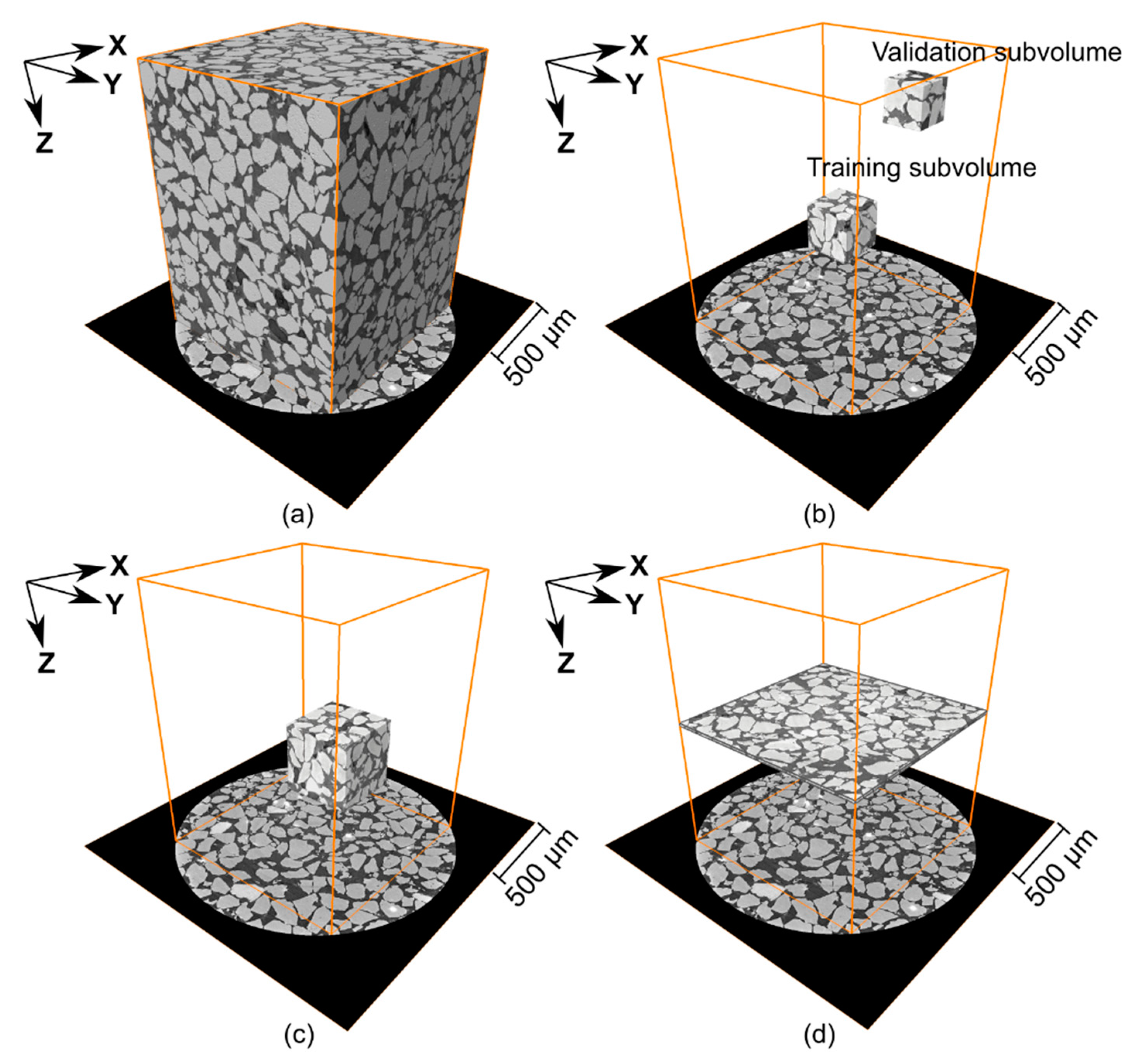
2.2.1. Training and Validation Data

The U-Net training procedures required both greyscale and label datasets. The latter was the ‘ground truth’ information used during training and validation. Label data was produced by hand-annotating the sand, CH4 gas and brine-hydrate in the greyscale data using Avizo Lite® software. This was carried out on small subregions of the analysis volumes to reduce labelling time. The 3D hierarchical approach initially used a 384 × 384 × 384 voxels sized training subvolume and a 256 × 256 × 256 voxels sized validation subvolume, selected from two different regions of the 3D image (Figure 4b). These are hereafter referred to as 3D training and 3D validation subvolumes, respectively. RootPainter requires 2D label images (slices) of at least 572 × 572 pixels in size for both training and validation, as explained later in Section 2.2.4. Therefore, a 572 × 572 × 572 voxels sized subvolume was delimited for this purpose (Figure 4c), hereafter referred to as 2D learning subvolume. The same 2D learning subvolume was used only to train the 2D multi-label models, with the 3D validation subvolume used for validation as with the 3D methods.
The 2D and 3D training and validation subvolume coordinate origins relative to the global origin of the total volume are listed in Table 2 (note in column three that all subvolumes were 3D arrays, despite their naming and usage). The global coordinate system origin is indicated in Figure 4. All training, validation and segmented data used in this investigation are available in [49].

2.2.2. 3D Hierarchical Segmentation

The 3D hierarchical U-Net model was implemented in the Python library PyTorch [50] and based upon an existing implementation of a residual 3D U-Net from the literature [51,52]. This model had 35.3 million trainable parameters and five downsampling and upsampling stages. Voxel intensity values were rescaled and clipped, truncating values beyond 2.575 standard deviations of the mean to mitigate the skewing effect of outliers. The ground truth label volumes (3D training subvolume with three labels: sand, brine-hydrates and CH4 gas) were used to create separate binary label volumes, one with sand vs. background and the other with CH4 gas vs. background. These volumes were used as the label data for training the separate binary 3D U-Net models.
Unlike the multilabel 2D U-Net implementation described later, this model had not been pre-trained on ImageNet and was therefore likely to require a larger amount of training data to reach a high segmentation accuracy. To overcome this, the TorchIO library [53] was used to sample 128 × 128 × 128 voxels sized regions from the greyscale 3D training subvolume and generate 48 sets with random noise, flips, blurs, affine, and elastic transformations to be used as an extended training data set for each training epoch (i.e., a full training cycle). This procedure is termed ‘augmentation’. These 128 × 128 × 128 voxels regions matched the input size of the U-Net.
During training, U-Net model parameter optimisation (i.e., the process of updating the model parameters on each training iteration) was carried out with a method known as AdamW [54]. The learning rate, a parameter that controls the step size of the updates made by the optimiser, was initially determined automatically and then cycled up and down every epoch to reduce the need to tune this parameter and to accelerate the training process [55]. The parameters β1, β2 and weight decay were set at 0.9, 0.999 and 0.1, respectively. Binary cross entropy (BCE), a measure of the uncertainty between two data distributions, was used as the loss function (the function minimised by the optimiser during training). Training progress was monitored using Intersection Over Union (IOU) on the validation set as the evaluation metric. If either no improvement in validation loss occurred after 40 passes of the entire training dataset (epochs) or 100 epochs were completed, the model with the lowest validation loss was saved. This was aimed at preventing overfitting. Software source code for this method is available from King and Alvarez-Borges [56].
When predicting the segmentation of the analysis region, two binary predictions were produced for each data set, one for sand vs. background and the other for CH4 gas vs. background. These two label volumes were then combined using a label hierarchy: first, a new volume was created with all voxel labels set to brine-hydrates, then the labels corresponding to CH4 gas were transferred from the CH4 vs. background prediction, and lastly the labels corresponding to sand were transferred from the sand vs. background prediction.

2.2.3. 2D Multi-Label Segmentation

Training of the 2D U-Net with multiple labels was performed using the 2D learningsubvolume using two approaches. The first mimicked that of RootPainter, described later, with the network being trained on horizontal 2D (XY) slices through the image volume. The second, multi-axis approach, utilised slices taken in the XY, XZ and YZ planes (coordinate system shown in Figure 4). A 2D U-Net was used with a ResNet34 encoder [57]. This model had a total of 41.2 million trainable parameters and four downsampling and upsampling stages. This encoder was loaded with pre-trained weights from ImageNet. The model was created with Fastai [58], a Python library which has a high-level interface that utilizes PyTorch. Default Fastai image augmentations were used during training. These consisted of random image crops, zooms, rotations, flips, affine transforms and brightness and contrast adjustments. The loss function used was cross entropy (CE) and the evaluation metric used was the number of correctly labelled voxels expressed as a percentage. Training was carried out for 15 epochs.
For the single-axis implementation, the XY greyscale stack and corresponding label stack of 572 images were randomly split into training (80%) and validation (20%) sets. The input image size for the model was also set to 572 × 572 pixels to match that used by RootPainter. When predicting the segmentation for the analysis region, data was fed into the network in the form of 2000 XY slices of size 1554 × 1554 pixels.
For the multi-axis approach, the 2D greyscale learning subvolume and corresponding label data were sliced into 2D images in the XY, XZ and YZ planes, resulting in 1716 (572 × 3) training image and label pairs. These images were also randomly split into a training (80%) and validation (20%) set. The input image size for the model was again set to 572 × 572 pixels. When predicting the segmentations for the analysis region, an averaging approach for data produced from each plane was used as described by Tun et al. [59], but with a modification to take the multiple labels into account. In short, this averaging approach consisted in slicing, segmenting, and rotating the volume across the XY 4-fold symmetry plane and then splitting and hierarchically recombining the 12 resulting segmentation volumes so that two label volumes were obtained, one containing labels for sand vs. background and the other for CH4 vs. background. These two binary label volumes were then combined into a multi-label volume as done for the data output from the 3D hierarchical method (Section 2.2.2).
Software source code for this method is available from King and Alvarez-Borges [56].

2.2.4. RootPainter Segmentation

RootPainter [60] is a client-server application originally developed to segment plant root features from photographs of soil profiles [61,62]. The client GUI is employed to annotate 2D images from a dataset, such as a tomography image stack of horizontal (XY) slices, as in the present case. The tomography slices and corresponding annotations are then read by the server and used to train the segmentation model using a U-Net variant with 1.3 million trainable parameters and four downsampling and upsampling stages. This is implemented in PyTorch and described by Smith et al. [61] and Smith et al. [62]. To execute the training routine, the software creates a validation dataset by randomly selecting one annotation image out of every five created. The accuracy of the model produced at the end of each training epoch is evaluated using the F-score parameter described by Smith et al. [62]. At the end of each training epoch, F-score values for the current and previous model are compared and the one with the highest value is saved. Training is stopped if 60 epochs are completed without F-score improvements.
RootPainter uses interactive corrections. These are created by annotating image slices overlaid with the segmentation labels produced by the best model currently available. These corrective annotation slices are added to the training and validation datasets so that the five to one ratio is maintained.
RootPainter 0.2.5 can only predict binary segmentations (‘foreground’ vs. ‘background’). Therefore, it was initially used to segment the CH4 gas phase only. The 2D learning sub-volume was used for training and validation.
Sparse annotations have been shown to produce better results than dense/intensive annotations when interactively training U-Net models [61,63]. Thus, arbitrarily sparsely annotated images were produced by converting all CH4 gas labels into foreground and enclosing them with background labels that included brine-hydrate and sand pixels, as shown in Figure 5a,b. This was done by morphologically dilating the CH4 label of each slice in the training dataset and re-labelling the added pixels as background. The annotated slices were then copied into annotation and validation directories, maintaining the five-to-one ratio. Training was initiated after copying the first batch of five images. Further batches were added if a training epoch finished without further improvements in F-score and the model could not segment the majority of CH4 pixels, or if the erroneously segmented pixels were patently greater than the number of correctly segmented pixels, as shown in Figure 5c. Corrective annotation was started after a training epoch had produced a model that segmented most of the CH4 regions with a roughly equivalent number of erroneously labelled pixels, as presented in Figure 5d,e. Once a model was produced that could segment CH4 without evident erroneously labelled pixels, the software was left to carry on training until the 60-epoch limit was reached. The resulting model was then used to segment the analysis region slice by slice.

2.3. Thresholding and Watershed Segmentation

To compare the performance of the U-Net methods with conventional segmentation routines, the SXCT data was segmented using manual and automatic thresholding, and the watershed method. Images were downsampled to 8-bit as in the U-Net methods described previously. A bilateral filter was used before segmentation to improve thresholding performance and mitigate over-segmentation (filter parameters were:100-pixel spatial kernel, 50-pixel window size, and a grey-value kernel of 30 counts; implemented in Python using the open-cv library, Bradski [64]; see, e.g., Paris et al. [65] for filter description).
Manual thresholding was carried out by selecting a single threshold value for all slices by visual inspection. Automatic thresholding was performed on a slice-by-slice basis using the multi-level Otsu method [66] implemented using the scikit-image Python library [67].
Watershed segmentation was carried out in Fiji using the morphological segmentation tool in the Morpholibj library [68]. It consisted in the application of a morphological gradient with radius of 1 and the automatic determination of markers by finding local minima (with a tolerance of 8 greyscale intensity values), prior to the watershed ‘inundation’ phase. The output label image contained different labels for all features in the greyscale input image, including sand and brine-hydrate. Labels corresponding to regions in the 8-bit volume with mean greyscale intensity values below 50 to 70, depending on the dataset, and above 130 were classified as CH4 gas and sand, respectively. The remaining voxels were classified as brine-hydrates.

2.4. Quantitative Analysis

The central 40 XY slices of the segmented analysis region were compared with hand-annotated counterparts created in Avizo Lite® and considered to represent ‘ground truth’ labels. These slices do not intersect any of the training or validation subvolumes. These ground truth volumes are available in Alvarez-Borges et al. [49]. The previously mentioned IOU metric was used to evaluate segmentation performance. IOU is defined as:
IOU = TP TP + FN + FP ,
where TP refers to the number of voxels or pixels correctly predicted to correspond to the label of interest (‘true positive’), and FP and FN are the number of voxels or pixels incorrectly predicted to be part of the label of interest (‘false positive’) and voxels/pixels incorrectly predicted to belong to any of the other material phases (‘false negative’), in each case. A comparable analysis of U-Net accuracy has been done by, e.g., Karabağ et al. [69] and Phan et al. [32].
IOU returns a value between 0 and 1, where the latter corresponds to the scenario were the segmentation matches the validation image pixel by pixel (or voxel by voxel). In the following sections, quantitative analyses were carried out on a slice-by-slice basis (i.e., using pixel counts as input).

3. Results and Discussion

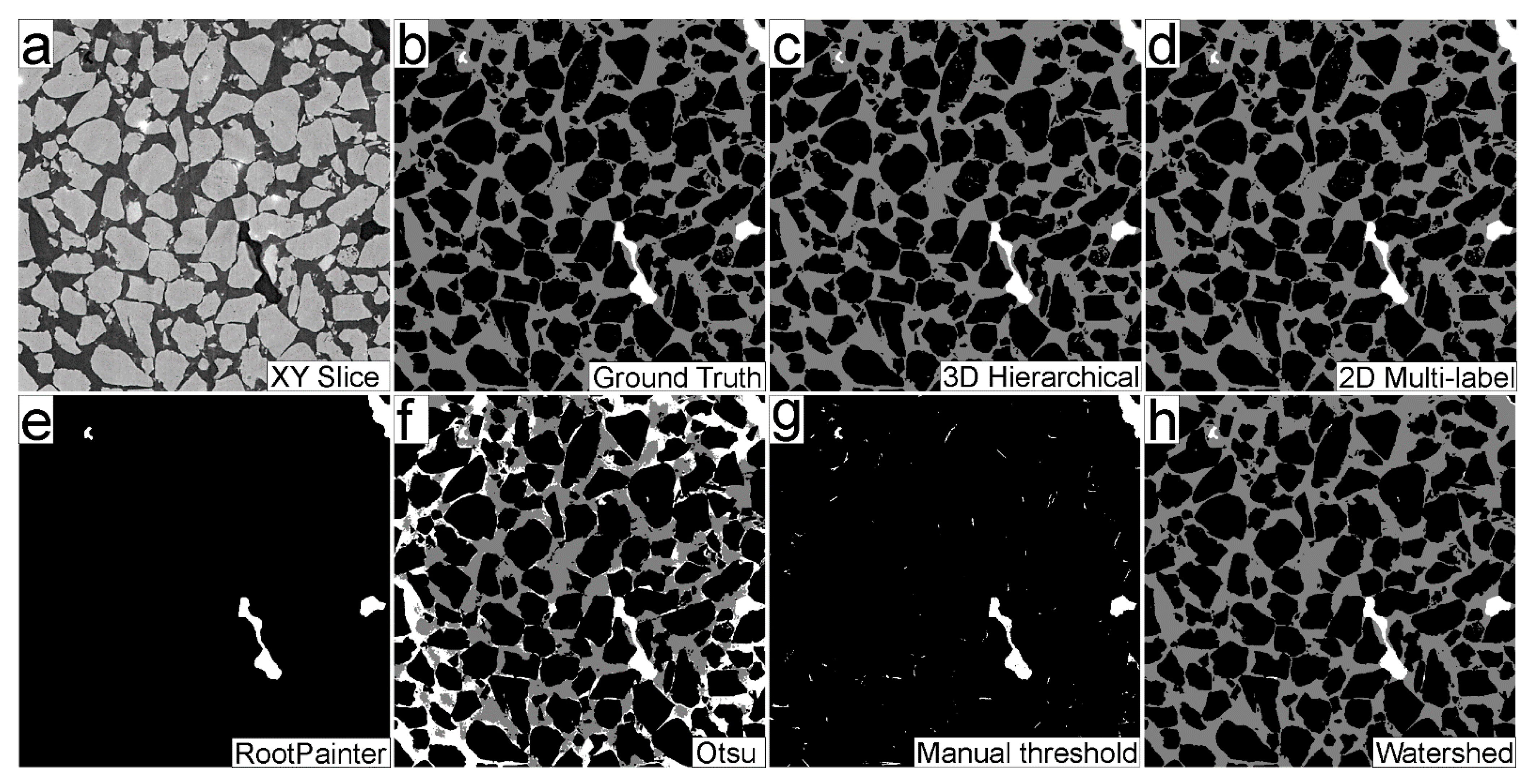
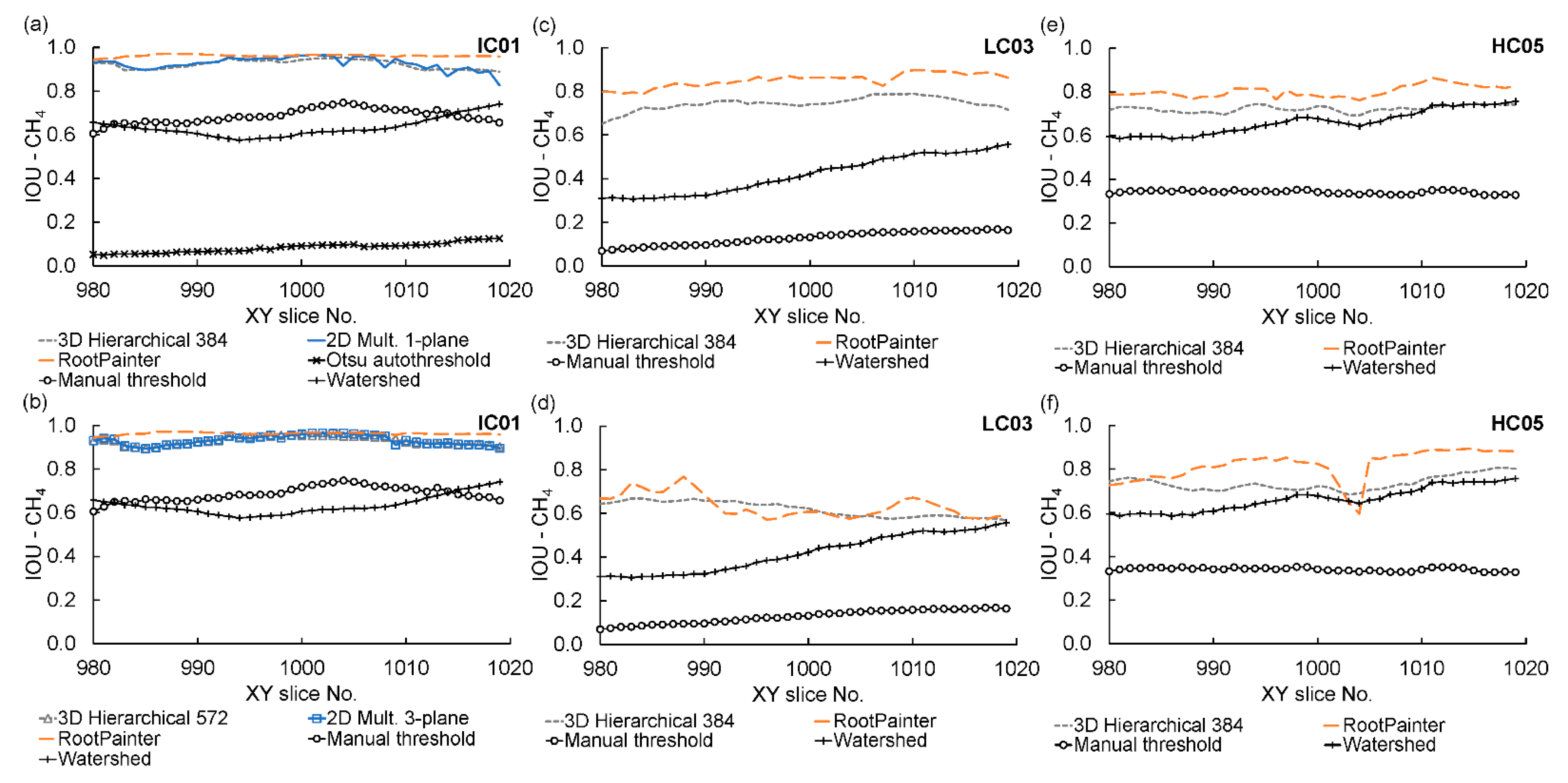
3.1. Segmentation Performance Comparison

Figure 6 compares the original and segmented central slice for dataset IC01, produced using the three U-Net methods (Section 2.2) and three standard methods (Section 2.3). Training and validation in both the 2D multi-label approach and RootPainter was carried out using XY slices only (i.e., single plane). Figure 7a presents accuracy metrics for the segmentation of CH4 gas in the central 40 XY slices this dataset. It may be noted that RootPainter delivered slightly higher metrics than the other two U-Net methods, but this difference in performance cannot be readily identified in Figure 6. Figure 6 and Figure 7a also show that, for this dataset, watershed and manual thresholding methods return lower accuracy results than the U-Net approaches, and that Otsu-thresholding performed poorly. In fact, the Otsu approach consistently segmented the brine-hydrate and CH4 gas as a single label, as evident in Figure 6e. This is chiefly due to the absence of well-defined inter-class variance extrema between these materials and the small relative size of CH4 bubbles [70,71]. In later comparisons, results from the Otsu method are omitted for this reason.
Since each model had been trained to convergence with their respective data, the slightly lower performance metrics observed in Figure 7a for the 3D hierarchical output, compared to that of RootPainter, may be attributed to the smaller training subvolume used. To present a more balanced comparison, a further 3D hierarchical model was trained on a subvolume of the same size as the one used for both 2D methods, i.e., the larger 2D learning subvolume. This comparison is presented in Figure 7b, where it is evident that RootPainter still outperformed the 3D hierarchical approach, though the difference between methods reduced. While an even larger training subset may deliver more substantial improvement, the preparation of such data would require much greater operator input, which is contrary to the aim of this study.
Figure 7a,b show that pre-training on the ImageNet database for the 2D multi-label method did not result in a significant segmentation performance advantage over the 3D hierarchical method. A similar outcome on the effect of transfer learning has been reported by He et al. [72]. They remarked that, ultimately, pre-training primes the U-Net for feature identification, which leads to fewer training iterations rather than greater segmentation accuracy. Such appears to be the present case, as the 2D multi-label approach produced similar results to the 3D hierarchical method with up to six times fewer training epochs, as shown in Table 3 and Table 4.
A disadvantage of the use of 2D U-Net segmentation methods that operate solely with XY slices, such as RootPainter and the single-axis 2D multi-label method, is that horizontal stripe artefacts may appear in the vertical (YZ or XY) slices of the segmented volume. This occurs because training and segmentation does not account for feature continuity between slices. Such artefacts are absent in the output of the 3D hierarchical implementation, which is reflected in the “smoothness” of the line showing the per-slice metrics for this approach in Figure 7. These artefacts can be mitigated by predicting segmentation of data slices taken along different axes and subsequently recombining them into a single volume, as done for the multi-axis 2D method, described in Section 2.2.3. This also improves the algorithm segmentation performance metrics, as shown in Figure 7b, but at the expense of greater computation times, as presented in Figure 8.

3.2. U-Net Performance on Data with Different Greyscale Contrast

The trained U-Net models created with all three methods described above were able to predict high-quality segmentations for the intermediate contrast dataset IC01 when trained on subsections of the same dataset. To examine if similar results could be obtained on datasets exhibiting lower greyscale contrast, both 3D hierarchical and RootPainter U-Nets were used to segment ‘low’ contrast dataset LC03 (Table 1, Figure 1b), using 3D training and 2D learning subvolumes of the same data for training, respectively. Figure 7c presents the performance metrics resulting from this approach, as well as those of watershed and manual thresholding methods applied to the same volume. It may be noted that both U-Net methods return lower metrics than those used on IC01. The IOU computations show that, on average, 74% and 85% of the voxels predicted to be CH4 gas were true positives in the 3D hierarchical and RootPainter results, respectively. In comparison, these average values were 92 and 94% for IC01.
Figure 9a shows that, for both U-Net methods, the lower performance metrics of the segmentation for LC03 are driven by false positives. However, false positives are over twice as numerous than false negatives in the results for the 3D hierarchical approach, whereas they only surpass false negatives by about 30% in the RootPainter segmentation. For both methods, most false positives correspond to ground truth brine-hydrate voxels incorrectly labelled as CH4 gas, as depicted in Figure 9b. This indicates that the reduced grey value differentiation (i.e., contrast) between CH4 gas and brine-hydrate phases restricted U-Net segmentation accuracy, as anticipated. Despite this, the U-Net methods significantly out-perform the standard approaches, as shown in Figure 7c. In fact, performance numbers reveal that watershed and manual thresholding cannot deliver a reliable quantification of the material phases of this low contrast dataset.

3.3. U-Net Segmentation Model Generalisation across Datasets (Model Portability)

To examine U-Net model portability, ‘low’ and ‘high’ contrast datasets LC03 and HC05 (Table 1, Figure 1b) were segmented using the models produced from training on ‘intermediate’ contrast dataset IC01. Figure 7d,e presents the performance metrics of the resulting segmentations. It can be observed that segmentation accuracy is lowest in the case where the U-Net models trained on mid-contrast dataset IC02 were applied to the low-contrast dataset LC03. IOU values from this process are comparable to those obtained from the thresholding and watershed methods applied to mid-contrast dataset IC01, and thus, quantification from these segmentations may be unreliable. The U-Net model trained on IC01 produced higher accuracy segmentations of high-contrast dataset HC05, comparable to those for the segmentation of low-contrast dataset LC03 using models trained ‘natively’ on LC03 subvolumes. Yet, it is evident that U-Net models trained on subvolumes of IC01 perform best when applied to the same ‘native’ IC01 dataset, as shown by Figure 7a,e.
As segmentation performance appeared to be higher when U-Net models trained on lower contrast data were used to segment higher contrast data, models trained on low-contrast LC03 images were used to segment high-contrast dataset HC05. Performance metrics are presented in Figure 7f. This Figure shows an overall improvement in performance metrics compared with segmentations produced with the U-Net models trained on IC01 (Figure 7e). However, an instance of localised poor performance for RootPainter can be observed in the profiles of Figure 7f, which resulted from a cluster of FP pixels on a single slice. This emphasises the limitations of the slice-by-slice (2D) segmentation described in Section 3.1, and denotes a broadly similar pattern of FP-driven model inaccuracy as for the results discussed previously in Section 3.2 (Figure 9).

3.4. Applications and Implications

The segmentation of XCT or SXCT images of soil and rock samples is often carried out to determine parameters such as porosity or liquid/gas saturation, as discussed in Section 1. The varying performances of the U-Net methods used in the present investigation result in differences in the parameters calculated from the segmented images. This is exemplified in Figure 10, which compares porosity and CH4 gas saturation (by volume) ratios derived on a slice-by-slice basis from the segmented volumes produced with the 3D hierarchical approach (3D training sub-volume) and RootPainter, which were the procedures that seemed to provide the best results with the least user time. Calculation details are provided in Appendix A.
Results presented in Figure 10 correspond to two application scenarios, that is:
  • U-Nets trained on sub-volumes of the dataset of interest are then used to segment the entire dataset, shown in Figure 10a,d. As discussed in Section 3.2, differences in greyscale contrast affect the performance of the resulting segmentation. A training sub-volume needs to be created for each scan;
  • U-Nets trained on sub-volumes of a low-greyscale contrast dataset are then used to segment other ‘unknown’ datasets of higher greyscale contrast (model portability). This is presented in Figure 10e,f, corresponding to parameters derived for high-contrast dataset HC05 using segmentations produced from U-Nets trained on sub-volumes of low-contrast dataset LC03. Thus, only one training sub-volume is needed to segment multiple scans.
Porosity and CH4 saturation calculations derived from manual thresholding and watershed methods are also included in Figure 10. This Figure suggests that, while U-Net models trained on a sub-volume of the same data delivered high segmentation performance metrics for the CH4 gas phase, the derived parameters deviated from ground truth values to some extent, this being more acute for porosity inferences. In fact, in most cases watershed or thresholding methods delivered more accurate porosity profiles. A comparison between the mean absolute error (MAE) for the porosity and CH4 saturation calculations along with the mean IOU values for the combined CH4 gas and sand labels from the three volumes used to generate Figure 10 is shown in Figure 11. This Figure reveals that, while there is a general trend of lower MAE for derived material parameters with higher segmentation accuracy, the correlation exhibits some scatter. Considering that both CH4 gas saturation and porosity are in part derived using the number of sand voxels and that these are significantly more numerous than pore voxels (CH4 gas and brine-hydrates), it may be proposed that errors in porosity/CH4-saturation estimation originate from inaccuracies in the segmentation of the sand phase. This is evidenced in Figure 12 for dataset IC01, which presents (a) IOU metrics for the segmentation of the sand phase and (b) the number of FP and FN voxels. Figure 12a reveals that the inaccuracies in the segmentation of the sand phase are relatively small in terms of metrics, which are in fact higher than those of the CH4 gas phase presented in Figure 7a. However, Figure 12b shows that the number of FP and FN voxels is large compared to the size of the CH4 gas and brine-hydrate phases, which amount to roughly 3.0 × 10⁴ and 8.75 × 10⁵ voxels per slice, respectively. This, in turn, affects parameters calculated from voxel counts. This denotes that the estimation of soil parameters based on ratios between material phases from segmented images is particularly sensitive to the relative size of said phases. It should be noted, however, that the maximum absolute errors presented in Figure 11 for U-Net-derived parameters (1.40% and 0.26% for porosity and CH4 gas saturation, respectively) are smaller than those commonly reported for laboratory methods [73,74,75].
Figure 12a also shows that thresholding and watershed methods are very effective at segmenting abundant, high-contrast, well-defined features like sand, as stated in Section 2.2. Indeed, the use of U-Nets may not be necessary or recommended if only such segmentations are required, as mentioned in Section 2.1.2. However, mainstream methods return unsatisfactory CH4 gas saturation measurements, particularly for the low-contrast 89069 volume, as shown in Figure 10. This is due to their inability to detect scarce, low-contrast features like CH4 bubbles, as demonstrated in Section 3.1.
A further application for U-Net segmentations of XCT/SXCT images of soil and rock is 3D data visualisation, which can then be used to investigate, for instance, CH4 gas distribution within the pore matrix. Such application can greatly benefit from model portability. To exemplify this, Figure 13 compares 3D views of the CH4 gas phase produced by segmenting datasets obtained at different stages of hydrate formation (Table 1) using the RootPainter model trained on the low-contrast LC03 sub-volume. Despite the presence of a modest number of segmentation errors in the form of small islands on some of the images (Figure 13b–d), the U-Net model produces sensible 3D representations of the data, and changes in CH4 gas distribution as it is consumed for hydrate formation can be clearly distinguished. In a further example, a 2D multi-label U-Net, trained using the single-axis approach on the 2D learning subvolume from scan IC01, has been used to segment a higher-contrast SXCT scan from a similar experiment carried out at the Swiss Light Source (SLS) originally reported by Sahoo et al. [8]. The post-processing steps described in Section 2.1.2, except cupping correction, were applied to the reconstructed data and a 1554 × 1554 × 2000 voxel region was extracted from the centre of the 3D image (data is available from Alvarez-Borges et al. [49]). Results are shown in Figure 14, where it is seen that the model delivers qualitatively accurate 3D views of the distribution of all three material phases, without any additional training, corrections or user input.
Both examples demonstrate the capability of U-Net models to segment multiple SXCT images of CH4-bearing soil, despite being obtained using different instruments and set-ups. The U-Net models used only a single (572)3 voxel sub-volume for training and did not require any additional training, corrections or user input to segment new images. A key implication is that training of a single U-Net model on a low greyscale contrast dataset could be used to deliver insight on variations in sediment morphology in other datasets. This has valuable applications. For example, segmentations are often required during a short period of time with limited operator input, such as during data acquisition at a synchrotron or other X-ray facility. The availability of pre-trained U-Net models would allow segmentations and sediment morphology/microstructure information to be produced within a short time after acquisition and reconstruction. Pre-trained models could also be used to segment numerous and/or large data sets over shorter timespans with reduced user effort and bias. However, accuracy will remain lower that what could be obtained with a model trained ‘natively’ on a subset of the target SXCT volume.
Future work could encompass, for instance, an analysis of the effect of U-Net segmentation accuracy and training strategy on ‘second order’ metrics such as particle, pore and bubble morphometry, as well as the potential for improving a model’s ability to generalise and accurately segment new data by including training data from several SXCT volumes with varying contrast characteristics.

4. Conclusions

The application of U-Nets to segment SXCT images of CH4-bearing sand has been investigated. The general aim was to determine if these convolutional deep learning networks, trained on a small set of images (≤(572)3 voxels), were capable of accurately segmenting large SXCT datasets (2000 × (1554)2 voxels) of different greyscale contrast, with focus on the CH4 gas phase. Training images were obtained from a hand-annotated subset of the reconstructed SXCT data. Three U-Net deployment methods were used: 3D hierarchical, 2D multi-label and the RootPainter application. Quantitative comparisons amongst U-Net segmentation outputs, along with mainstream thresholding and watershed methods, were carried out using the IOU metric. Major outcomes of this investigation are presented below.
  • For a given SXCT data set, the three U-Net deployment methodologies produced models capable of delivering segmented images of the CH4 gas phase with average IOU metrics of at least 0.74 and up to 0.93. This demonstrated that the U-Net methods used were capable of accurately identifying the CH4 gas phase using a small number of training images. RootPainter delivered marginally higher IOU metrics than the other methods but suffered from minor horizontal stripping artefacts and required more human intervention and proportionally higher computing time;
  • Greyscale contrast between material phases in the different SRXCT datasets was a significant factor affecting U-Net segmentation accuracy. The lowest segmentation performance metrics corresponded to SRXCT datasets exhibiting the lowest greyscale contrast, while greater segmentation accuracy resulted from the use of higher contrast data;
  • All U-Net segmentations of CH4 gas outperformed thresholding and watershed methods. However, mainstream methods proved to be more accurate at segmenting abundant, well-defined, and high-contrast features, like sand. U-Net methods are, thus, not recommended for this task;
  • The ability of a U-Net model trained on a subset of one dataset to generalise and produce an accurate segmentation of a different dataset, was explored. It was found that models trained on lower-contrast images were able to produce accurate segmentations of higher-contrast data without additional training. In comparison, U-Net models trained on higher-contrast images were found to deliver poor results when used to segment lower-contrast data. ‘Portability’ was further demonstrated by accurately segmenting independent data from a different synchrotron facility without additional training. This suggests that targeted training on small amounts of ‘ground truth’ data can produce U-Net segmentation models that can be used for rapid segmentation of a large number of different datasets with additional user input or training. However, segmentation accuracy will be lower than that of a model ‘natively’ trained on subsets of the target dataset;
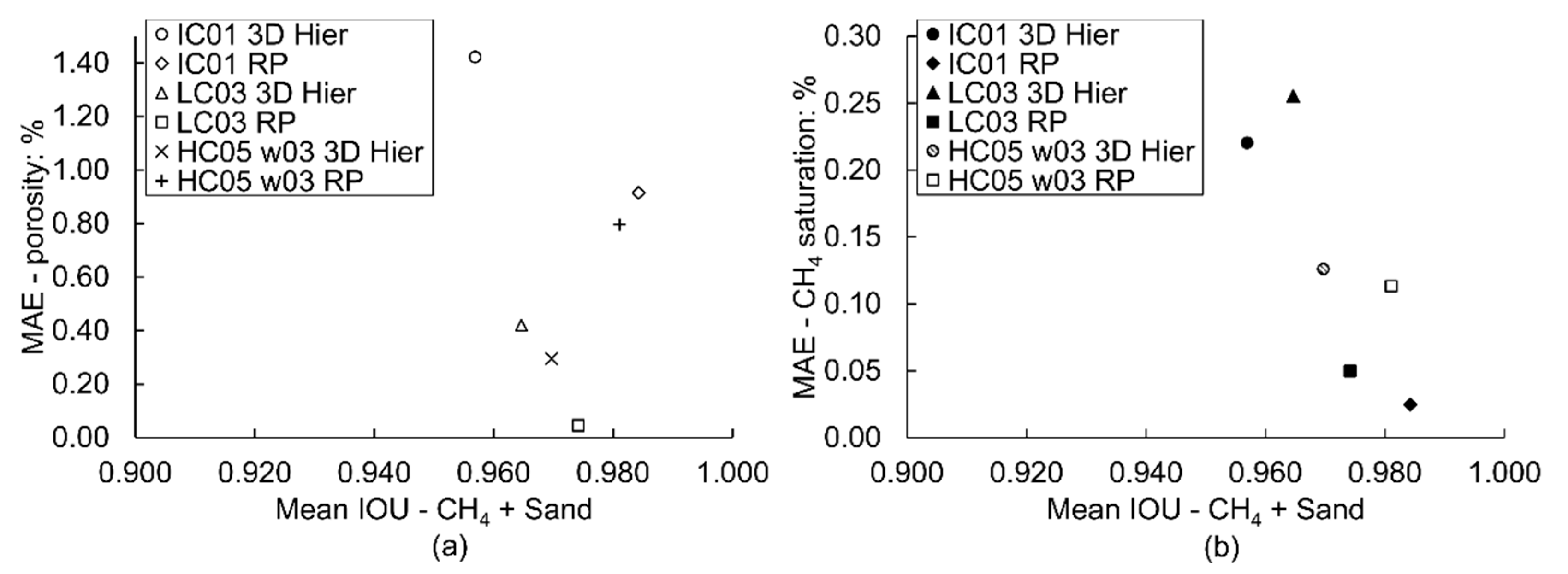
  • The effect of segmentation accuracy on image-derived material parameters was investigated by calculating porosity and CH4 gas saturation profiles using U-Net segmentations. A general trend of lower mean absolute error of the derived parameter with greater segmentation accuracy was found, but the correlation exhibited some scatter. Considering that porosity, fluid saturation and other parameters are ratios between material phases, it was proposed that errors in derived parameters are not only linked to segmentation accuracy metrics but to the number of false positive and negative voxel labels of the largest phase relative to the other phases.

Author Contributions

Conceptualisation, O.N.F.K., F.J.A.-B. and S.I.A.; methodology, O.N.F.K., F.J.A.-B., S.I.A. and B.N.M.; software, O.N.F.K.; validation, O.N.F.K. and F.J.A.-B.; formal analysis, F.J.A.-B.; investigation, F.J.A.-B., O.N.F.K. and B.N.M.; resources, T.C., M.B. and S.I.A.; data curation, F.J.A.-B. and O.N.F.K.; writing—original draft preparation, F.J.A.-B. and O.N.F.K.; writing—review and editing, O.N.F.K., F.J.A.-B., T.C., S.I.A., B.N.M. and M.B.; visualisation, F.J.A.-B.; supervision, T.C., M.B. and S.I.A.; project administration, T.C., M.B. and S.I.A.; funding acquisition, B.N.M. All authors have read and agreed to the published version of the manuscript.

Funding

This research was funded in part by the Natural Environment Research Council (UK), grant number NE/K00008X/1, awarded to B.N.M.

Institutional Review Board Statement

Not applicable.

Informed Consent Statement

Not applicable.

Data Availability Statement

Data presented in this study is openly available (under an Apache V2 License) at https://doi.org/10.5281/zenodo.4580278 (accessed on 15 September 2022), reference number [49]. Source code for the U-Net segmentation methods is available under an Apache V2 License at https://github.com/DiamondLightSource/gas-hydrate-segmentation-unets (accessed on 14 April 2022) for the 2D Multilabel and 3D Hierarchical methods, reference number [56], and under a GNU General Public License v3.0 at https://github.com/Abe404/root_painter (accessed 15 March 2022) for RootPainter, reference number [60].

Acknowledgments

The authors gratefully acknowledge Diamond Light Source for the provision of beamtime (proposal MT16205-1) and are thankful for the support provided by beamline I13 staff.

Conflicts of Interest

The authors declare no conflict of interest. The funders had no role in the design of the study; in the collection, analyses, or interpretation of data; in the writing of the manuscript; or in the decision to publish the results.

Appendix A

Porosity was calculated as:
Porosity   % = volume   of   pores total   volume × 100 ,
and CH4 gas saturation was determined as:
CH 4   saturation = volume   of   CH 4 volume   of   pores × 100 ,
where the volume of CH4 gas amounts to the total number of CH4 gas voxels, the volume of pores is the sum of CH4 gas and brine-hydrate voxels, and the total volume is the total number of voxels in the image multiplied by the voxel volume (0.8125 × 0.8125 × 0.8125 µm). For the RootPainter method, the sand phase has been segmented using the same approach used for CH4 described in Section 2.2.4, but using sand labels and only one quadrant of each annotation slice to produce sparsely annotated training and validation images.

References

  1. Dean, J.F.; Middelburg, J.J.; Röckmann, T.; Aerts, R.; Blauw, L.G.; Egger, M.; Jetten, M.S.M.; de Jong, A.E.E.; Meisel, O.H.; Rasigraf, O.; et al. Methane Feedbacks to the Global Climate System in a Warmer World. Rev. Geophys. 2018, 56, 207–250. [Google Scholar] [CrossRef] [Green Version]
  2. IPCC. Climate Change 2013: The Physical Science Basis. Contribution of Working Group I to the Fifth Assessment Report of the Intergovernmental Panel on Climate Change; Press, C.U., Ed.; Intergovernmental Panel on Climate Change: Cambridge, UK; New York, NY, USA, 2013. [Google Scholar]
  3. Kvenvolden, K.A. Gas hydrates—Geological perspective and global change. Rev. Geophys. 1993, 31, 173–187. [Google Scholar] [CrossRef]
  4. James, R.H.; Bousquet, P.; Bussmann, I.; Haeckel, M.; Kipfer, R.; Leifer, I.; Niemann, H.; Ostrovsky, I.; Piskozub, J.; Rehder, G.; et al. Effects of climate change on methane emissions from seafloor sediments in the Arctic Ocean: A review. Limnol. Oceanogr. 2016, 61, S283–S299. [Google Scholar] [CrossRef] [Green Version]
  5. Ruppel, C.D.; Kessler, J.D. The interaction of climate change and methane hydrates. Rev. Geophys. 2017, 55, 126–168. [Google Scholar] [CrossRef]
  6. Sahoo, S.K.; Marín-Moreno, H.; North, L.J.; Falcon-Suarez, I.; Madhusudhan, B.N.; Best, A.I.; Minshull, T.A. Presence and Consequences of Coexisting Methane Gas With Hydrate Under Two Phase Water-Hydrate Stability Conditions. J. Geophys. Res. Solid Earth 2018, 123, 3377–3390. [Google Scholar] [CrossRef]
  7. Yokohama, T.; Nakayama, E.; Kuwano, S.; Saito, H. Relationship between seismic wave velocities, eletric resistivities and saturation ratio of methane hydrate using core samples in laboratory experiments. In Proceedings of the 7th International Conference on Gas Hydrates, Edinburgh, UK, 17–21 July 2011; pp. 1830–1833. [Google Scholar]
  8. Sahoo, S.K.; Madhusudhan, B.N.; Marín-Moreno, H.; North, L.J.; Ahmed, S.; Falcon-Suarez, I.H.; Minshull, T.A.; Best, A.I. Laboratory Insights into the Effect of Sediment-Hosted Methane Hydrate Morphology on Elastic Wave Velocity from Time-Lapse 4-D Synchrotron X-Ray Computed Tomography. Geochem. Geophys. Geosyst. 2018, 19, 4502–4521. [Google Scholar] [CrossRef] [Green Version]
  9. Moridis, G.; Collett, T.S.; Pooladi-Darvish, M.; Hancock, S.H.; Santamarina, C.; Boswell, R.; Kneafsey, T.J.; Rutqvist, J.; Kowalsky, M.B.; Reagan, M.T.; et al. Challenges, Uncertainties, and Issues Facing Gas Production from Gas-Hydrate Deposits. SPE Reserv. Eval. Eng. 2011, 14, 76–112. [Google Scholar] [CrossRef] [Green Version]
  10. Saunois, M.; Stavert, A.R.; Poulter, B.; Bousquet, P.; Canadell, J.G.; Jackson, R.B.; Raymond, P.A.; Dlugokencky, E.J.; Houweling, S.; Patra, P.K.; et al. The Global Methane Budget 2000–2017. Earth Syst. Sci. Data 2020, 12, 1561–1623. [Google Scholar] [CrossRef]
  11. Madhusudhan, B.N.; Clayton, C.R.I.; Priest, J.A. The Effects of Hydrate on the Strength and Stiffness of Some Sands. J. Geophys. Res. Solid Earth 2019, 124, 65–75. [Google Scholar] [CrossRef]
  12. Song, Y.; Luo, T.; Madhusudhan, B.N.; Sun, X.; Liu, Y.; Kong, X.; Li, Y. Strength behaviors of CH4 hydrate-bearing silty sediments during thermal decomposition. J. Nat. Gas Sci. Eng. 2019, 72, 103031. [Google Scholar] [CrossRef]
  13. Maslin, M.; Owen, M.; Betts, R.; Day, S.; Jones, T.D.; Ridgwell, A. Gas hydrates: Past and future geohazard? Philos. Trans. R. Soc. A 2010, 368, 2369–2393. [Google Scholar] [CrossRef] [PubMed]
  14. Mienert, J. Methane Hydrate and Submarine Slides. In Encyclopedia of Ocean Sciences, 2nd ed.; Steele, J.H., Ed.; Academic Press: Oxford, UK, 2009; pp. 790–798. [Google Scholar]
  15. Vanneste, M.; Sultan, N.; Garziglia, S.; Forsberg, C.F.; L’Heureux, J.-S. Seafloor instabilities and sediment deformation processes: The need for integrated, multi-disciplinary investigations. Mar. Geol. 2014, 352, 183–214. [Google Scholar] [CrossRef] [Green Version]
  16. Holland, M.; Schultheiss, P. Comparison of methane mass balance and X-ray computed tomographic methods for calculation of gas hydrate content of pressure cores. Mar. Pet. Geol. 2014, 58, 168–177. [Google Scholar] [CrossRef]
  17. Kerkar, P.B.; Horvat, K.; Jones, K.W.; Mahajan, D. Imaging methane hydrates growth dynamics in porous media using synchrotron X-ray computed microtomography. Geochem. Geophys. Geosyst. 2014, 15, 4759–4768. [Google Scholar] [CrossRef]
  18. Lei, L.; Seol, Y.; Jarvis, K. Pore-Scale Visualization of Methane Hydrate-Bearing Sediments With Micro-CT. Geophys. Res. Lett. 2018, 45, 5417–5426. [Google Scholar] [CrossRef]
  19. Fonseca, J.; O’Sullivan, C.; Coop, M.R. Image Segmentation Techniques for Granular Materials. In Powders and Grains: Proceedings of the 6th International Conference on Micromechanics of Granular Media; American Institute of Physics: Melville, NY, USA, 2009; pp. 223–226. [Google Scholar]
  20. Iassonov, P.; Gebrenegus, T.; Tuller, M. Segmentation of X-ray computed tomography images of porous materials: A crucial step for characterization and quantitative analysis of pore structures. Water Resour. Res. 2009, 45. [Google Scholar] [CrossRef]
  21. Rogowska, J. 5—Overview and Fundamentals of Medical Image Segmentation. In Handbook of Medical Imaging; Bankman, I.N., Ed.; Academic Press: San Diego, CA, USA, 2000; pp. 69–85. [Google Scholar]
  22. Zhang, X.; Jia, F.; Luo, S.; Liu, G.; Hu, Q. A marker-based watershed method for X-ray image segmentation. Comput. Methods Programs Biomed. 2014, 113, 894–903. [Google Scholar] [CrossRef]
  23. Baveye, P.C.; Laba, M.; Otten, W.; Bouckaert, L.; Dello Sterpaio, P.; Goswami, R.R.; Grinev, D.; Houston, A.; Hu, Y.; Liu, J.; et al. Observer-dependent variability of the thresholding step in the quantitative analysis of soil images and X-ray microtomography data. Geoderma 2010, 157, 51–63. [Google Scholar] [CrossRef]
  24. Koyuncu, C.F.; Arslan, S.; Durmaz, I.; Cetin-Atalay, R.; Gunduz-Demir, C. Smart Markers for Watershed-Based Cell Segmentation. PLoS ONE 2012, 7, e48664. [Google Scholar] [CrossRef]
  25. Brunke, O.; Brockdorf, K.; Drews, S.; Müller, B.; Donath, T.; Herzen, J.; Beckmann, F. Comparison between x-ray tube-based and synchrotron radiation-based uCT. In Proceedings of SPIE 7078, Optical Engineering + Applications; SPIE: Bellingham, WA, USA, 2008. [Google Scholar]
  26. Kong, D.; Fonseca, J. Quantification of the morphology of shelly carbonate sands using 3D images. Géotechnique 2018, 68, 249–261. [Google Scholar] [CrossRef]
  27. Chauhan, S.; Rühaak, W.; Anbergen, H.; Kabdenov, A.; Freise, M.; Wille, T.; Sass, I. Phase segmentation of X-ray computer tomography rock images using machine learning techniques: An accuracy and performance study. Solid Earth 2016, 7, 1125–1139. [Google Scholar] [CrossRef] [Green Version]
  28. Chauhan, S.; Rühaak, W.; Khan, F.; Enzmann, F.; Mielke, P.; Kersten, M.; Sass, I. Processing of rock core microtomography images: Using seven different machine learning algorithms. Comput. Geosci. 2016, 86, 120–128. [Google Scholar] [CrossRef]
  29. Krizhevsky, A.; Sutskever, I.; Hinton, G.E. ImageNet classification with deep convolutional neural networks. Commun. ACM 2017, 60, 84–90. [Google Scholar] [CrossRef] [Green Version]
  30. Douarre, C.; Schielein, R.; Frindel, C.; Gerth, S.; Rousseau, D. Transfer Learning from Synthetic Data Applied to Soil–Root Segmentation in X-Ray Tomography Images. J. Imaging 2018, 4, 65. [Google Scholar] [CrossRef] [Green Version]
  31. Karimpouli, S.; Tahmasebi, P. Segmentation of digital rock images using deep convolutional autoencoder networks. Comput. Geosci. 2019, 126, 142–150. [Google Scholar] [CrossRef]
  32. Phan, J.; Ruspini, L.C.; Lindseth, F. Automatic segmentation tool for 3D digital rocks by deep learning. Sci. Rep. 2021, 11, 19123. [Google Scholar] [CrossRef]
  33. Varfolomeev, I.; Yakimchuk, I.; Safonov, I. An Application of Deep Neural Networks for Segmentation of Microtomographic Images of Rock Samples. Computers 2019, 8, 72. [Google Scholar] [CrossRef] [Green Version]
  34. Ronneberger, O.; Fischer, P.; Brox, T. U-Net: Convolutional Networks for Biomedical Image Segmentation. In Medical Image Computing and Computer-Assisted Intervention—MICCAI 2015. Lecture Notes in Computer Science, Vol 9351; Navab, N., Hornegger, J., Wells, W.M., Frangi, A.F., Eds.; Medical Image Computing and Computer-Assisted Intervention—MICCAI 2015; Springer International Publishing: Cham, Switzerland, 2015; pp. 234–241. [Google Scholar]
  35. Brown, W.S. Physical Properties of Seawater. In Springer Handbook of Ocean Engineering; Dhanak, M.R., Xiros, N.I., Eds.; Springer: Cham, Switzerland, 2016. [Google Scholar]
  36. Wadeson, N.; Basham, M.; Parsons, A.; Kazantsev, D.; Vo, N.T.; Schoonjans, T.; Pérez-Juárez, E.; Taylor, M.; Srikanth, N.; Nixon, D.; et al. DiamondLightSource/Savu, Version 2.4; 2019. Available online: https://doi.org/10.5281/zenodo.3541873 (accessed on 20 October 2020).
  37. Atwood, R.C.; Bodey, A.J.; Price, S.W.T.; Basham, M.; Drakopoulos, M. A high-throughput system for high-quality tomographic reconstruction of large datasets at Diamond Light Source. Philos. Trans. R. Soc. A 2015, 373, 2369–2393. [Google Scholar] [CrossRef]
  38. Wadeson, N.; Basham, M. Savu: A Python-based, MPI Framework for Simultaneous Processing of Multiple, N-dimensional, Large Tomography Datasets. arXiv 2016, arXiv:1610.08015. [Google Scholar]
  39. Paganin, D.; Mayo, S.C.; Gureyev, T.E.; Miller, P.R.; Wilkins, S.W. Simultaneous phase and amplitude extraction from a single defocused image of a homogeneous object. J. Microsc. 2002, 206, 33–40. [Google Scholar] [CrossRef]
  40. Ramachandran, G.N.; Lakshminarayanan, A.V. Three-dimensional reconstruction from radiographs and electron micrographs: Application of convolutions instead of Fourier transforms. Proc. Natl. Acad. Sci. USA 1971, 68, 2236–2240. [Google Scholar] [CrossRef] [PubMed]
  41. van Aarle, W.; Palenstijn, W.J.; Cant, J.; Janssens, E.; Bleichrodt, F.; Dabravolski, A.; De Beenhouwer, J.; Joost Batenburg, K.; Sijbers, J. Fast and flexible X-ray tomography using the ASTRA toolbox. Opt. Express 2016, 24, 25129–25147. [Google Scholar] [CrossRef] [PubMed] [Green Version]
  42. Titarenko, V.; Bradley, R.; Martin, C.; Withers, P.; Titarenko, S. Regularization Methods for Inverse Problems in X-ray Tomography. In Proceedings of the SPIE Optical Engineering + Applications; SPIE: Bellingham, WA, USA, 2010. [Google Scholar]
  43. Vo, N.T.; Drakopoulos, M.; Atwood, R.C.; Reinhard, C. Reliable method for calculating the center of rotation in parallel-beam tomography. Opt. Express 2014, 22, 19078–19086. [Google Scholar] [CrossRef] [PubMed]
  44. Schindelin, J.; Arganda-Carreras, I.; Frise, E.; Kaynig, V.; Longair, M.; Pietzsch, T.; Preibisch, S.; Rueden, C.; Saalfeld, S.; Schmid, B.; et al. Fiji: An open-source platform for biological-image analysis. Nat. Methods 2012, 9, 676–682. [Google Scholar] [CrossRef] [PubMed] [Green Version]
  45. Schneider, C.A.; Rasband, W.S.; Eliceiri, K.W. NIH Image to ImageJ: 25 years of image analysis. Nat. Methods 2012, 9, 671–675. [Google Scholar] [CrossRef]
  46. Hsieh, J. Computed Tomography: Principles, Design, Artifacts, and Recent Advances, 3rd ed.; SPIE: Bellingham, WA, USA, 2015. [Google Scholar]
  47. Kalender, W.A. Computed Tomography. Fundamentals, System Technology, Image Quality, Applications; Publicis Publishing: Erlangen, Germany, 2011. [Google Scholar]
  48. Russakovsky, O.; Deng, J.; Su, H.; Krause, J.; Satheesh, S.; Ma, S.; Huang, Z.; Karpathy, A.; Khosla, A.; Bernstein, M.; et al. ImageNet Large Scale Visual Recognition Challenge. Int. J. Comput. Vis. 2015, 115, 211–252. [Google Scholar] [CrossRef] [Green Version]
  49. Alvarez-Borges, F.J.; King, O.N.F.; Madhusudhan, B.N.; Ahmed, S.I. Tomography data of methane-bearing sand used to investigate U-Net segmentation methods [Dataset]. Zenodo 2021. [Google Scholar] [CrossRef]
  50. Paszke, A.; Gross, S.; Massa, F.; Lerer, A.; Bradbury, J.; Chanan, G.; Killeen, T.; Lin, Z.; Gimelshein, N.; Antiga, L.; et al. PyTorch: An Imperative Style, High-Performance Deep Learning Library. In Advances in Neural Information Processing Systems 32; Wallach, H., Larochelle, H., Beygelzimer, A., d’Alché-Buc, F., Fox, E., Garnett, R., Eds.; Curran Associates, Inc.: Red Hook, NY, USA, 2019; pp. 8024–8035. [Google Scholar]
  51. Lee, K.; Zung, J.; Li, P.; Jain, V.; Seung, H.S. Superhuman Accuracy on the SNEMI3D Connectomics Challenge. arXiv 2017, arXiv:1706.00120. [Google Scholar]
  52. Wolny, A.; Cerrone, L.; Vijayan, A.; Tofanelli, R.; Barro, A.V.; Louveaux, M.; Wenzl, C.; Strauss, S.; Wilson-Sánchez, D.; Lymbouridou, R.; et al. Accurate and versatile 3D segmentation of plant tissues at cellular resolution. eLife 2020, 9, e57613. [Google Scholar] [CrossRef] [PubMed]
  53. Pérez-García, F.; Sparks, R.; Ourselin, S. TorchIO: A Python library for efficient loading, preprocessing, augmentation and patch-based sampling of medical images in deep learning. arXiv 2020, arXiv:2003.04696. [Google Scholar] [CrossRef]
  54. Loshchilov, I.; Hutter, F. Decoupled Weight Decay Regularization. arXiv 2019, arXiv:1711.05101. [Google Scholar]
  55. Smith, L.N. Cyclical Learning Rates for Training Neural Networks. In Proceedings of the 2017 IEEE Winter Conference on Applications of Computer Vision, Santa Rosa, CA, USA, 24–31 March 2017; pp. 464–472. [Google Scholar]
  56. King, O.N.F.; Alvarez-Borges, F.J. Gas Hydrate Segmentation Using U-Nets. Code Repository. 2021. Available online: https://github.com/DiamondLightSource/gas-hydrate-segmentation-unets (accessed on 14 April 2022).
  57. He, K.; Zhang, X.; Ren, S.; Sun, J. Deep Residual Learning for Image Recognition. In Proceedings of the 2016 IEEE Conference on Computer Vision and Pattern Recognition, Las Vegas, NV, USA, 27–30 June 2016; pp. 770–778. [Google Scholar]
  58. Howard, J.; Gugger, S. Fastai: A Layered API for Deep Learning. Information 2020, 11, 108. [Google Scholar] [CrossRef] [Green Version]
  59. Tun, W.M.; Poologasundarampillai, G.; Bischof, H.; Nye, G.; King, O.N.F.; Basham, M.; Tokudome, Y.; Lewis, R.M.; Johnstone, E.D.; Brownbill, P.; et al. A massively multi-scale approach to characterising tissue architecture by synchrotron micro-CT applied to the human placenta. bioRxiv 2020, 18, 20210140. [Google Scholar] [CrossRef]
  60. Smith, A.G.; Ørting, S. RootPainter 0.2.5. 2020. Available online: https://github.com/Abe404/root_painter (accessed on 15 March 2022).
  61. Smith, A.G.; Han, E.; Petersen, J.; Olsen, N.A.F.; Giese, C.; Athmann, M.; Dresbøll, D.B.; Thorup-Kristensen, K. RootPainter: Deep Learning Segmentation of Biological Images with Corrective Annotation. bioRxiv 2020. [Google Scholar] [CrossRef] [Green Version]
  62. Smith, A.G.; Petersen, J.; Selvan, R.; Rasmussen, C.R. Segmentation of roots in soil with U-Net. Plant Methods 2020, 16, 13. [Google Scholar] [CrossRef] [Green Version]
  63. Gonda, F.; Kaynig, V.; Jones, T.R.; Haehn, D.; Lichtman, J.W.; Parag, T.; Pfister, H. ICON: An interactive approach to train deep neural networks for segmentation of neuronal structures. In Proceedings of the IEEE 14th International Symposium on Biomedical Imaging, Melbourne, Australia, 18–21 April 2017. [Google Scholar]
  64. Bradski, G. The OpenCV Library. 2000. Available online: https://www.drdobbs.com/open-source/the-opencv-library/184404319 (accessed on 15 April 2021).
  65. Paris, S.; Kornprobst, P.; Tumblin, J.; Durand, F. Bilateral Filtering: Theory and Applications. Found. Trends Comput. Graph. Vis. 2009, 4, 1–73. [Google Scholar] [CrossRef]
  66. Otsu, N. A Threshold Selection Method from Gray-Level Histograms. IEEE Trans. Syst. Man Cybern. 1979, 9, 62–66. [Google Scholar] [CrossRef] [Green Version]
  67. van der Walt, S.; Schönberger, J.L.; Nunez-Iglesias, J.; Boulogne, F.; Warner, J.D.; Yager, N.; Gouillart, E.; Yu, T. Scikit-image: Image processing in Python. PeerJ 2014, 2, e453. [Google Scholar] [CrossRef]
  68. Legland, D.; Arganda-Carreras, I.; Andrey, P. MorphoLibJ: Integrated library and plugins for mathematical morphology with ImageJ. Bioinformatics 2016, 32, 3532–3534. [Google Scholar] [CrossRef] [PubMed] [Green Version]
  69. Karabağ, C.; Jones, M.L.; Peddie, C.J.; Weston, A.E.; Collinson, L.M.; Reyes-Aldasoro, C.C. Semantic segmentation of HeLa cells: An objective comparison between one traditional algorithm and four deep-learning architectures. PLoS ONE 2020, 15, e0230605. [Google Scholar] [CrossRef]
  70. Kittler, J.; Illingworth, J. On threshold selection using clustering criteria. IEEE Trans. Syst. Man Cybern. 1985, 5, 652–655. [Google Scholar] [CrossRef]
  71. Lee, S.U.; Yoon Chung, S.; Park, R.H. A comparative performance study of several global thresholding techniques for segmentation. Comput. Vis. Graph. Image Process. 1990, 52, 171–190. [Google Scholar] [CrossRef]
  72. He, K.; Girshick, R.; Dollar, P. Rethinking ImageNet Pre-Training. In Proceedings of the IEEE/CVF International Conference on Computer Vision, Seoul, Republic of South Korea, 27 October–2 November 2019; pp. 4918–4927. [Google Scholar]
  73. Matula, S.; Báťková, K.; Legese, W.L. Laboratory Performance of Five Selected Soil Moisture Sensors Applying Factory and Own Calibration Equations for Two Soil Media of Different Bulk Density and Salinity Levels. Sensors 2016, 16, 1912. [Google Scholar] [CrossRef] [PubMed]
  74. Missimer, T.M.; Lopez, O.M. Laboratory Measurement of Total Porosity in Unconsolidated Quartz Sand by Two Integrated Methods. J. Geol. Geophys. 2018, 7, 1000448. [Google Scholar] [CrossRef]
  75. Péron, H.; Hueckel, T.; Laloui, L. An Improved Volume Measurement for Determining Soil Water Retention Curves. Geotech. Test. J. 2007, 30, GTJ100167. [Google Scholar] [CrossRef]
Figure 1. Grey value histograms of reconstructed and post-processed SXCT images: (a) of XY slice 1050 of an intermediate contrast scan, showing the frequency distribution of pixels for each material; (b) of two whole 3D images showing the grey value difference between histogram peaks as a measure of image contrast.
Methane 02 00001 g001
Figure 2. Cross-section sketch of hydrate test rig. Monolithic PEEK element denoted by hatched area. All units mm.
Methane 02 00001 g002
Figure 3. Slice 1050 of an intermediate-contrast SXCT dataset showing the output of the reconstruction and post-processing stages: (a) reconstruction through absorption contrast pipeline; (b) reconstruction through phase contrast pipeline; (c) output from filtering and volume averaging; (d) Cupping correction output.
Methane 02 00001 g003
Figure 4. For dataset IC01: (a) analysis region used for U-Net segmentation; (b) location of 3D training and 3D validation subvolumes; (c) location of 2D learning subvolume; (d) quantitative analysis slices.
Methane 02 00001 g004
Figure 5. RootPainter usage example (on IC01 data): (a) XY slice from 2D learning subvolume; (b) slice annotations used from training and validation with CH4 (foreground) shown in red and background shown in green; (c) initial segmentation output with a large number of erroneously labelled voxels; (d) improved segmentation with a small number of erroneously labelled voxels; (e) annotative correction of mislabelled voxels.
Methane 02 00001 g005
Figure 6. (a) Original XY central slice of dataset IC01; (b) hand-annotated ground truth labelled slice; (c) segmented slice using the 3D hierarchical method; (d) segmented slice using the 2D multilable singe-axis approach; (e) RootPainter segmentation of the CH4 gas phase; (f) Otsu auto-threshold output; (g) manual thresholding output; (h) Watershed segmentation. CH4 gas shown in white, brine in grey and sand in black.
Methane 02 00001 g006
Figure 7. Performance metrics for the segmentation of CH4 gas on the central 40 XY slices of: (a) IC01 using the 3D hierarchical, the single-axis 2D multilabel and RootPainter U-Nets; (b) IC01 using the 3D hierarchical (with the 2D learning subvolume), the multi-plane 2D multilabel and RootPainter U-Nets; (c) LC03 using the 3D hierarchical and Rootpainter U-Nets; (d) LC03 using the 3D hierarchical and RootPainter U-Nets trained on subvolumes from IC01; (e) HC05 using the 3D hierarchical and RootPainter U-Nets trained on subvolumes from IC01; (f) HC05 using the 3D hierarchical and RootPainter U-Nets trained on subvolumes from LC03. Watershed and thresholding results shown for reference.
Methane 02 00001 g007
Figure 8. Segmentation time required using an Nvidia Tesla V100® GPU for the U-Net methods and HPCC of 40×Intel Gold 6242R® CPU @ 3.10 GHz for the standard methods. Benchmarking data were extracted from the reconstructed and post-processed scan IC01 and are available from Alvarez-Borges et al. [49]. Excludes time spent on the preparation of training datasets.
Methane 02 00001 g008
Figure 9. (a) False positive (FP) and false negative (FN) CH4 gas voxels and (b) FP voxel labels per slice for the central 40 slices of dataset LC03 segmented using RootPainter and the 3D hierarchical method (3D Hier).
Methane 02 00001 g009
Figure 10. Porosity and CH4 gas saturation profiles for the central 40 XY slices of data sets IC01 (a,b), LC03 (c,d) and HC05 (e,f) derived using image segmentations obtained from 3D hierarchical and RootPainter U-Net models trained on sub-volumes of IC01 (a,b) and LC03 (cf). Parameters derived from manual thresholding and watershed segmentation methods also shown.
Methane 02 00001 g010
Figure 11. Comparison of mean absolute errors for (a) porosity and (b) CH4 gas saturation estimations with mean IOU metrics for the segmentations used. W03 denotes the use of a U-Net model trained on a sub-volume of low-contrast dataset LC03; RP refers to RootPainter.
Methane 02 00001 g011
Figure 12. (a) IOU metrics for the segmentation of sand in dataset IC01 using the 3D hierarchical method (3D training/validation sub-volume) and RootPainter, and (b) associated false positive (FP) and false negative (FN) sand voxels per slice of the central 40 XY slices. Metrics for the manual thresholding and watershed methods included in (a) for reference.
Methane 02 00001 g012
Figure 13. XCT-derived 3D views of CH4 gas depletion during hydrate formation, with t denoting cooling time in minutes after reaching 2 °C: (a) t = 0, (b) t = 92, (c) t = 323, (d) t = 643, (e) t = 1246, (f) t = 1801. Segmentation carried out using a RootPainter U-Net model trained on the low-contrast LC03 data.
Methane 02 00001 g013
Figure 14. U-Net segmentation of an independent data set from Sahoo et al. (2018a) acquired at SLS, using a 2D multi-label single-axis U-Net model trained on the 2D learning subvolume for IC01: (a) reconstructed SLS volume; (b) sand; (c) brine-hydrate; (d) CH4 gas.
Methane 02 00001 g014
Table 1. SXCT scan summary.
DatasetTime at 2 °C (h)ProjectionsExposure Time per Projection (ms)
IC010.001501200
IC021.531501200
LC035.38300130
LC0410.72300130
HC0520.77150130
HC0630.02150130
Table 2. U-Net training and validation subvolume details (shown in Figure 4).
Subvolume NameUsageSize (Voxels)XYZU-Net Method
3D validationvalidation256 × 256 × 25611331753503D hierarchical
3D trainingtraining384 × 384 × 384134394311583D hierarchical
2D learningtraining & validation572 × 572 × 57213439431158RootPainter;
2D multilabel;
3D hierarchical *
* For additional comparison with 2D methods.
Table 3. Binary 3D hierarchical U-Net training metrics.
Training Data SourceLabelsTraining EpochsFinal Training Loss (BCE)Final Validation Loss (BCE)Final Validation Metric (Mean IOU)
IC01–3D training subvolumeCH4 vs. background940.03130.02370.935
Sand vs. background830.03170.03320.977
IC02–2D learning subvolumeCH4 vs. background840.00550.03070.918
Sand vs. background850.04260.02900.980
LC03–3D training subvolumeCH4 vs. background820.01780.03710.759
Sand vs. background690.03050.04710.957
Table 4. Single- and multi-axis 2D multilabel U-Net training metrics.
Training Data SourceLabelsTraining EpochsFinal Training Loss (CE)Final Validation Loss (CE)Final Validation Metric (%) *
IC02–2D learning subvolumeSingle-axis (pre-trained)150.02000.014099.48
Multi-axis (pre-trained)150.01900.012099.59
* %–Percentage of correctly labelled voxels.
Disclaimer/Publisher’s Note: The statements, opinions and data contained in all publications are solely those of the individual author(s) and contributor(s) and not of MDPI and/or the editor(s). MDPI and/or the editor(s) disclaim responsibility for any injury to people or property resulting from any ideas, methods, instructions or products referred to in the content.

