Gravitational versus Magnetohydrodynamic Waves in Curved Spacetime in the Presence of Large-Scale Magnetic Fields

Abstract

The general-relativistic (GR) magnetohydrodynamic (MHD) equations for a conductive plasma fluid are derived and discussed in the curved spacetime described by Thorne’s metric tensor, i.e., a family of cosmological models with inherent anisotropy due to the existence of an ambient, large-scale magnetic field. In this framework, it is examined whether the magnetized plasma fluid that drives the evolution of such a model can be subsequently excited by a transient, plane-polarized gravitational wave (GW) or not. To do so, we consider the associated set of the perturbed equations of motion and integrate them numerically in order to study the evolution of instabilities triggered by the GW propagation. In particular, we examine to what extend perturbations of the electric and/or the magnetic field can be amplified due to a potential energy transfer from the GW to the electromagnetic (EM) degrees of freedom. The evolution of the perturbed quantities depends on four free parameters, namely, the conductivity of the fluid, $\sigma$; the speed of sound square, $\frac{1}{3}<{\left(\frac{C_s}{c}\right)}^2\equiv \gamma <1$, which in this model may serve also as a measure of the inherent anisotropy; the GW frequency, ${\omega }_g$; and the associated angle of propagation with respect to the direction of the magnetic field, $\theta$. We find that GW propagation in the anisotropic magnetized medium under consideration does excite several MHD modes; in other words, there is energy transfer from the gravitational to the EM degrees of freedom that can result in the acceleration of charged particles at the spot and in the subsequent damping of the GW.

1. Introduction

A long time ago (i.e., back during the era of the dinosaurs) in a galaxy far, far away (NGC 4993), two neutron stars merged, emitting gamma rays and gravitational waves (GWs). On 17 August 2017, these two messengers reached the Earth [1]. The GWs were detected (GW 170817) by the advanced LIGO and VIRGO interferometers [2,3] and the associated gamma rays (GRB 170817A) by the Fermi space telescope [4,5]. The GW 170817 event and (most importantly) its verification by the associated gamma-ray burst (GRB) not only has resulted in one more validation of general relativity (GR) but, in fact, has revealed a powerful probe for exploration of the Universe, GW astronomy.

Apart from wobbling and merging neutron stars, other potential sources of GWs are coalescing compact binaries or black holes, quasi-normal modes of ringing black holes, the spinning-down effect observed in magnetars due to their enormous magnetic field, etc. (see, e.g., [6,7,8,9,10]). In each and every one of those cases, a potential interaction between GWs and astrophysical plasma present at the spot not only could play an essential role in the final outcome of the messenger’s profile, but it could also give rise to new phenomena of particular interest (see, e.g., [11,12,13]), such as, e.g., the excitation of MHD modes—especially of magnetosonic waves (MSWs)—by the GW, i.e., the conversion of gravitational energy into EM energy (and vice versa). Searching for potential resonances in the interaction between MHD modes of magnetized plasma and GWs in a curved spacetime background is an essential first step towards that direction. Indicative, though incomplete, research on this subject includes derivation of the exact GR equations for finite-amplitude MHD waves [14], GWs versus MSWs in the covariant formalism [15] and in the $3+1$ orthonormal tetrad description [16], coupling of GWs with EM waves in magnetized vacuum [17,18,19,20,21], propagation of GWs in magnetized plasma [22,23,24,25], coupling of GWs with magnetized plasma in a Friedmann–Robertson–Walker (FRW) Universe [26,27], non-linear GW interaction with plasma [28], frequency conversion by GWs [29], exact spherically symmetric MHD solutions in GR [30], evolution of gravitational instabilities in magnetized plasma [31,32], dynamo effects in magnetized cosmologies [33], MHD perturbations in Bianchi Type I models [34,35,36], large-scale magnetic fields and MHD phenomena in the early Universe [37,38,39], MHD processes in the vicinity of central galactic engines [40,41,42], parametric resonant acceleration of particles [43] and/or amplification of EM plasma waves in a dispersive GW background [44], and so on.

Despite the wealth of references, a comprehensive study regarding the excitation of MHD modes (and their subsequent temporal evolution) by GWs is far from being exhausted. The various approaches considered so far involve the interaction between gravitational and MHD waves mainly in two cases, i.e., either in flat spacetime or in an almost maximally symmetric FRW cosmological model. In other words, it is admitted that the external magnetic field is too weak to destroy spacetime homogeneity and isotropy. Yet there exist several cases, either of astrophysical interest or in the primordial stages of the Universe’s evolution, where strong, ambient magnetic fields could have an important effect on the local spacetime structure (see, e.g., [15], and references therein). In fact, as long as the magnetic field coherence length is larger than or comparable to the causality horizon, isotropy is lost and an anisotropic background (where plasma and GWs coexist and interact) must be taken into account to guarantee proper treatment [45]. In fact, there is a class of cosmological models in which the magnetic field is inherently encapsulated to the spacetime geometry and results in its anisotropic evolution, the so-called Thorne’s model [37,46].

In this article, we study the interaction between gravitational and MHD waves in a conductive (resistive) magnetized medium that drives the evolution of the anisotropic cosmological model described by Thorne’s metric tensor. In Section 2, we set up the GR framework regarding the propagation of GWs in an anisotropic curved spacetime in the presence of an ambient EM field. In Section 3, we derive the complete, self-consistent set of equations of motion for the perturbed MHD and GW modes. By virtue of a particular TT-gauge-like condition, only three non-zero components of the metric perturbations remain relevant. In Section 4, we perform a numerical study of the associated system of equations using a fifth-order Runge–Kutta–Fehlberg temporal integration scheme of variable step. The corresponding results suggest that the propagation of GWs in the anisotropic magnetized plasma so considered does excite several MHD modes, even if initially all the perturbed quantities were null, i.e., their temporal initial conditions had been set equal to zero. In other words, energy transfer from the gravitational to the EM degrees of freedom does take place, depending on the conductivity of the plasma fluid (resistive instabilities), the anisotropy of the curved spacetime (anisotropic instabilities), the frequency of the GW (dispersive instabilities), and the associated angle of propagation with respect to the direction of the ambient magnetic field (resonant instabilities). Finally, we conclude in Section 5. In what follows, we use the system of units where the velocity of light, c; Boltzmann’s constant, $k_B$; and Newton’s gravitational constant, G; are all equal to unity, i.e., $c=k_B=G=1$.

2. Propagation of GWs in Magnetized Anisotropic Cosmologies

We consider an axisymmetric Bianchi Type I cosmological model, the line-element of which is written in the form

$$d{s}^2=-d{t}^2+A^2\left(t\right)\left[d{x}^2+d{y}^2\right]+W^2\left(t\right)d{z}^2,$$

(1)

where $A\left(t\right)$ and $W\left(t\right)$ are the dimensionless scale factors. The anisotropy along the $\widehat{z}$-direction is due to an ambient magnetic field of the form $\overrightarrow{H}=H\left(t\right)\widehat{z}$, where $H\left(t\right)\equiv F_y^x$, with $F_y^x$ being the EM field tensor, and $\widehat{z}=W^{-1}{\partial }_z$. Assuming that the curved background given by Equation (1) is filled with a perfect (though conductive) fluid with equation of state $p=\gamma \rho$—where $\rho$ is the rest-mass density, p is the pressure, and $\frac{1}{3}<\gamma <1$ denotes the speed of sound square, $C_s^2$—the associated Einstein–Maxwell equations yield [37]

$$\begin{array}{ccc}& & A\left(t\right)=t^{1/2},W\left(t\right)=t^{\mathsf{\ell }},\mathsf{\ell }\equiv \frac{(1-\gamma )}{(1+\gamma )},\hfill \end{array}$$

(2)

$$\begin{array}{ccc}& & H\left(t\right)=\frac{{(1-\gamma )}^{1/2}{(3\gamma -1)}^{1/2}}{2(1+\gamma )}\times \frac{1}{t},\hfill \end{array}$$

(3)

$$\begin{array}{ccc}& & \rho \left(t\right)=\frac{(3-\gamma )}{16\pi {(1+\gamma )}^2}\times \frac{1}{t^2}.\hfill \end{array}$$

(4)

However, since in the original derivation of Thorne’s model the ambient magnetic field corresponds to the mixed component of the EM field tensor, in what follows, the background magnetic field reads

$$H_{\left(B\right)}\equiv g^{yy}H\left(t\right)=\frac{H\left(t\right)}{t}=\frac{{(1-\gamma )}^{1/2}{(3\gamma -1)}^{1/2}}{2(1+\gamma )}\times \frac{1}{t^2}.$$

(5)

Notice that for $\gamma \to \frac{1}{3}$, the magnetic field strength, $H\left(t\right)$, along with the associated anisotropy vanish. In fact, for $\gamma \to \frac{1}{3}$, $\mathsf{\ell }\to \frac{1}{2}$ and we obtain the isotropic, FRW radiation-dominated Universe. In this context, Thorne’s model can be considered as an extension to the expansion history of the Standard Model of the Universe and, in particular, as an alternative to the radiation era of the early Universe in the case where large-scale magnetic fields might have ever played an important role in cosmic expansion. Actually, we do not know.

On the other hand, in the stiff matter approach (i.e., for $\gamma \to 1$), the inherent anisotropy of Equation (1) not only remains active, but it becomes even more prominent, since, although $H\to 0$, the $\widehat{z}$-axis becomes static $(W\to 1)$, resulting in a pancake model. Hence, the speed-of-sound-square parameter, $\gamma$, may serve also as a measure of the inherent anisotropy. The exact solution given by Equations (1)–(4) determines the class of Thorne’s anisotropic magnetized cosmologies [37], which will serve as our background metric, $g_{\mu \nu }^{\left(B\right)}$, i.e., in what follows, tensor indices are raised and lowered using this metric tensor. In Thorne’s model, the Alfvén group velocity of the MHD waves propagating in the interior of the conductive cosmic fluid along the $\widehat{z}$-axis remains constant, namely,

$$u_A^2\equiv \frac{H^2}{4\pi \rho }=\frac{(1-\gamma )(3\gamma -1)}{(3-\gamma )}.$$

(6)

Let us consider a plane-polarized GW propagating in the aforementioned model at an angle $\theta$ with respect to the direction of the magnetic field. In this case, the associated spacetime metric reads

$$g_{\mu \nu }=g_{\mu \nu }^{\left(B\right)}+h_{\mu \nu },$$

(7)

where $|h_{\mu \nu }|\ll 1$ and Greek indices refer to the four-dimensional spacetime (in accordance, Latin indices refer to the three-dimensional spatial section). Following [46], we admit that $\delta g_{\mu \nu }=h_{\mu \nu }$, hence, $h^{\alpha \beta }\equiv g_{\left(B\right)}^{\alpha \mu }{g}_{\left(B\right)}^{\beta \nu }{h}_{\mu \nu }$, and $\delta g^{\mu \nu }=-h^{\mu \nu }=-g_{\left(B\right)}^{\mu \alpha }{g}_{\left(B\right)}^{\nu \beta }{h}_{\alpha \beta }$, where repeated upper and lower indices denote summation. Without loss of generality, we may restrict ourselves to a GW propagating on the $(y,z)$-plane. In this case, GW propagation takes place along the $\xi$-direction, which, together with its normal one, the v-direction, are determined by

$$\begin{array}{ccc}\hfill \xi & =& z\sin \theta +y\cos \theta ,\hfill \\ \hfill v& =& z\cos \theta -y\sin \theta .\hfill \end{array}$$

(8)

In view of Equation (8), the associated covariant components of the metric tensor (1) are given by

$$\begin{array}{ccc}\hfill g_{\xi \xi }& =& {\cos }^2\theta A^2+{\sin }^2\theta W^2,\hfill \\ \hfill g_{vv}& =& {\cos }^2\theta W^2+{\sin }^2\theta A^2,\hfill \\ \hfill g_{\xi v}& =& \sin \theta \cos \theta (W^2-A^2)\hfill \end{array}$$

(9)

and their contravariant counterparts are written in the form

$$\begin{array}{ccc}\hfill g^{\xi \xi }& =& \left(\frac{{\sin }^2\theta }{W^2}+\frac{{\cos }^2\theta }{A^2}\right),\hfill \\ \hfill g^{vv}& =& \left(\frac{{\sin }^2\theta }{A^2}+\frac{{\cos }^2\theta }{W^2}\right),\hfill \\ \hfill g^{\xi v}& =& \sin \theta \cos \theta \left(\frac{1}{W^2}-\frac{1}{A^2}\right),\hfill \end{array}$$

(10)

for which the following (auxiliary) conditions hold

$$\begin{array}{ccc}\hfill g_{\xi \xi }{g}_{vv}-g_{\xi v}^2& =& A^2{W}^2,\hfill \end{array}$$

(11)

$$\begin{array}{ccc}\hfill g^{\xi \xi }{g}^{vv}-{\left(g^{\xi v}\right)}^2& =& \frac{1}{A^2{W}^2}.\hfill \end{array}$$

(12)

Consequently, from now on, all quantities depend on $(t,\xi )$, and the angle of propagation ranges from zero to $\frac{\pi }{2}$. For $\theta =0$, the GW propagates normal to the direction of the magnetic field, while for $\theta =\frac{\pi }{2}$, it propagates parallel to that direction.

The GW’s equation of propagation in the curved background determined by Equations (1)–(4) is given by (see, e.g., [46])

$${\left(h_{\mu \nu }\right)}_{|\alpha }^{\alpha }+2{\mathcal{R}}_{\mu \alpha \nu \beta }^{\left(B\right)}{h}^{\alpha \beta }=g_{\left(B\right)}^{\alpha \beta }\left(t_{\alpha \mu }{h}_{\nu \beta }+t_{\alpha \nu }{h}_{\mu \beta }\right),$$

(13)

where the vertical bar denotes covariant derivative with respect to the background metric, ${\mathcal{R}}_{\mu \alpha \nu \beta }^{\left(B\right)}$ is the associated Riemann curvature tensor, and $t_{\alpha \beta }$ is the source tensor, i.e., the part including all the non-gravitational fields, given by

$$t_{\alpha \mu }\equiv 8\pi \left(T_{\alpha \mu }-\frac{1}{2}T{g}_{\alpha \mu }^{\left(B\right)}\right).$$

(14)

In Equation (14), $T_{\alpha \mu }$ is the stress–energy tensor of the model’s (1) matter content, and $T\equiv g_{\left(B\right)}^{\mu \nu }{T}_{\mu \nu }$ denotes its trace. Regarding the background metric itself, the Einstein field equations are written in the form

$${\mathcal{R}}_{\alpha \beta }^{\left(B\right)}=t_{\alpha \beta },$$

(15)

with ${\mathcal{R}}_{\alpha \beta }^{\left(B\right)}$ being the associated Ricci tensor. In a cosmological model filled with perfect fluid in the presence of an ambient EM field, the stress–energy tensor is decomposed to

$$\begin{array}{ccc}\hfill T^{\mu \nu }=T_{\left(em\right)}^{\mu \nu }+T_{\left(fluid\right)}^{\mu \nu }& =& \frac{1}{4\pi }\left(F^{\mu \alpha }{F}^{\nu \beta }{g}_{\alpha \beta }-\frac{1}{4}{g}^{\mu \nu }{F}^2\right)+\hfill \\ & +& \left[(\rho +p)u^{\mu }{u}^{\nu }+p{g}^{\mu \nu }\right],\hfill \end{array}$$

(16)

where $u_{\left(B\right)}^{\alpha }=(1,0,0,0)$ is the fluid’s four-velocity at rest with respect to the comoving frame. In this case, the Faraday tensor, $F^{\mu \nu }$, of the associated EM field is given by

$$\begin{array}{c}\hfill F^{\mu \nu }=\left[\begin{array}{cccc}\hfill 0,\hfill & E^x,& \hfill E^y,\hfill & E^z\\ \hfill -E^x,\hfill & 0,& \hfill B_z,\hfill & -B_y\\ \hfill -E^y,\hfill & -B_z,& \hfill 0,\hfill & B_x\\ \hfill -E^z,\hfill & B_y,& \hfill -B_x\hfill & 0\end{array}\right],\hfill \end{array}$$

(17)

where $B_i$$(i=x,y,z)$ is magnetic induction. Notice that, as long as there is no magnetization field, the quantities $H_i$ and $B_i$ coincide up to a constant. Accordingly, the components of the electric field are given by $E^j=F^{j\mu }{u}_{\mu }^{\left(B\right)}$, and their magnetic counterparts are written in the form $B_i=\frac{1}{2}{ϵ}_{ijkm}{F}^{jk}{u}_{\left(B\right)}^m$. The stress–energy tensor given by Equation (16) satisfies the conservation law

$$T_{|\nu }^{\mu \nu }=0,$$

(18)

and Maxwell’s equations in curved spacetime read (see, e.g., [46])

$$\begin{array}{ccc}\hfill F_{|\beta }^{\alpha \beta }& =& 4\pi J^{\alpha },\hfill \\ \hfill F_{\alpha \beta |\gamma }+F_{\beta \gamma |\alpha }+F_{\gamma \alpha |\beta }& =& 0,\hfill \\ \hfill J_{|\alpha }^{\alpha }& =& 0,\hfill \end{array}$$

(19)

where $J^{\alpha }$ is current density. In this article, we admit that the cosmic fluid representing the matter content of Thorne’s model corresponds to a locally neutral, two-component plasma, in which local neutrality is achieved due to the mobility of the lighter ion species. Accordingly, the current density can be obtained from the invariant form of Ohm’s law, as

$$J^{\alpha }={\rho }_e{u}^{\alpha }+\sigma F^{\alpha \beta }{u}_{\beta },$$

(20)

with $\sigma$ being the conductivity (see, e.g., [47]). In Equation (20), ${\rho }_e$ is the local charge density, the unperturbed value of which equals zero, i.e., ${\rho }_e=0$. However, provided that the conductivity of the fluid is finite, we may admit that, locally, $\delta {\rho }_e(t,\overrightarrow{r})\ne 0$ (see, e.g., [48]). In fact, in what follows, we assume that the conductivity of the magnetized cosmic plasma fluid not only is finite, but it also remains constant in time. However, in general, the conductivity can vary with time, following the Spitzer relation (see, e.g., [49])

$$\sigma ={10}^2{\left(\frac{T}{eV}\right)}^{3/2}{\left(sec\right)}^{-1},$$

(21)

where T is the plasma temperature. According to the Standard Model, the Universe’s evolution could be driven by plasma during the time era between the epoch of matter–radiation equality, which took place at $t_{eq}\simeq {10}^{11}$ s, and the recombination epoch ($t_{rec}\simeq {10}^{13}$ s), during which the temperature dropped to the point where electrons and nuclei could form stable atoms. In this time interval, we have $T={10}^{5.4}{t}^{-1/2}$ eV (see, e.g., [50]). Consequently,

$$\sigma \approx \frac{{10}^{10}}{t^{3/4}}se{c}^{-1},$$

(22)

hence, for $t_{eq}\le t\le t_{rec}$, the conductivity of the cosmic plasma fluid ranges from ${\sigma }_{rec}\simeq 2$ s${}^{-1}$ to ${\sigma }_{eq}\simeq 55$ s${}^{-1}$. For this reason, in what follows, $\sigma$ is going to be treated as a constant parameter that takes values in the range $1\le \sigma \le 50$ s${}^{-1}$. In view of the above setting, we may now proceed to derive the resistive MHD and GW equations of propagation in the background model given by Equations (1)–(4). Notice that, upon consideration of the condition $u^{\alpha }{u}_{\alpha }=-1$, the perturbed four-velocity vector is written in the form

$$u^{\alpha }(t,\xi )=(1,\delta u^x,\delta u^y,\delta u^z).$$

(23)

In order to analytically express (and solve) Equation (13), we need to impose a gauge condition on $h_{\mu \nu }$. In the curved background of Thorne’s model, such a condition would be

$${\left(h_{\mu }^{\alpha }\right)}_{|\alpha }=0andh=0,$$

(24)

where h is the trace of $h^{\mu \nu }$. The gauge condition given by Equation (24) is the closest to the transverse-traceless, (i.e., TT-gauge) condition we can impose in the curved background given by Equation (1). The first of Equation (24) can be cast in the form

$$\frac{1}{\sqrt{-g}}{\left(\sqrt{-g}{h}_{\mu }^{\alpha }\right)}_{,\alpha }-{\Gamma }_{\kappa \mu \alpha }{g}^{\kappa \lambda }{g}^{\alpha \beta }{h}_{\lambda \beta }=0,$$

(25)

where $g=-A^4{W}^2=-t^{2(\mathsf{\ell }+1)}$ is the determinant of the metric tensor (1), ${\Gamma }_{\kappa \mu \alpha }$ are the associated Christoffel symbols, and the comma denotes partial differentiation. Notice that in Equation (25) all the components of the metric tensor involved correspond to those of the background metric. On the approach of three arbitrary functions, $F^{\left(i\right)}(t,\xi )(i=1,2,3)$, Equation (24) can be solved explicitly in terms of $h_{00}$ and $h_{xv}$ as follows

$$h_{x0}=\frac{F_{,\xi }^{\left(1\right)}}{\sqrt{-g}},h_{\xi 0}=\frac{F_{,\xi }^{\left(2\right)}}{\sqrt{-g}},h_{v0}=\frac{F_{,\xi }^{\left(2\right)}}{\sqrt{-g}},$$

(26)

$$h_{x\xi }=\frac{F_{,0}^{\left(1\right)}}{\sqrt{-g}{g}^{\xi \xi }}-\frac{g^{\xi v}}{g^{\xi \xi }}{h}_{xv},$$

(27)

$$h_{\xi \xi }=\frac{F_{,0}^{\left(2\right)}}{\sqrt{-g}{g}^{\xi \xi }}-\frac{g^{\xi v}}{g^{\xi \xi }}{h}_{\xi v},h_{vv}=\frac{F_{,0}^{\left(3\right)}}{\sqrt{-g}{g}^{\xi v}}-\frac{g^{\xi \xi }}{g^{\xi v}}{h}_{\xi v},$$

(28)

and

$$g^{xx}{h}_{xx}=h_{00}-\frac{F_{,0}^{\left(2\right)}}{\sqrt{-g}}-\frac{F_{,0}^{\left(3\right)}}{\sqrt{-g}}\frac{g^{vv}}{g^{\xi v}}+\frac{h_{\xi v}}{A^2{W}^2{g}^{\xi v}},$$

(29)

where $h_{\xi v}$ is also related to $h_{00}$, through the condition

$$\begin{array}{ccc}& & \frac{{\cos }^2\theta }{A^4{W}^2{g}^{\xi \xi }{g}^{\xi v}}\left(\frac{\dot{A}}{A}-\frac{\dot{W}}{W}\right)h_{\xi v}=-\frac{{\left(\sqrt{-g}{h}_{00}\right)}_{,0}}{\sqrt{-g}}-\left(\frac{\dot{A}}{A}\right)h_{00}+\frac{g^{\xi \xi }{F}_{,\xi \xi }^{\left(2\right)}+g^{\xi v}{F}_{,\xi \xi }^{\left(3\right)}}{\sqrt{-g}}\hfill \\ & & +\frac{F_{,0}^{\left(2\right)}}{\sqrt{-g}{g}^{\xi \xi }}\frac{{\sin }^2\theta }{W^2}\left(\frac{\dot{A}}{A}-\frac{\dot{W}}{W}\right)+\frac{g^{\xi \xi }{F}_{,\xi \xi }^{\left(2\right)}+g^{\xi v}{F}_{,\xi \xi }^{\left(3\right)}}{\sqrt{-g}}+\frac{F_{,0}^{\left(3\right)}}{\sqrt{-g}{g}^{\xi v}}\frac{{\cos }^2\theta }{W^2}\left(\frac{\dot{A}}{A}-\frac{\dot{W}}{W}\right)\hfill \end{array}$$

(30)

and the dot denotes differentiation with respect to cosmic time, t.

In view of Equations (26)–(30), Equation (13) is left with only three unspecified (i.e., that cannot be set equal to zero independently) GW components, namely, $h_{x0},h_{x\xi }$, and $h_{xv}$, accompanied by the phase-space constraint

$$\frac{{\left(A^{2}W{h}_{0x}\right)}_{,0}}{A^{2}W}=\left(\frac{{\sin }^2\theta }{W^2}+\frac{{\cos }^2\theta }{A^2}\right)h_{x\xi ,\xi }+\sin \theta \cos \theta \left(\frac{1}{W^2}-\frac{1}{A^2}\right)h_{xv,\xi },$$

(31)

a direct consequence of Equations (26)–(28). Along with Equation (13), we may now also perturb Equations (18) and (19) with respect to the metric, the EM field, and the cosmic fluid variables to obtain the following closed, self-consistent set of perturbation equations of propagation.

3. The Perturbations’ Equations of Propagation in Thorne’s Model

For clarity reasons, the perturbations’ equations of propagation are sorted as follows:

3.1. GW Propagation in Thorne’s Model

Along with the phase-space constraint given by Equation (31), the propagation of the non-zero GW components in Thorne’s model (1) is governed by the following set of equations

$$\square \left(h_{0x}\right)-2\frac{\ddot{A}}{A}\left(h_{0x}\right)=-16\pi \gamma \rho \left(h_{0x}\right),$$

(32)

$$\begin{array}{ccc}\hfill \square \left(h_{x\xi }\right)& -& 2\left(\frac{\dot{A}}{A}\right)\left[{\cos }^2\theta \frac{\dot{A}}{A}+{\sin }^2\theta \frac{\dot{W}}{W}\right]\left(h_{x\xi }\right)-2\left(\frac{\dot{A}}{A}\right)\sin \theta \cos \theta \left(\frac{\dot{W}}{W}-\frac{\dot{A}}{A}\right)\left(h_{xv}\right)\hfill \\ & =& 8\pi \left[\rho (1-\gamma )+{\cos }^2\theta A^4\frac{H_{\left(B\right)}^2}{4\pi }\right]\left(h_{x\xi }\right)-8\pi \sin \theta \cos \theta \left[A^4\frac{H_{\left(B\right)}^2}{4\pi }\right]\left(h_{xv}\right),\hfill \end{array}$$

(33)

and

$$\begin{array}{ccc}\hfill \square \left(h_{xv}\right)& -& 2\left(\frac{\dot{A}}{A}\right)\left[{\sin }^2\theta \frac{\dot{A}}{A}+{\cos }^2\theta \frac{\dot{W}}{W}\right]\left(h_{xv}\right)-2\left(\frac{\dot{A}}{A}\right)\sin \theta \cos \theta \left(\frac{\dot{W}}{W}-\frac{\dot{A}}{A}\right)\left(h_{x\xi }\right)\hfill \\ & =& 8\pi \left[\rho (1-\gamma )+{\sin }^2\theta A^4\frac{H_{\left(B\right)}^2}{4\pi }\right]\left(h_{xv}\right)-8\pi \sin \theta \cos \theta \left[A^4\frac{H_{\left(B\right)}^2}{4\pi }\right]\left(h_{x\xi }\right),\hfill \end{array}$$

(34)

where

$$\square f=-{\partial }_t^{2}f+\left(\frac{{\sin }^2\theta }{W^2}+\frac{{\cos }^2\theta }{A^2}\right){\partial }_{\xi }^{2}f-\left(\frac{2\dot{A}}{A}+\frac{\dot{W}}{W}\right){\partial }_{t}f,$$

(35)

is the D’ Alembert wave operator in the curved spacetime given by Equation (1) and $f_{,0}={\partial }_{t}f=\dot{f}$.

3.2. The Perturbed Maxwell Equations

Next, we consider the perturbed Maxwell equations that give rise to the EM field perturbations’ equations of propagation. Perturbation of the first of Equation (19) with respect to metric and the EM variables yields the following set of equations

$$\cos \theta {\left(\delta E^y\right)}_{,\xi }+\sin \theta {\left(\delta E^z\right)}_{,\xi }=4\pi \left(\delta {\rho }_e\right),$$

(36)

$$\begin{array}{ccc}& -& {\left(\delta E^x\right)}_{,0}+\cos \theta {\left(\delta B_z\right)}_{,\xi }-\sin \theta {\left(\delta B_y\right)}_{,\xi }-\hfill \\ & -& \left(\delta E^x\right)\left(\frac{2\dot{A}}{A}+\frac{\dot{W}}{W}\right)=4\pi \sigma \left[\delta E^x+A^2{H}_{\left(B\right)}\delta u^y\right],\hfill \end{array}$$

(37)

$$\begin{array}{ccc}& -& {\left(\delta E^y\right)}_{,0}+\sin \theta {\left(\delta B_x\right)}_{,\xi }-\left(\delta E^y\right)\left(\frac{2\dot{A}}{A}+\frac{\dot{W}}{W}\right)=\hfill \\ & =& 4\pi \sigma \left[\delta E^y-A^2{H}_{\left(B\right)}\delta u^x-H_{\left(B\right)}{h}_{x0}\right],\hfill \end{array}$$

(38)

and

$$-{\left(\delta E^z\right)}_{,0}-\cos \theta {\left(\delta B_x\right)}_{,\xi }-\left(\delta E^z\right)\left(\frac{2\dot{A}}{A}+\frac{\dot{W}}{W}\right)=4\pi \sigma \left(\delta E^z\right).$$

(39)

Subsequently, perturbing the second of Equation (19), we obtain

$${\left(A^4\delta B_z\right)}_{,0}-\cos \theta A^2{\left(\delta E^x\right)}_{,\xi }=0,$$

(40)

$${\left(A^2{W}^2\delta B_y\right)}_{,0}+\sin \theta A^2{\left(\delta E^x\right)}_{,\xi }=0,$$

(41)

$$\begin{array}{ccc}\hfill {\left(A^2{W}^2\delta B_x\right)}_{,0}& -& \sin \theta A^2{\left(\delta E^y\right)}_{,\xi }+\cos \theta W^2{\left(\delta E^z\right)}_{,\xi }+\hfill \\ & +& \sin \theta A^2{H}_{\left(B\right)}{\left(h_{0x}\right)}_{,\xi }-\sin \theta {\left[A^2{H}_{\left(B\right)}{h}_{x\xi }\right]}_{,0}-\hfill \\ & -& \cos \theta {\left[A^2{H}_{\left(B\right)}{h}_{xv}\right]}_{,0}=0,\hfill \end{array}$$

(42)

and

$$\sin \theta A^2{\left(\delta B_z\right)}_{,\xi }+\cos \theta W^2{\left(\delta B_y\right)}_{,\xi }=0.$$

(43)

Notice that in view of Equation (43), the choice

$$\delta B_y=-\left(\frac{\sin \theta }{\cos \theta }\right)t^{(1-2\mathsf{\ell })}\delta B_z$$

(44)

would make Equations (40) and (41) identical. In this case, the only remaining equations of this subset are Equations (40) and (42). The former can be cast in the more convenient form

$${\left(\delta B_z\right)}_{,0}+\frac{2}{t}\left(\delta B_z\right)-\frac{\cos \theta }{t}{\left(\delta E^x\right)}_{,\xi }=0.$$

(45)

Finally, perturbation of the last of Equation (19) with respect to the metric and the EM variables results in

$$\begin{array}{ccc}\hfill {\left(\delta {\rho }_e\right)}_{,0}& +& \cos \theta {\left[\sigma \delta E^y-\sigma H_{\left(B\right)}{h}_{x0}-\sigma A^2{H}_{\left(B\right)}\delta u^x\right]}_{,\xi }+\sin \theta {\left[\sigma \delta E^z\right]}_{,\xi }+\hfill \\ & +& \left(2\frac{\dot{A}}{A}+\frac{\dot{W}}{W}\right)\delta {\rho }_e=0.\hfill \end{array}$$

(46)

3.3. The Perturbed Euler Equations

To conclude with the perturbations’ equations of propagation, we now perturb the conservation law given by Equation (18), also with respect to the metric and the EM field variables, to obtain the perturbation equations for the cosmic fluid variables as follows

$$\begin{array}{ccc}\hfill {\partial }_t\left(\delta \rho \right)& +& \frac{1}{4\pi }{\left[A^4{H}_{\left(B\right)}\delta B_z\right]}_{,0}+(1+\gamma )\rho \left[\cos \theta {\left(\delta u^y\right)}_{,\xi }+\sin \theta {\left(\delta u^z\right)}_{,\xi }\right]-\hfill \\ & -& \frac{1}{4\pi }\cos \theta A^2{H}_{\left(B\right)}{\left(\delta E^x\right)}_{,\xi }+(1+\gamma )\left(\frac{2\dot{A}}{A}+\frac{\dot{W}}{W}\right)\delta \rho +\hfill \\ & +& 4\left(\frac{\dot{A}}{A}\right)\left(\frac{1}{4\pi }{A}^4{H}_{\left(B\right)}\right)\delta B_z=0,\hfill \end{array}$$

(47)

$$\begin{array}{ccc}\hfill (1+\gamma ){\partial }_t\left(\rho \delta u^x\right)& +& \frac{1}{4\pi }{\left[A^2{H}_{\left(B\right)}\delta E^y\right]}_{,0}-\frac{1}{4\pi }\sin \theta A^2{H}_{\left(B\right)}{\left(\delta B_x\right)}_{,\xi }+\gamma {\left[\frac{\rho }{A^2}{h}_{0x}\right]}_{,0}-\hfill \\ & -& \frac{1}{8\pi }{\left[A^2{H}_{\left(B\right)}^2{h}_{0x}\right]}_{,0}+\left[\frac{\rho }{A^2}+A^2\frac{H_{\left(B\right)}^2}{8\pi }\right]{\left(h_{0x}\right)}_{,0}+\hfill \\ & +& \left(4\frac{\dot{A}}{A}+\frac{\dot{W}}{W}\right)\left[(1+\gamma )\rho \delta u^x+\frac{1}{4\pi }{A}^2{H}_{\left(B\right)}\delta E^y\right]+\hfill \\ & +& 2\left(\frac{\dot{A}}{A}\right)\gamma \rho \frac{h_{0x}}{A^2}-6\left(\frac{\dot{A}}{A}\right)A^2\frac{H_{\left(B\right)}^2}{8\pi }{h}_{0x}=0,\hfill \end{array}$$

(48)

$$\begin{array}{ccc}\hfill (1+\gamma ){\partial }_t\left(\rho \delta u^y\right)& -& \frac{1}{4\pi }{\left[A^2{H}_{\left(B\right)}\delta E^x\right]}_{,0}+\gamma \frac{\cos \theta }{A^2}{\left(\delta \rho \right)}_{,\xi }+\hfill \\ & +& \frac{1}{4\pi }{A}^2{H}_{\left(B\right)}[\cos \theta {\left(\delta B_z\right)}_{,\xi }-\sin \theta {\left(\delta B_y\right)}_{,\xi }]+\hfill \\ & +& \left(4\frac{\dot{A}}{A}+\frac{\dot{W}}{W}\right)\left[(1+\gamma )\rho \delta u^y-\frac{1}{4\pi }{A}^2{H}_{\left(B\right)}\delta E^x\right]=0,\hfill \end{array}$$

(49)

and

$$\begin{array}{ccc}\hfill (1+\gamma ){\partial }_t\left(\rho \delta u^z\right)& +& \gamma \frac{\sin \theta }{W^2}{\left(\delta \rho \right)}_{,\xi }+\frac{1}{4\pi }{A}^2{H}_{\left(B\right)}[-\cos \theta {\left(\delta B_y\right)}_{,\xi }-\sin \theta \frac{A^2}{W^2}{\left(\delta B_z\right)}_{,\xi }]+\hfill \\ & +& \left(2\frac{\dot{A}}{A}+3\frac{\dot{W}}{W}\right)\left[(1+\gamma )\rho \delta u^z\right]=0.\hfill \end{array}$$

(50)

Equations (32)–(50) constitute the complete, closed set of 14 perturbation equations that govern the evolution of the metric, the EM field, and the fluid variables involved, namely, $h_{x0}$, $h_{x\xi }$, and $h_{xv}$ (Equations (32)–(34)); $\delta {\rho }_e$, $\delta E^x$, $\delta E^y$, $\delta E^z$, $\delta B_x$, $\delta B_y$, and $\delta B_z$ (Equations (37)–(42) and (46)); and $\delta \rho$, $\delta u^x$, $\delta u^y$, and $\delta u^z$ (Equations (47)–(50)), respectively, along with three first-order (phase space) constraints, namely, Equations (31), (36) and (43). Although over-determined, this is a very complicated system of partial differential equations of inter-connected variables, for which several different classes of solutions may exist. Clearly, it is very difficult to deal with it analytically; hence, we focus on its numerical study. To do so, we need to point out that:

• As we have already stated, the lower temporal limit $\left(t_0\right)$ of numerical integration is taken to be the epoch of matter–radiation equality, which occurs at $t_0\sim {10}^{11}$ s (see, e.g., [50]). Accordingly, we normalize time in units of $t_0$. For $t\ge t_0$, the plasma-dominated Universe goes on expanding and cooling until $t_{rec}\sim {10}^{13}$ s, at which point the temperature drops to the point where electrons and nuclei can form stable atoms (recombination) and no plasma at all is left in the Universe. Hence, the latest time at which plasma could play a role of cosmological significance is $t_{rec}=100t_0$, which will serve as the upper limit of numerical integration. Therefore, the limits of numerical integration are $1\le \frac{t}{t_0}\le 100$.
• To study resistive and/or other types of instability that might be triggered by the oblique propagation of a plane-polarized GW within the anisotropic magnetized plasma fluid under consideration, we assume that all the EM field and fluid perturbations involved correspond to plane-wave-like forms,

  $$\delta f(t,\xi )=\delta f\left(t\right)e^{ı(k\xi -{\int }^t\omega dt)},$$

  (51)

  following the so-called adiabatic approximation [51,52,53], where k is the comoving wave-number. In this context, the (slowly varying) time-dependent frequency of the various wave-forms, $\omega (k,t)$, is defined by the eikonal $\mathsf{\Omega }={\int }^t\omega dt$ through the relation $\omega =\frac{d\mathsf{\Omega }}{dt}$. To allow for potential resonances between the GW and the EM degrees of freedom, in what follows, we assume that $\omega \approx {\omega }_g$, so that $\omega$ can be Taylor-expanded around ${\omega }_g$. In this case,

  $$\omega ={\omega }_g+\frac{d\omega }{dt}\left|{}_{{\omega }_g}\right.t+\frac{d^2\omega }{d{t}^2}\left|{}_{{\omega }_g}\right.t^2+...$$

  (52)

  and the eikonal $\mathsf{\Omega }$ results in

  $$\mathsf{\Omega }={\int }_{t_0}^t\omega dt={\omega }_g\left(\frac{t}{t_0}\right)\left[1+\frac{1}{200}\left(\frac{t}{t_0}\right)+\frac{1}{60000}{\omega }_g{\left(\frac{t}{t_0}\right)}^2+...\right],$$

  (53)

  i.e., during the whole time interval of numerical integration, it is slightly modulated around the quantity ${\omega }_g\left(\frac{t}{t_0}\right)$ (the main resonance).
• On the other hand, $\omega$ as defined by Equations (51) and (52) has the usual meaning of the angular frequency of an oscillating process only in the short-wavelength (high-frequency) regime of the mode k (see, e.g., [54]). In other words, the wave description in curved spacetime makes sense only when the physical wavelength along the direction of propagation, ${\lambda }_{ph}=\lambda W\left(t\right)$, is smaller than the associated horizon length, ${\mathsf{\ell }}_{H_W}=H_W^{-1}$, where $H_W=\frac{1}{W}\frac{dW}{dt}$ is the Hubble parameter along the anisotropic $\widehat{z}-$direction. Accordingly,

  $${\lambda }_{ph}\le {\mathsf{\ell }}_{H_W}\Rightarrow \frac{k}{W\left(t\right)}\ge H_W\Rightarrow k\ge \frac{1-\gamma }{1+\gamma }{\left(\frac{t_0}{t}\right)}^{\frac{2\gamma }{1+\gamma }}.$$

  (54)
  For $1\le \frac{t}{t_0}\le 100$, it suffices that $k\ge \frac{1-\gamma }{1+\gamma }$, measured in units of $c^{-1}$, i.e., $\times {10}^{-10}$(cm)${}^{-1}$.
• Eventually, at $t=t_0$, with the exception of GWs, all other perturbations are taken to admit $\delta f\left(t_0\right)=0$. Regarding metric perturbations, they correspond to pre-recombination cosmological GWs, the initial amplitudes of which are given by

  $$\delta f_g\left(t_0\right)\equiv A=\alpha \sqrt{\frac{L}{2{\omega }_g}}\times {10}^{-11}\left(\mathrm{cm}\right),$$

  (55)

  where L is a characteristic length scale (see, e.g., [7]). In the absence of any interaction, these GWs would manifest an amplitude of the order $A\sim {10}^{-20}$ cm at the present epoch. In Equation (55), $\alpha =\{0.5,0.9,1.4,1.9,2.5\}$ is the normalized initial amplitude of the GW. It is used to examine to what extent the GW temporal evolution might result in its amplitude reduction and, most importantly, what the corresponding effect on the EM potentials would be. We stress that a potential descending behaviour of the GW amplitude would signal an energy transfer from the gravitational to the EM degrees of freedom of the MHD system under consideration, leading to excitation of the EM fields and damping of the GW (see, e.g., [24]). In this case, it is interesting to explore the role of the various free parameters involved. In fact, we shall examine the role of conductivity, $\sigma$, and the inherent spacetime anisotropy, $\gamma$, along with those of the GW frequency, ${\omega }_g$, and the associated angle of propagation with respect to the direction of the background magnetic field, $\theta$.

Accordingly, the 14 differential equations of propagation of the perturbed quantities, namely, Equations (32)–(34), (37)–(42) and (46)–(50), are integrated forward in time using the fifth-order Runge—Kutta—Fehlberg computational scheme with variable integration step. In order to study the dependence of the evolution of the perturbation modes on a particular parameter, at each numerical run, we keep all other parameters, i.e., exept the one under consideration, as constants.

4. Numerical Evaluation of the Perturbation Modes

We consider a plane-polarized GW of frequency ${\omega }_g=0.1$ Hz, propagating within a plasma fluid of conductivity $\sigma =10$ s${}^{-1}$ at an angle $\theta ={45}^{\circ }$ with respect to the direction of an ambient magnetic field, $\overrightarrow{H}=H\left(t\right)\widehat{z}$. The magnetized plasma so considered drives the evolution of the associated Thorne’s model with $\gamma ={\left(\frac{C_s}{c}\right)}^2=0.6$. 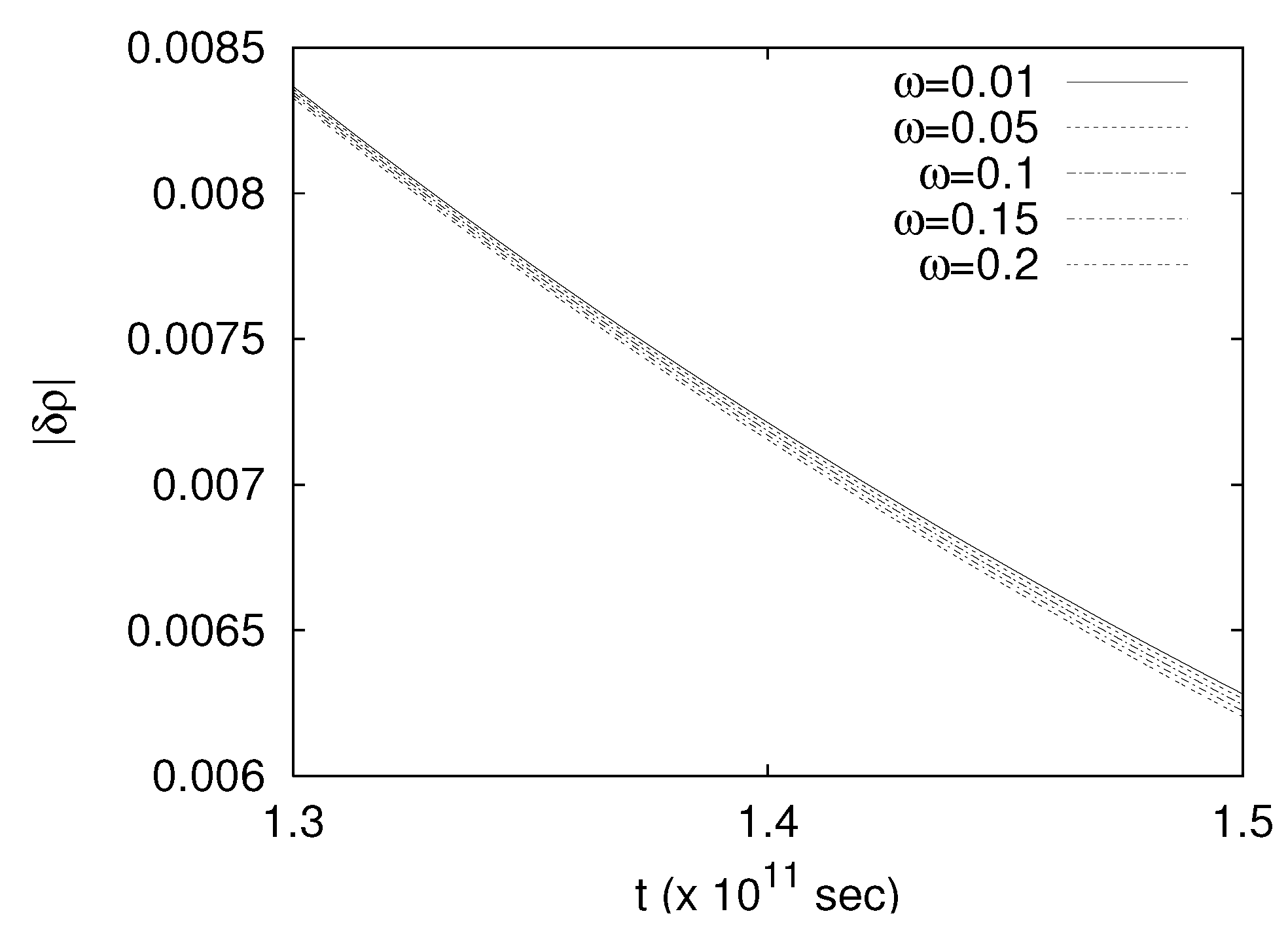The temporal evolution of the GW component $h_{x0}$ (normalized over its initial amplitude) is presented in Figure 1 for $\alpha =1.4$ (the minus sign is nothing but a convention denoting that $|h_{\mu \nu }|$ decreases). In fact, the evolution of $h_{x0}$ is independent of $\alpha$ as a consequence of the constraint given by Equation (31), something that is verified also by the numerical results.

From Figure 1, we observe that the metric perturbation’s amplitude (equivalently, its energy) decreases at a rate $|h_{x0}|\sim t^{-0.58}$, i.e., much steeper than what the cosmological redshift alone would imply, $|h_{x0}|\sim {\left(A^{2}W\right)}^{-1/3}\sim t^{-0.42}$. This is a very important feature of $|h_{x0}|$, suggesting that, apart from Universe expansion, there is an additional descending factor of the GW amplitude, most probably due to the gravitational energy loss in the interaction between gravitational, EM, and the cosmic fluid degrees of freedom (they constitute a closed system). Notice that the same is also true with regards to the evolution of $h_{x\xi }$ and $h_{xv}$.

A potential energy transfer from gravitational to the EM (and the fluid) degrees of freedom due to the resonant interaction between GWs and MHD waves in curved spacetime is an irreversible process, and not only because of the resistivity of the cosmic fluid involved (in connection, see, e.g., [55,56]). In this case, the subsequent damping of the GW has a significant side effect: the production of entropy. The entropy, S, associated with a GW is a natural extension of the quantum von Neumann entropy into classical, four-dimensional wave systems (see, e.g., [57]), i.e.,

$$S=-{\int }_{t_0}^{t}dt{\int }_V{d}^{3}x\sqrt{-g}{\left|h_{x0}\right|}^2\ln {\left|h_{x0}\right|}^2,$$

(56)

where V is the spatial volume involved and $\sqrt{-g}={\left(\frac{t}{t_0}\right)}^{\mathsf{\ell }+1}$ is the determinant of the metric tensor (1). In our case, the GW’s profile does not have any spatial dependence, i.e., its amplitude depends only on time. Therefore, the associated entropy density, $𝒮=S/V$, is given by

$$𝒮=-{\int }_{t_0}^t\sqrt{-g}{\left|h_{x0}\right|}^2\ln {\left|h_{x0}\right|}^{2}dt.$$

(57)

At the initial state $\left(i\right)$, i.e., in the absence of any interaction between GWs and MHD waves, the amplitude of the GW can be written in the form

$$|h_{x0}^{\left(i\right)}|=A\times {\left(\frac{t_0}{t}\right)}^{0.42},$$

(58)

where A is given by Equation (55). On the other hand, at the final state $\left(f\right)$ of the irreversible process under consideration, i.e., in the resonant interaction between GWs and MHD waves, we have

$$|h_{x0}^{\left(f\right)}|=A\times {\left(\frac{t_0}{t}\right)}^{0.58}.$$

(59)

With the aid of Equations (57)–(59), we find that the entropy density variation between the initial and the final state of the GW evolution in its resonant interaction with MHD waves is given by

$$\begin{array}{ccc}\hfill \Delta 𝒮={𝒮}_f-{𝒮}_i& =& \frac{1}{\mathsf{\ell }+0.84}{A}^2{\left(\frac{t}{t_0}\right)}^{\mathsf{\ell }+0.84}\hfill \\ & \times & \left[{\left(\frac{t}{t_0}\right)}^{0.32}\ln \left(\frac{t}{t_0}\right)-\frac{\mathsf{\ell }+0.84}{\mathsf{\ell }+1.16}\ln \left(\frac{A}{t_0}\right)+\left(2\mathsf{\ell }+103.5\right)+𝒪\left(A^{0.75}\right)\right],\hfill \end{array}$$

(60)

where $𝒪\left(A^{0.75}\right)$ denotes terms of the order $A^{0.75}$$\left(\sim {10}^{-8}\right)$. For $\gamma =0.6$$(\mathsf{\ell }=0.25)$ and $1\le \frac{t}{t_0}\le 100$, Equation (60) results in $\Delta 𝒮\simeq 1.3\times {10}^4{A}^2$, which is a definitely positive, although relatively small $\left(\Delta 𝒮\sim {10}^{-18}\right)$, quantity.

On the other hand, the energy, ${\mathcal{E}}_g$, carried by a GW, cannot be defined locally. It can only be quasi-localized under very certain conditions (for more details, see, e.g., [58]). Provided that these conditions are met, the energy carried by a GW is, essentially, proportional to the amplitude square of the GW, i.e., ${\mathcal{E}}_g\sim {\left|h_{x0}\right|}^2$. Hence, an estimate of the gravitational energy lost in the resonant interaction between GWs and MHD waves can be given by comparing the amplitude square of the GW at the aforementioned initial $\left(i\right)$ and final $\left(f\right)$ states of the interaction process. Accordingly,

$$\frac{{\mathcal{E}}_g^{\left(i\right)}}{{\mathcal{E}}_g^{\left(f\right)}}\sim \frac{|h_{x0}^{\left(i\right)}{|}^2}{|h_{x0}^{\left(f\right)}{|}^2}={\left(\frac{t}{t_0}\right)}^{0.32}={100}^{0.32}=4.365.$$

(61)

In view of Equation (61), the GW energy at the beginning of the resonant interaction process is more than four times larger than that at the end of this process. To the best of our knowledge, with the exception of large concentrations of plasma around compact objects, there is no direct conversion of gravitational energy into heat. Therefore, we expect that this energy deficit corresponds to the energy transferred to the EM and the fluid degrees of freedom. However, Equation (61) also reveals a much more interesting feature, namely,

$${\mathcal{E}}_g^{\left(i\right)}\approx 4{\mathcal{E}}_g^{\left(f\right)}\Rightarrow |h_{x0}^{\left(i\right)}|\approx 2|h_{x0}^{\left(f\right)}|.$$

(62)

In other words, if resonant interaction between cosmological GWs (CGWs) and MHD waves has ever taken place in the expansion history of the Universe, then the observed CGW amplitude at the present epoch would be half what would otherwise be expected. Such a result would be an indirect, though quite clear, manifestation that large-scale magnetic fields have indeed played some role in early Universe evolution.

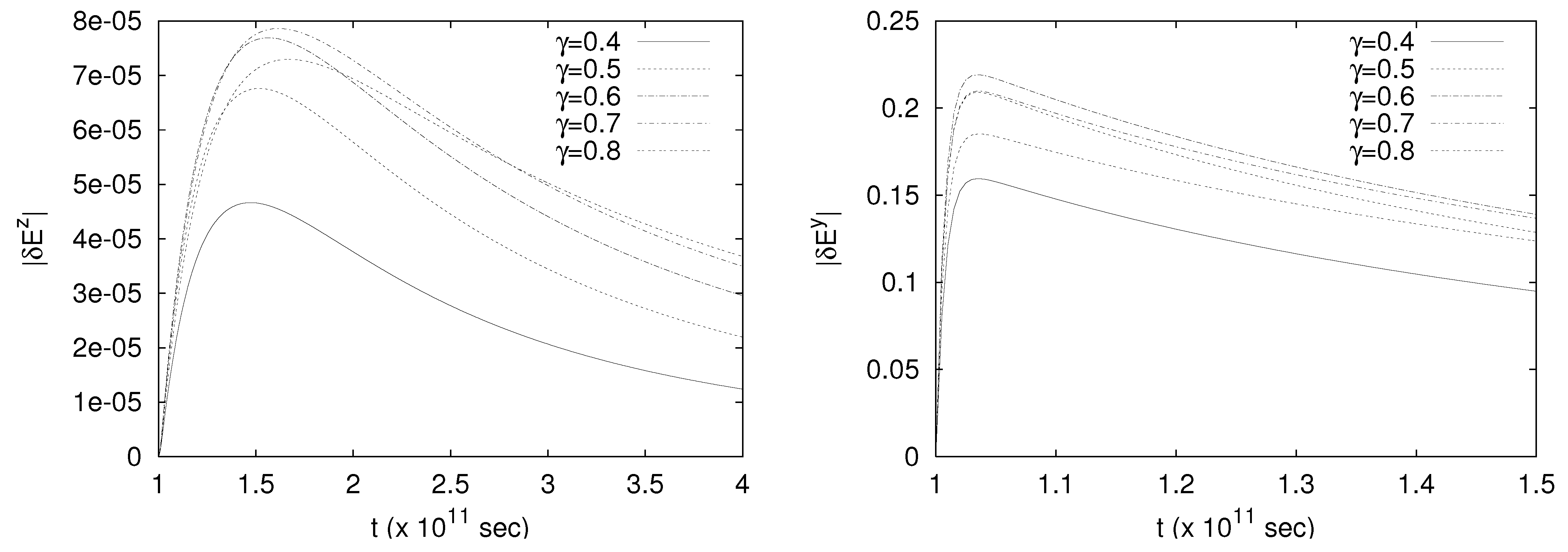
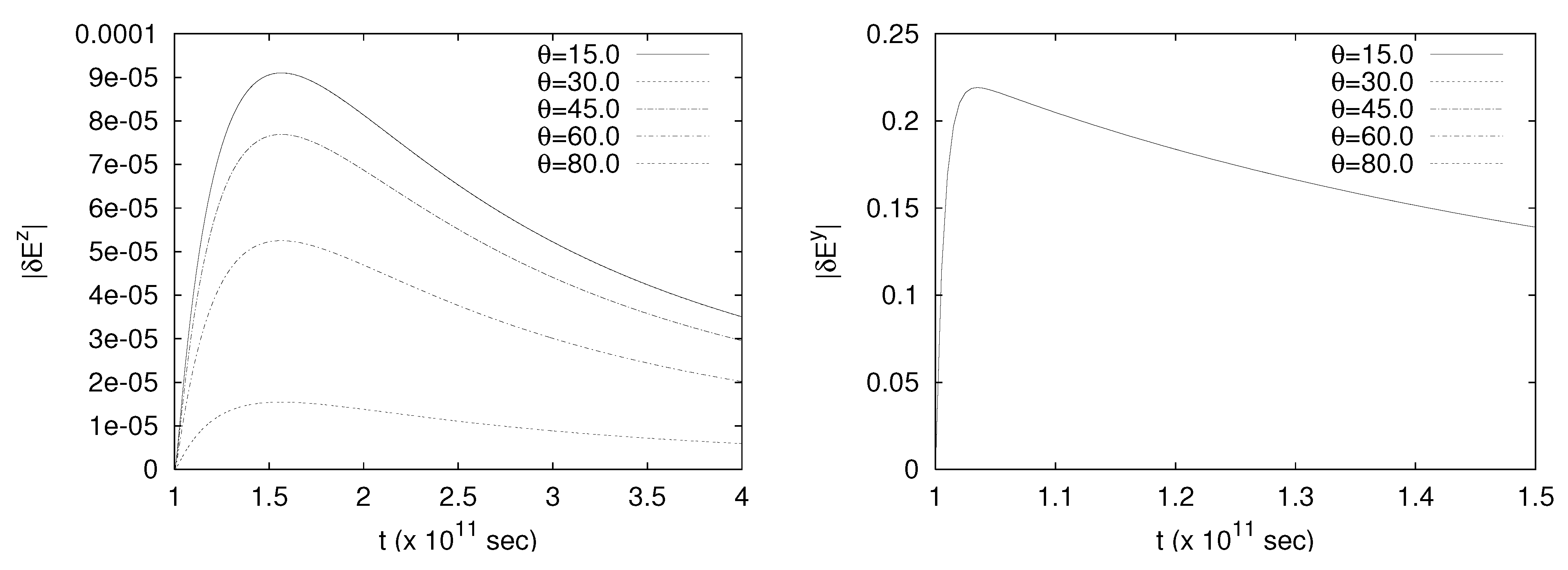
In response to the aforementioned results, we consider the temporal evolution of the electric field perturbations $\delta E^z$ (the Alfvén mode) and $\delta E^y$ (the magnetosonic mode) parametrized by the normalized initial amplitude of the GW, $\alpha$ (Figure 2). We observe that as $\alpha$ increases in absolute value in the range $0.5\le \alpha \le 2.5$, $|\delta E^z|$ almost doubles its maximum value, rising as $|\delta E^z|\sim {\alpha }^{0.44}$, while the magnetosonic component remains unaffected by the variation of $\alpha$, increasing very rapidly to reach an amplitude 2500 times larger than that of $\delta E^z$. On the other hand, the electric field perturbation along the $\widehat{x}-$axis remains null$\left(|\delta E^x|\simeq 0\right)$, i.e., it is not amplified effectively during the whole temporal integration interval, $1\le \frac{t}{t_0}\le 100$.

Now that we have a clear-cut case regarding a GW’s propagation in the magnetized plasma that drives the evolution of Thorne’s model—i.e., it can certainly transfer a part of its energy to the EM field and/or the cosmic fluid degrees of freedom—we may explore the associated response of the various MHD quantities involved. We need to point out that the three linearly independent constraints $c_i=0$$(i=1,2,3)$ arising from Equations (31), (36) and (43) are also monitored throughout numerical integration. During the whole time interval $1\le \frac{t}{t_0}\le 100$, none of them ever exceeds the value ${10}^{-10}$, i.e., they remain sufficiently close to zero. This feature suggests that our model is (indeed) self-consistent, thus making us quite confident of the accuracy of our results despite the complexity of the associated field equations.

4.1. Resistive Instabilities

The first set of parameters to be treated as constants are $\{\gamma =0.6,{\omega }_g=0.1$ Hz, $\theta ={45}^{\circ }\}$. In other words, the angle of propagation with respect to the direction of the magnetic field in Thorne’s spacetime of fixed anisotropy with regard to a transient, non-dispersive, plane GW of $\alpha =1.4$, is also kept fixed at ${45}^{\circ }$. In this case, the evolution of the various MHD modes—basically the electric field perturbations $\delta E^z$ (the Alfvén component) and $\delta E^y$ (the magnetosonic one)—is parametrized only by the conductivity of the plasma fluid. On the basis of its potential temporal dependence during $t_0=t_{eq}\le t\le t_{rec}=100t_0$, a representative set of conductivity values would be $\sigma =\{1.0,5.0,10.0,15.0,20.0\}$. The corresponding results are shown in Figure 3. We observe that the electric field perturbations along the direction of the background magnetic field are, in fact, resistive instabilities, as they are particularly favoured by small values of conductivity (i.e., high values of resistivity). On the contrary, the perturbations along the (normal) $\widehat{y}$-direction (the associated MSWs) increase much more steeply, and they are saturated at high amplitude values (almost 2500 times higher than those of the Alfvén component) for long enough time intervals ($\Delta t\simeq {10}^{12}$ s) in accordance with the increasing conductivity. This is not an unexpected result, since in the large-conductivity (i.e., low resistivity) limit of an ideal plasma, only the magnetosonic component survives (see, e.g., [59]).

In Figure 4, the temporal evolution of the density perturbations in Thorne’s model are presented as a function of conductivity. It becomes evident that high values of conductivity suppress density fluctuations quite rapidly. In other words, low conductivity values—which clearly signal a departure from the ideal plasma case—do favour mass-density instabilities, a result that is in accordance with earlier works [32,59].

4.2. Anisotropic Instabilities

Next, we consider the following set of parameters to be kept constant: $\{\sigma =10.0$ s${}^{-1},{\omega }_g=0.1$ Hz$,\theta ={45}^{\circ }\}$. In this case, the angle of propagation with respect to the direction of the magnetic field in Thorne’s spacetime of variable anisotropy (i.e., magnetic field intensity), as regards a transient, non-dispersive, plane GW, is kept fixed at ${45}^{\circ }$. The non-ideal plasma that drives the evolution of such a spacetime model has a conductivity of $\sigma =10.0$ s${}^{-1}$. Accordingly, the evolution of the various MHD modes—basically the electric field perturbations $\delta E^z$ and $\delta E^y$—is parametrized by the anisotropy measure, $\gamma$, taking values of growing anisotropy, i.e., $\gamma =\{0.4,0.5,0.6,0.7,0.8\}$. The associated results are presented in Figure 5.

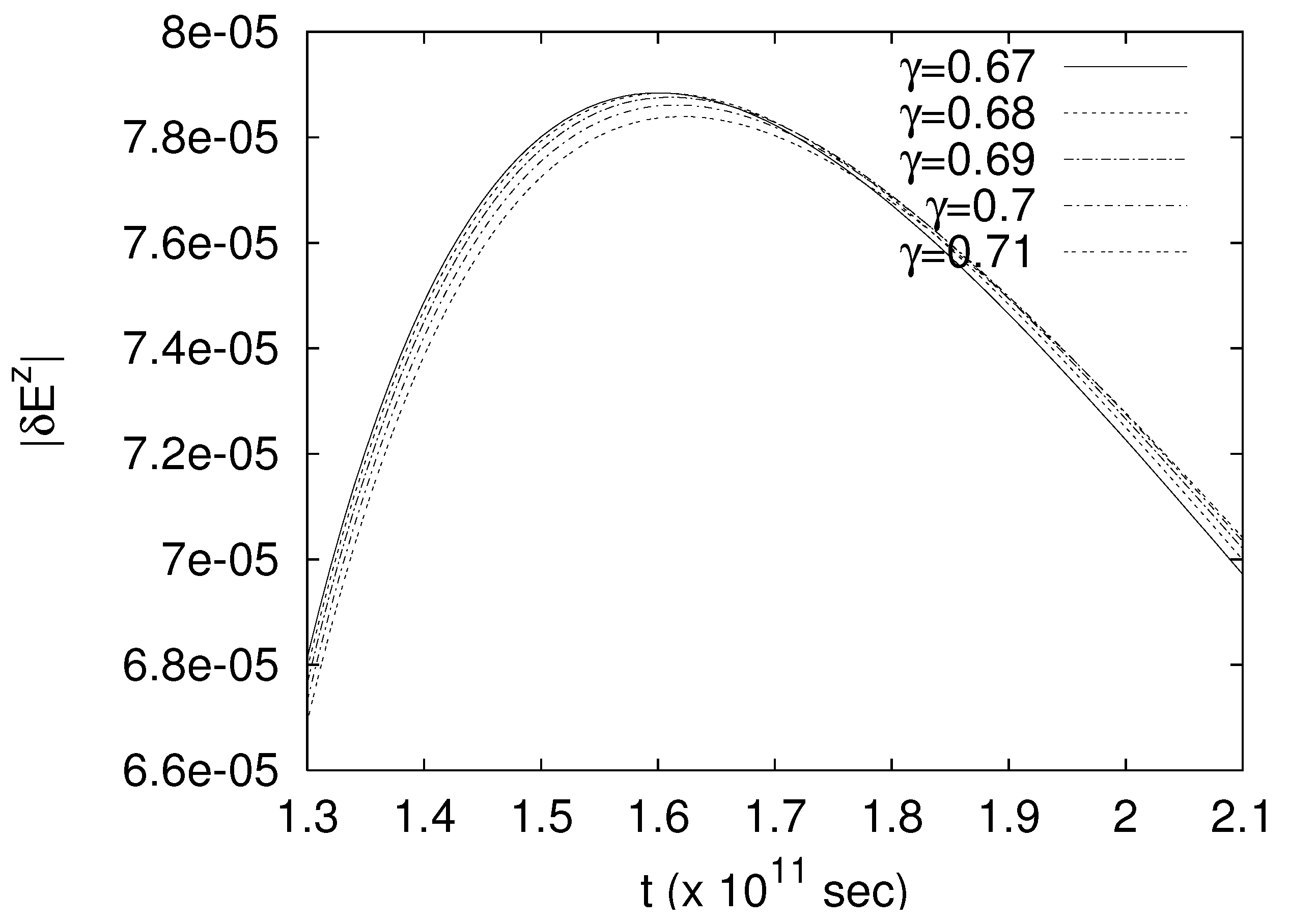
Once again, the magnetosonic component of the electric field perturbation increases more steeply than the corresponding Alfvén one, reaching an amplitude almost 3000 times higher than that of $\delta E^z$. In this case, large values of $\gamma$ correspond to a higher degree of anisotropy of the background spacetime and to a lower expansion rate along the direction of the ambient magnetic field. For $\gamma \ge 0.66$, the magnetic field strength starts to decrease (cf. Equation (3)), and this behaviour is monitored also in the evolution of the electric field (intersecting curves). Indeed, numerics confirm that up to $\gamma \simeq 0.7$, $|\delta E^z|$ rises with the increase in the anisotropy measure, whereas for greater values of $\gamma$, this behaviour is reversed (see, e.g., Figure 6).

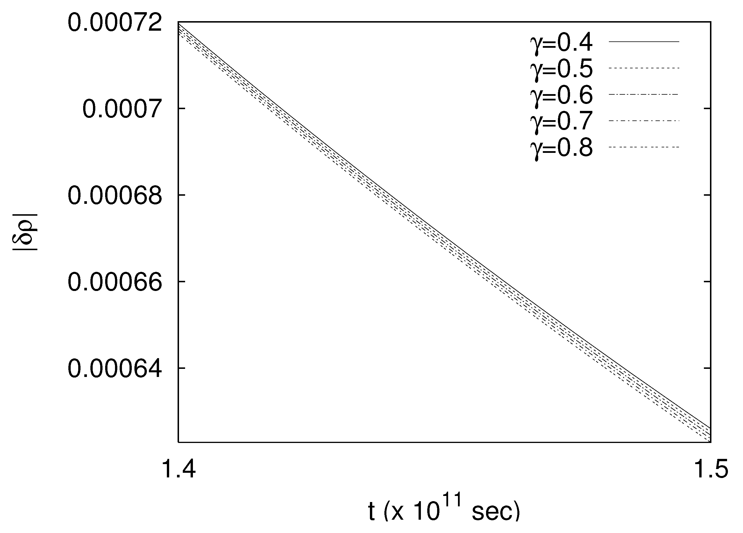
In Figure 7, we illustrate the dependence of the mass-density perturbations on $\gamma$. The corresponding results are displayed over a limited time interval for reasons of best analysis. We observe that the density perturbations decay more rapidly as $\gamma$ grows. Large values of $\gamma$ correspond to a slow expansion rate along the direction of the magnetic field. Therefore, we expect that normal to this direction, condensations that may be formed within the plasma fluid will remain active for longer time intervals, something that could lead to pancake instabilities. It appears that one- and/or two-dimensional formations are actually quite common in magnetized anisotropic cosmological models (see, e.g., [59]).

4.3. Dispersive Instabilities

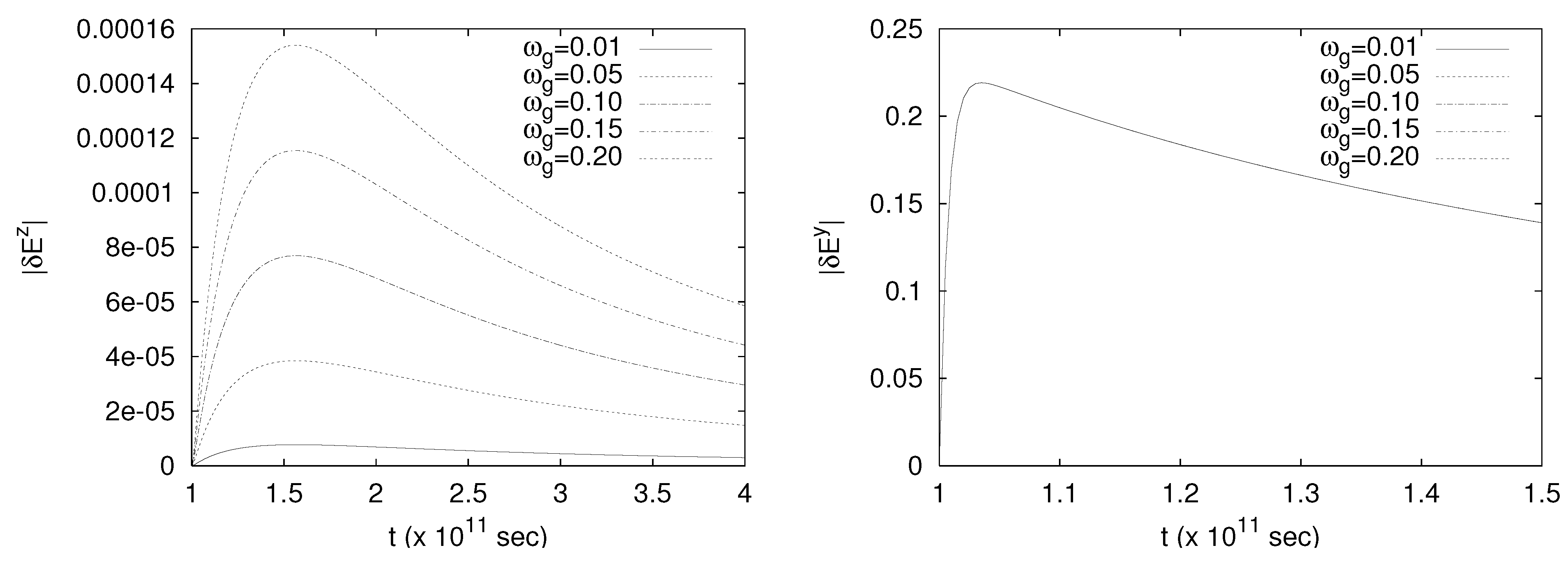
Now, we examine the dependence of the temporal evolution of the electric field perturbations $\delta E^z$ and $\delta E^y$ on the frequency of the GW. To do so, we consider the following set of constants $\{\gamma =0.6,\sigma =10.0{\mathrm{s}}^{-1},\theta ={45}^{\circ }\}$, while ${\omega }_g$ admits the values ${\omega }_g=\{0.01,0.05,0.10,0.15,0.20\}$, measured in $Hz$. This dependence is illustrated in Figure 8. We observe that the electric field perturbation along the direction of the background magnetic field is affected by the variation of the frequency, while that along the $\widehat{y}$-direction remains unaltered. In particular, the first of Figure 8 suggests that high-frequency GWs favour an Alfvén component that grows linearly with ${\omega }_g$, i.e., $|\delta E^z|\sim {\omega }_g$. On the other hand, the independence of $|\delta E^y|$ on ${\omega }_g$ is rather surprising, since in the isotropic model, one would have an ${\omega }_g^2$-dependence (see, e.g., [15]). Instead, here, $|\delta E^y|$ rises very rapidly to reach values 5000 times higher than the Alfvén component and remains almost saturated for a long time interval. This is typical behaviour of the anisotropic magnetosonic instability that we saw earlier (cf. Figure 5 for $\gamma =0.6$). It appears that, regarding MSW propagation in the magnetized plasma under consideration, the spacetime anisotropy prevails over any frequency modulation of the GW.

Furthermore, we observe that a decreasing ${\omega }_g$ (i.e., the long GW wavelength regime) also favours condensations that can be formed within the plasma fluid to remain active for longer time intervals (Figure 9).

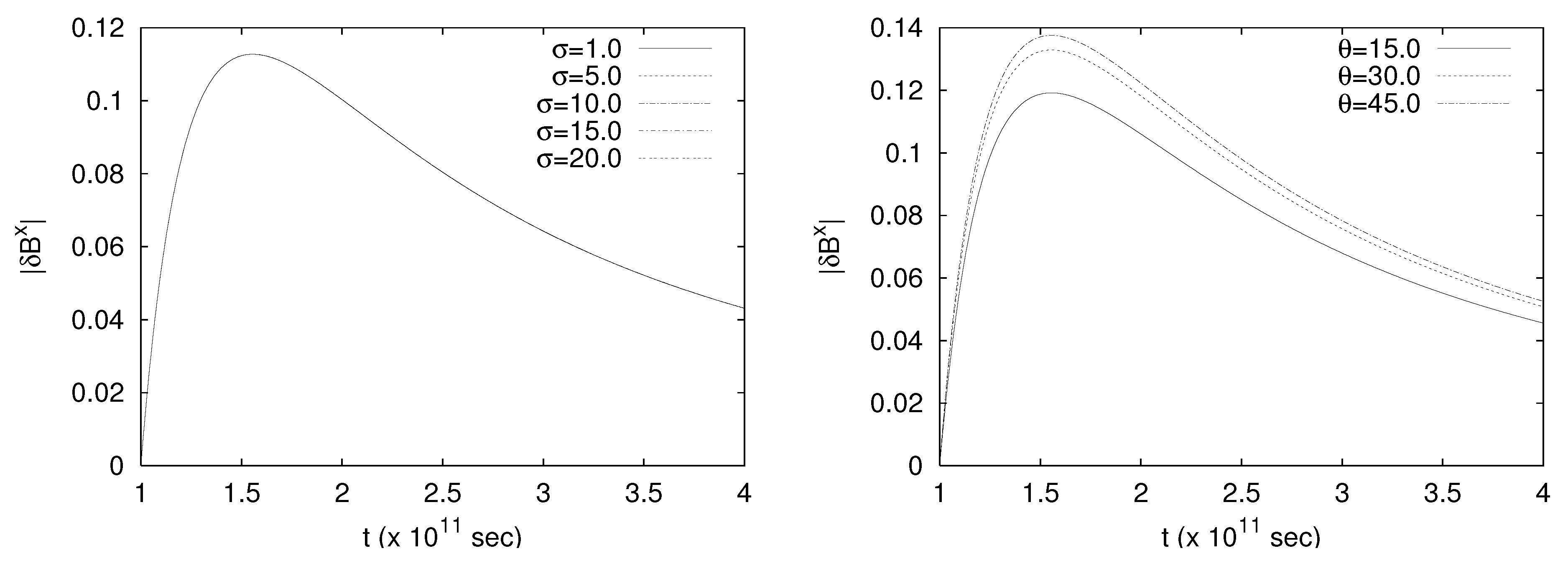
4.4. Resonant Instabilities

To conclude our analysis on the electric field perturbations, we now consider their evolution with respect to the angle of the GW propagation with respect to the direction of the ambient magnetic field of Thorne’s model, i.e., $\theta =\{{15}^{\circ },{30}^{\circ },{45}^{\circ },{60}^{\circ },{80}^{\circ }\}$ (see Figure 10, wherein the following set of parameters are treated as constants: $\{\gamma =0.6,\sigma =10.0$ s${}^{-1},\omega =0.1$ Hz}). In this case, in addition to the magnetosonic component $\delta E^y$, which is always present as a result of the anisotropic instability (independent of $\theta$), as we approach normal propagation ($\theta \to 0^{\circ }$), the Alfvén component $\left(\delta E^z\right)$ is also excited significantly. The reason is that when the wave vector becomes vertical to the direction of the magnetic field, $\delta E^z$ also corresponds to a magnetosonic mode of the system under study.

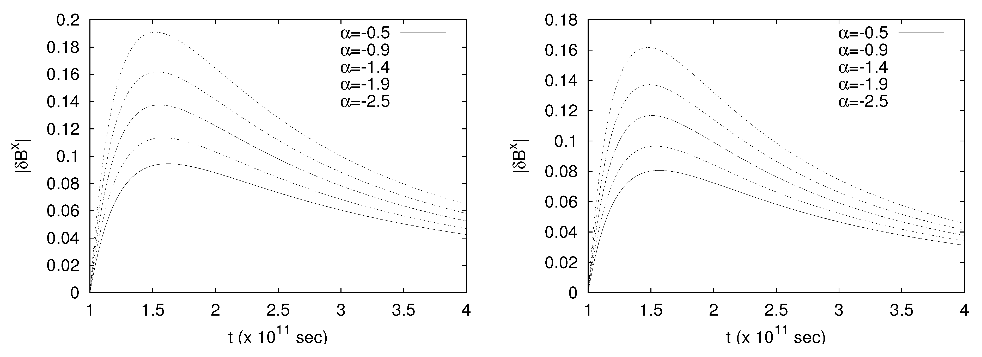
4.5. Magnetic Field Perturbations

Finally, in Figure 11 and Figure 12, we depict the temporal evolution of the magnetic field perturbations parametrized by the normalized initial amplitude of the GW, $\alpha$, the conductivity of the plasma fluid, $\sigma$, and the angle of propagation of the metric perturbation, $\theta$. The numerical results indicate that in this case, only the $\widehat{x}$-component of the magnetic field perturbations (the associated MSW) is excited significantly, probably due to the anisotropic instability that is always present (in connection, see, e.g., [59]). Nevertheless, $\delta B^x$ exhibits also some other, very interesting features. In particular, as $\alpha$ increases in absolute value in the range $0.5\le \alpha \le 2.5$, $|\delta B^x|$ almost doubles its maximum value, rising as $|\delta B^x|\sim {\alpha }^{0.44}$. This is exactly the same behaviour as in the case of the Alfvén electric field perturbation (see Figure 2). It appears that the magnetic field MSWs do get triggered by the GW, while the corresponding electric-field components are driven mainly by the background anisotropy. The opposite behaviour is excited by the associated Alfvén components. Finally, the magnetosonic component $\delta B^x$ appears to be independent of $\sigma$ but not of the angle of propagation, $\theta$, with respect to which it grows as $|\delta B^x|\sim {\theta }^{0.22}$, i.e., it becomes even more prominent on the approach to the parallel propagation case (cf. Figure 12).

5. Discussion and Conclusions

Using the resistive MHD equations in curved spacetime, we investigated numerically the temporal evolution of the electric and magnetic field perturbations, along with the associated mass-density ones, that can be triggered by the oblique propagation of a plane-polarized GW in a class of anisotropic cosmological models with an ambient magnetic field along the $\widehat{z}$-axis, namely, in Thorne’s cosmological model. This model could be a viable extension to the Standard Model of the Early Universe in the presence of a large-scale magnetic field since such a field can affect the local spacetime structure; accordingly, an anisotropic background must be taken into account to guarantee the proper treatment of curved spacetime.

Technically speaking, the GWs affect the evolution of MHD waves in curved spacetime through the general-relativistic Euler equations of motion (18) and the associated Maxwell field Equation (19). The so-assumed gravito–electromagnetic interaction is an irreversible process, mostly due to the backreaction of the EM fields and the fluid on the curved spacetime background through the Einstein field Equations (14)–(16). In this article, by admitting a perfect fluid source, we have actually neglected potential distortions of the curved spacetime background due to energy flows. In general, one could use a non-ideal gas, where the heat conduction, shear, and viscosity of the fluid source should also be taken into account when solving the Einstein field equations. In fact, it would be particularly interesting to examine what would be the exact nature of the aforementioned gravito–electromagnetic interaction in a realistic (i.e., non-ideal) fluid. This will be the scope of future work.

In this article, we are mainly interested in the resonant interaction between GWs and MHD waves, i.e., when the value of the MHD circular frequency is close to the corresponding GW quantity. As we have found, in this case, energy transfer from the gravitational to the EM degrees of freedom does take place, resulting in the excitation of the latter and in the damping of the GW. The various MHD modes excited increase quite rapidly at early times after $t_0$ (where the main resonance $\omega \simeq {\omega }_g$ takes place) to reach a maximum value, while afterwards, they decay at a much lower rate. In some cases, the perturbations (basically, the magnetosonic modes) are saturated at high amplitude values for long enough time intervals, driven by the inherent background anisotropy. In particular, we have identified the following major points:

When a plane-polarized GW propagates in a conductive plasma fluid obliquely to the direction of the ambient magnetic field that drives the evolution of Thorne’s model, its amplitude (equivalently, its energy) decreases at a rate much higher than what the cosmological redshift alone would imply (Figure 1). This result suggests that, apart from Universe expansion, there is an additional descending factor of the GW amplitude, most probably due to the gravitational energy lost in the interaction between gravitational, EM, and the cosmic fluid degrees of freedom, since all of them constitute a closed system. In this context, the GW damping results also in the production of an extra amount of entropy. Indeed, in the resonant interaction between GWs and MHD waves in Thorne’s model, the entropy density variation, $\Delta 𝒮$, between the initial state (when there is no interaction at all) and the corresponding final one (i.e., at the end of the gravito–electromagnetic interaction process) is directly proportional to the amplitude square of the GW involved, which is a definitely positive, although quite small, quantity.

Certainly, the energy carried by a GW cannot be defined locally. However, an estimate of the gravitational energy that is lost in the resonant interaction between GWs and MHD waves can be given by comparing the amplitude square of the GW at the aforementioned initial and final states of the interaction process. Accordingly, we have found that the GW energy at the beginning of the resonant interaction process was more than four times larger than that at the end of this process (cf. Equation (61)). To the best of our knowledge, there is no direct conversion of gravitational energy into heat. Therefore, we expect that this energy deficit corresponds to the energy transferred to the EM and the fluid degrees of freedom. This result, however, might have a much more intriguing consequence, that is, if a resonant interaction between cosmological GWs (CGWs) and MHD waves has ever taken place in the history of Universe expansion, then the observed CGW amplitude at the present epoch would be half what is expected (cf. Equation (62)). Verification of this result by observations would be an indirect, though quite clear, manifestation that large-scale magnetic fields have indeed played some role in the early Universe’s evolution.

In view of the aforementioned results, the temporal evolution of the electric field perturbations $\delta E^z$ (the Alfvén mode) and $\delta E^y$ (the magnetosonic mode) has been examined, parametrized by the normalized initial amplitude of the GW, $\alpha$ (Figure 2). We have found that, as $\alpha$ increases in the range $0.5\le \alpha \le 2.5$, the Alfvén mode $|\delta E^z|$ rises as $|\delta E^z|\sim {\alpha }^{0.44}$. Regarding the associated magnetosonic one, $\delta E^y$, it appears to remain unaffected by the variation of $\alpha$ and increases rapidly after $t_0$, probably because it is trapped in the second resonance, $\omega \simeq 1.005{\omega }_g$. Its amplitude reaches values 2500 times higher than those of $\delta E^z$, where it saturates for a relatively long time interval, probably due to the inherent spacetime anisotropy (anisotropic instability).

On the other hand, regarding the magnetic field perturbations, numerics indicate that only the $\widehat{x}$-component (the associated MSW) is excited significantly, probably due to the anisotropic instability that is always present. The amplitude of $\delta B^x$ also rises with the increasing $\alpha$ as $|\delta B^x|\sim {\alpha }^{0.44}$, i.e., at exactly the same rate as $|\delta E^z|$. It appears that the magnetic field MSWs do get triggered by the GW, while the corresponding electric field components are driven mainly by the background anisotropy. Accordingly, we cannot help but wonder whether the ever-present magnetic field in the Universe has been partly achieved at the expense of gravitational radiation. Clearly, this could be the scope of future work. Notice also that the magnetosonic component $\delta B^x$ appears to be independent of $\sigma$ but not of the angle of propagation, $\theta$, with respect to which its amplitude grows as $|\delta B^x|\sim {\theta }^{0.22}$, i.e., it becomes even more prominent on the approach to the parallel propagation case (cf. Figure 12).

As for the response of the electric components to the variation of the cosmological parameters involved, such as the conductivity of the plasma fluid (resistive instabilities), the anisotropy measure of the curved spacetime (anisotropic instabilities), the frequency modulation of the GW (dispersive instabilities), and the variation of the associated angle of propagation with respect to the direction of the magnetic field (resonant instabilities), it can be summarized as follows:

Resistive instabilities: Numerical results suggest that the electric field perturbations along the direction of the background magnetic field are particularly favoured by low conductivity (i.e., high resistivity) values (Figure 3). Regarding the perturbations along the (normal) $\widehat{y}$-direction (the associated MSWs), they increase much more steeply and they are saturated at high amplitude values (almost 2500 times higher than those of the Alfvén component) for much longer time intervals ($\Delta t\simeq {10}^{12}$ s) in accordance with growing conductivity. This is not an unexpected result, since in the large $\sigma$ limit (i.e., approaching the ideal plasma case), only the magnetosonic component survives.

Anisotropic instabilities: When anisotropy grows, the magnetosonic component of the electric field perturbation increases steeply and its amplitude reaches values almost 3000 times higher than those of $\delta E^z$. Large values of the associated measure,$\gamma$, correspond to a lower expansion rate along the direction of the ambient magnetic field. For $\gamma \ge 0.66$, the magnetic field strength also starts to decrease (cf. Equation (3)), and this behaviour is monitored also in the evolution of the electric components (cf. Figure 5). Indeed, the numerical results confirm that up to $\gamma \simeq 0.7$, $|\delta E^z|$ rises with the increase in the anisotropy measure, whereas for greater values of $\gamma$, this behaviour is reversed (cf. Figure 6).

Dispersive instabilities: Regarding the dependence of the electric modes on the frequency of the GW, we have found that high-frequency GWs favour the Alfvén component, which grows linearly with ${\omega }_g$. On the contrary, $\delta E^y$ appears to be independent of ${\omega }_g$, rising steeply to reach values 5000 times higher than those of $\delta E^z$ and remaining saturated for a relatively long time interval. This is typical behaviour of anisotropic magnetosonic instability; hence, regarding the propagation of MSWs in the magnetized plasma under consideration, the spacetime anisotropy prevails over any frequency modulation of the GW.

Resonant instabilities: In this case, in addition to the magnetosonic component $\delta E^y$, which is always present (independent $\theta$), as we approach normal propagation ($\theta \to 0^{\circ }$), the Alfvén component $\delta E^z$ is also excited significantly. The reason is that when the wave vector becomes vertical to the direction of the magnetic field, $\delta E^z$ also corresponds to a magnetosonic mode of the system.

Rest mass-density fluctuations: Numerics indicate that the rest mass-density perturbations decay more rapidly as $\gamma$ grows. Large values of $\gamma$ correspond to a low expansion rate along the direction of the magnetic field; hence, we expect that normal to this direction, condensations that may be formed within the plasma fluid will remain active for longer time intervals, something that could lead to a two-dimensional (pancake) instability. On the other hand, large conductivity values suppress mass-density fluctuations quite rapidly. In other words, low conductivity, which signals a departure from the ideal plasma case, may favour mass-density instabilities (resistive Jeans instabilities). Finally, long-wavelength GWs (i.e., low ${\omega }_g$ values) also favour density fluctuations to remain active for long time intervals.

To the best of our knowledge, this is the first time that all these kinds of instabilities have been collectively examined in Thorne’s model, a viable extension to the Standard Model of Universe expansion. Clearly, a comprehensive study regarding the excitation of MHD modes (and their subsequent temporal evolution) by GWs in curved spacetime is not only far from being exhausted but, in fact, looks very promising. Therefore, the interaction between gravitational and MHD waves in curved spacetime should be further explored and scrutinized in the search for the most accurate profile of many astrophysical and/or cosmological processes.