
Fitting Power Spectrum of Scalar Perturbations for Primordial Black Hole Production during Inflation


1
Interdisciplinary Research Laboratory, Tomsk State University, Tomsk 634050, Russia
2
Department of Physics, Tokyo Metropolitan University, Hachioji-shi 192-0397, Japan
3
Kavli Institute for the Physics and Mathematics of the Universe (WPI), The University of Tokyo Institutes for Advanced Study, Kashiwa 277-8583, Japan
*
Author to whom correspondence should be addressed.
Astronomy 2023, 2(1), 47-57; https://doi.org/10.3390/astronomy2010005
Submission received: 20 February 2023
/
Revised: 14 March 2023
/
Accepted: 16 March 2023
/
Published: 22 March 2023
Abstract
:A simple phenomenological fit for the power spectrum of scalar (curvature) perturbations during inflation is proposed to analytically describe slow roll of inflaton and formation of primordial black holes (PBH) in the early universe, in the framework of single-field models. The fit is given by a sum of the power spectrum of slow-roll inflation, needed for a viable description of the cosmic microwave background (CMB) radiation in agreement with Planck/BICEP/Keck measurements, and the log-normal (Gaussian) fit for the power spectrum enhancement (peak) needed for efficient PBH production, in the leading (model-independent) approximation. The T-type -attractor models are used to get the simple CMB power spectrum depending upon the e-folds as the running variable. The location and height of the peak are chosen to yield the PBH masses in the asteroid-size window allowed for the whole (current) dark matter. We find the restrictions on the peak width.
1. Introduction
The inflationary paradigm was initially proposed as a possible solution to the internal problems of the standard (Einstein-Friedmann) cosmology such as the horizon problem, the flatness problem and the problem of initial conditions [1,2]. It was later recognized that inflation in the early universe may be a solution to the structure formation problem also [3]. A major recognition of the inflationary paradigm came with its success in explaining the inhomogeneity and anisotropy of the cosmic microwave background (CMB) radiation [4].
The underlying physics of inflation is still unknown but there is no shortage of theoretical models of inflation. The simplest single-field models of chaotic inflation are based on the quintessence (scalar-tensor gravity) or the modified -gravity theories. More recently, the quintessence models were further generalized by adding a near-inflection point to the inflaton potential below the inflationary scale, leading to a peak in the power spectrum of scalar perturbations that later collapse to primordial black holes (PBH) [5,6,7,8].1 PBH are also considered as a good (non-particle) candidate for the present dark matter [13,14].
Usually, one begins with a particular inflationary model having a specific scalar potential, and then one numerically derives the power spectrum by using the Mukhanov-Sasaki equation [15,16]. In this paper, we begin with analytic modeling of the power spectrum of scalar (curvature) perturbations for possible PBH production in agreement with CMB measurements. We choose the simplest fit as a sum of the CMB power spectrum in the slow-roll approximation and the log-normal shape of the peak. This allows us to get analytic smooth sewing of both spectra with the minimal number of parameters and a possibility to analytically explore the whole parameter space, which is often difficult in a numerical approach. As regards the CMB power spectrum, we describe it with the help of the T-type -attractor models of inflation [17,18,19] in order to get the simplest form of the spectrum during slow roll. As a result, we find new restrictions on the parameters of PBH production.
Our paper is organized as follows. In Section 2 we briefly review the T-type -attractor models of inflation, which are used as the viable models for CMB in the next Sections. The power spectrum of scalar perturbations during inflation in the slow-roll approximation (relevant to CMB) is derived in Section 3. Section 4 is devoted to our fit of the power spectrum of scalar perturbations for both CMB and PBH production, and the related spectrum of induced gravitational waves (GW). Our conclusion is Section 5.
2. Single-Field Models of Slow-Roll Inflation for CMB
As the simple models of large-single-field inflation, described by the standard quintessence action
we choose the T-type -attractors [17,18] with the canonical inflaton potential
where the constant specifies the scale of inflation, and the is the free parameter of the order one.
This model is a viable model of large-field slow-roll inflation with a nearly flat potential, whose inflationary solution is an attractor describing chaotic inflation, being very close to the Starobinsky model [20] in the case of . The CMB tilt of scalar perturbations, predicted by the T-model is given by the simple formula [21]
in terms of e-folds as the running variable describing time evolution, as the function of scale k [22]. The CMB tensor-to-scalar ratio r is approximately given by [17,18]
providing the comfortable theoretical prediction against future measurements of r. Indeed, the current CMB measurements by Planck/BICEP/Keck collaborations [23,24,25] give
while they are in good agreement with Equations (3) and (4) with the best fit close to .
The generalization of the simplest T-model potential (2) to the form [17,18]
with a monotonically increasing (during slow roll) function , , can be used for engineering a near-inflection point in the potential, leading to a peak (enhancement) in the power spectrum of scalar perturbations, needed for PBH formation [26,27].2
In the generalized T-models (6) slow-roll inflation occurs for large positive values of the inflation field with an approximate scalar potential of the E-type [30] as
where we have introduced the parameters and . The constant in front of the second term in Equation (7) can be chosen at will by a constant shift of the inflaton field , so that the potential (7) can be simplified to
which implies Equations (3) and (4).
The -attractors with do not have a simple description on the dual -gravity side, see e.g., Ref. [31] for details of the correspondence. The Starobinsky function on the modified gravity side arises in the case of and , where is the inflaton (scalaron) mass. In general, the exact dual gravity function associated with any inflaton potential V in the model (1) is only known in the parametric (implicit) form, see Equations (2.7) and (2.8) in Ref. [31], as
When , or in the slow-roll approximation with the potential (2), we find that the F-function can be approximated in the form
with the function
where is the standard slow-roll parameter
and in terms of the Hubble function H and the potential V.
The particular examples of the generalized T-models, suitable for inflation and PBH production, can be obtained by expanding the -function in Taylor series and tuning the expansion coefficients [26,30].
The slow-roll evolution of inflaton with e-folds N as the running (time) variable is described by the (non-linear) equation of motion, obtained from the standard (Klein-Gordon) equation minimally coupled to gravity in the (spatially flat) universe, when the acceleration term is ignored,
This equation has an exact solution in the case of the T-model potential (2), with
where the (implicit) integration constant is associated with constant shifts of the field . The solution implies
and gives a very simple potential of the T-model in the slow-roll approximation,
The Hubble function is also simply related to the potential is the slow-roll approximation via the Friedmann equation
The relations between the potential , the running tensor-to-scalar ratio and the slow-roll parameter in the slow-roll approximation are very simple too,
leading to a bit more precise formula than Equation (4).
The very simple form (17) of the T-potential in the slow-roll approximation is one of the reasons why we choose the T-models as our baseline models in this paper.
3. Power Spectrum of Scalar Perturbations in Slow-Roll Approximation
Primordial scalar perturbations () and primordial tensor perturbations (primordial gravitational waves g) are defined by a perturbed Friedmann-Lemaitre-Robertson-Walker (FLRW) metric,
where
in terms of the local basis obeying the relations , and .
The primordial spectrum of scalar (density) perturbations is defined by the 2-point correlator of scalar perturbations,
The CMB power spectrum can be described by the Harrison-Zeldovich fit
near the pivot scale , or in the slow-roll (SR) approximation by
The power spectrum is simply related to the potential in the slow-roll approximation via the standard relation, see e.g., Refs. [5,29],
It also implies
In the case of the potential (17), we find very simple equations,
and
where the last equation reproduces Equation (3).
The observed CMB window into inflation does not allow us to reconstruct the full inflaton scalar potential from the power spectrum beyond the slow-roll region. The well-known reconstruction formula, proposed by Hodges and Blumentahl [22] in the form
requires knowing the full power spectrum at different scales and the limits of integration. Moreover, the reconstruction procedure should be based on getting exact solutions to the Mukhanov-Sasaki equation instead of the slow-roll solution in Equation (27), see e.g., Ref. [32] for some examples. It is not our purpose in this paper to reconstruct the inflaton potential beyond its qualitative features. Nevertheless, it may be possible for the CMB region under some additional assumptions, e.g., when assuming a very low value of the tensor-to-scalar ratio r, which implies a small correction to the constant defining the inflationary scale, i.e., the inflaton potential in the form with . Then Equation (29) is simplified to
while the integration constants merely rescale and shift N. Equation (14) also gets simplified to
Then a partial reconstruction of the scalar potential becomes possible from the CMB power spectrum of scalar perturbations without knowing the power spectrum of tensor perturbations, which is also true for the -attractors when the parameter is small enough, , with
as in Equation (8). This is yet another reason for us to take the T-models of -attractors as our baseline models of inflation and generalize their power spectrum of scalar perturbations by adding a peak at higher values of k.
4. Log-Normal Fit for a Peak and GW Spectrum
The log-normal fit is the simplest (Gaussian) description of a peak in the power spectrum, see e.g., Ref. [33]. A power-law ansatz for the peak was considered in Ref. [34]. In this paper we propose another ansatz for the power spectrum, combining the CMB spectrum in the slow-roll approximation with the log-normal fit for the enhancement (peak) of the power spectrum needed for PBH formation at a lower scale,
where is a position of the peak, is the width of the peak and A is the normalization of the peak amplitude, , needed for efficient PBH production (about higher than the CMB amplitude). The normalization factor is given by Equation (27),
see also Equation (24). When , and , we get . The power spectrum (33) can be rewritten, using the e-foldings variable N via the relation
to the simple form
We choose .
We choose or to get within the current observational window for PBH as the whole dark matter [9,10,11], i.e., between g and g. For example, when , we get g. The profile of the power spectrum in given on Figure 1 for some values of .
It follows from Equation (38) versus Equation (3) that the tilt gets the exponentially small corrections (back reaction) from the peak. To quantitatively evaluate an impact of the back reaction, we introduce the dimensionless parameters for the relative scales,
characterizing the separation between the CMB pivot scale and the left end of the peak, and the separation between the end of inflation and the right end of the peak, respectively. Since the CMB pivot scale and the PBH scales have to be separated, it implies or . The exponential corrections in Equation (38) are negligible when . On the other hand, the right end of the peak must be within inflation, so that . We expect to be close to the end of inflation.3
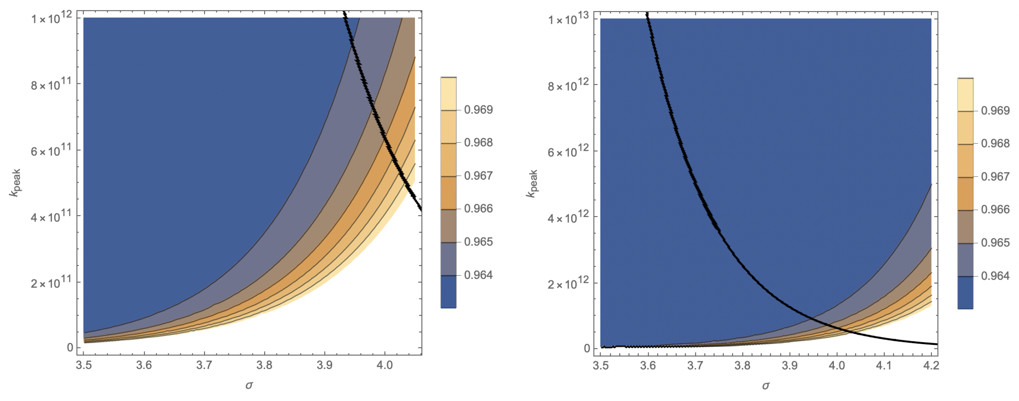
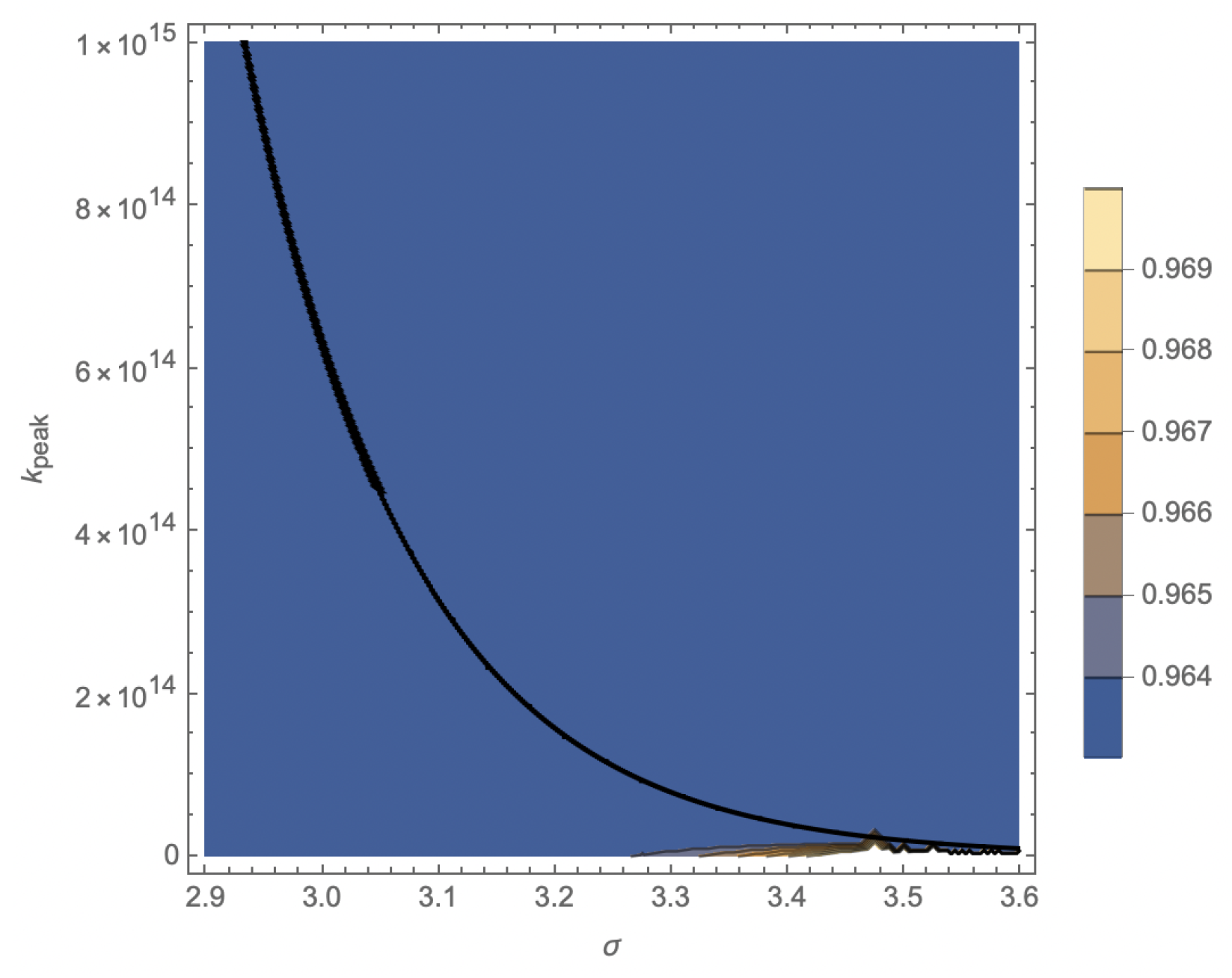
We illustrate those considerations by our numerical calculations with the results displayed on Figure 2 and Figure 3 for various values of and against the observed values of the tilt in Equation (5). The black curves in the (-plane correspond to the condition . The area above the black curve and the white area are forbidden.
For example, when and (or ), we get from Equation (28), whereas we get after taking into account the exponential terms in Equation (38) with the parameters and .
Our analysis allows us to restrict (from above) the possible peak width values at fixed and duration of inflation (or ). We summarize those restrictions in Table 1.4
The spectrum of the induced GW can be derived by using the standard formula obtained in the second order with respect to perturbations [36],
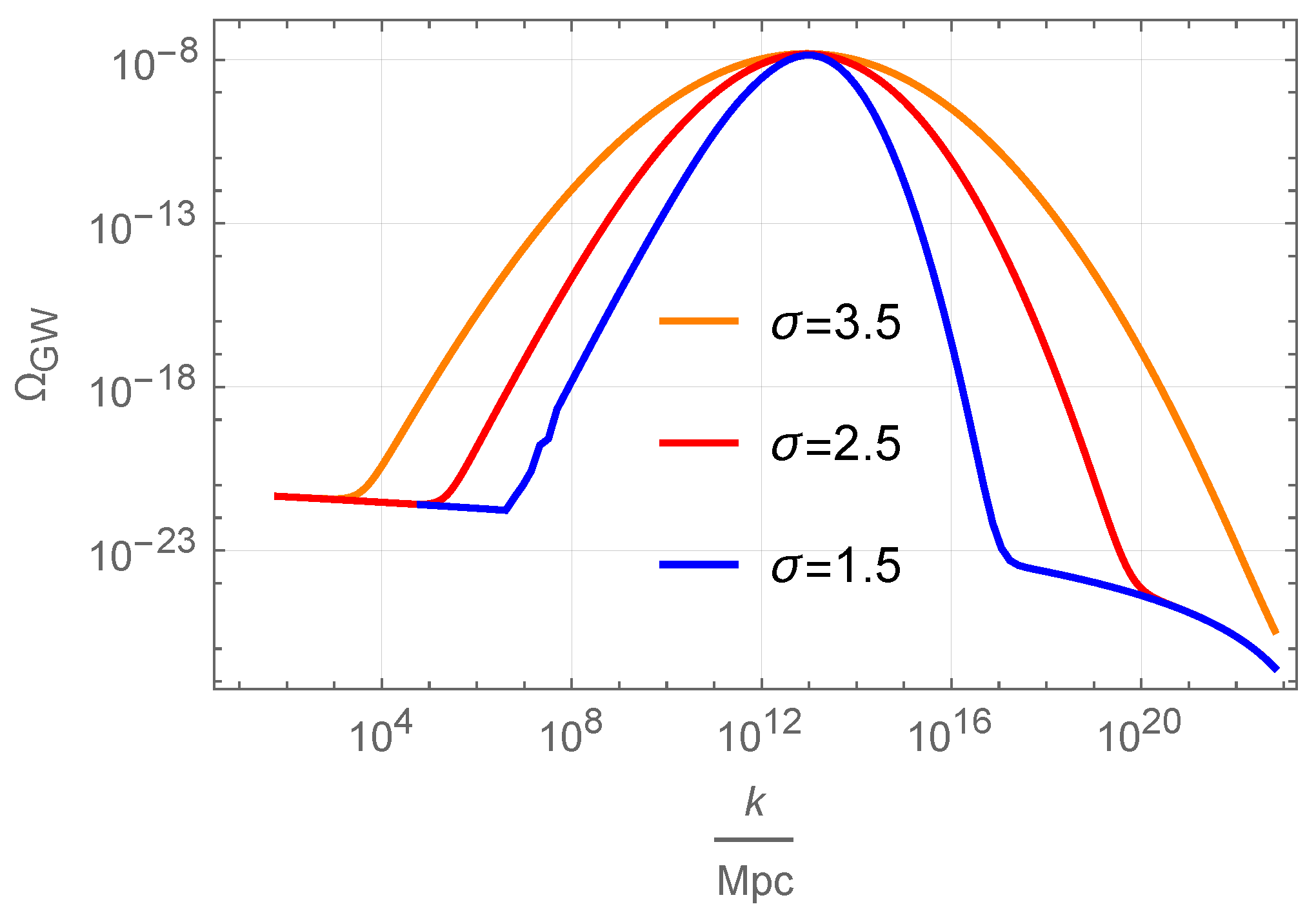
where . Our numerical results for a wide peak with are displayed on Figure 4.
The peak in the GW-spectrum associated with a wide () peak in the power spectrum can be analytically approximated as
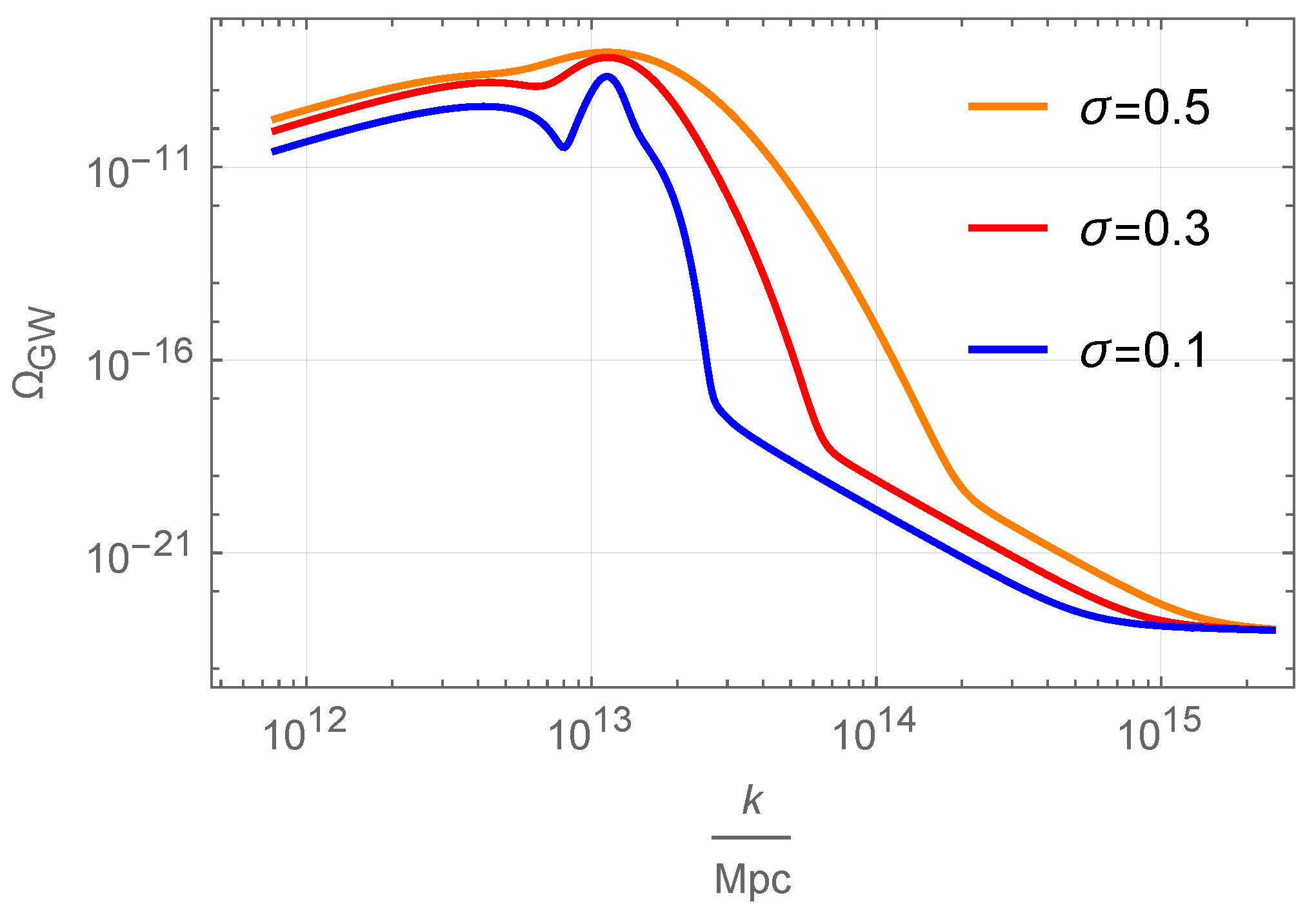
For comparison, in Figure 5 we give our numerical results for the induced GW spectrum with selected values of a sharp peak in the power spectrum. Then the GW spectrum is not given by a sum of contributions from the peak and the slow-roll, while the simple relation to the power spectrum in Equation (41) is also not valid. Instead, the cross terms in Equation (40) become significant and the shape of the GW spectrum changes, see Figure 5. This phenomenon was also observed in Ref. [37].
5. Conclusions
Our investigation in this paper is based on the ansatz (33) for the power spectrum of scalar (curvature) perturbations during inflation. The ansatz is given by a sum of the CMB power spectrum in the slow-roll approximation and the log-normal fit for the power spectrum enhancement (peak) needed for efficient PBH production. The ansatz (33) is very simple, while we use the slow-roll approximation and the T-type -attractor models of inflation in order to justify the first term in Equation (33). The second term in Equation (33) requires the scalar potential in those models to be generalized, e.g., via engineering a near-inflection point and an ultra-slow-roll phase during inflation, see e.g., Refs. [5,6,12,26,27,28,29,30,38,39] for explicit examples. We are aware that the slow-roll approximation is violated during the ultra-slow-roll phase needed for a peak generation, and do not expect that Equation (33) is suitable for a full reconstruction of the inflaton scalar potential. Instead, we take the power spectrum (33) for granted and study its consequences, both analytically and numerically, in the context of CMB and PBH as DM.
Author Contributions
All authors contributed equally to this investigation. All authors have read and agreed to the published version of the manuscript.
Funding
This work was partially supported by Tomsk State University under the development program Priority-2030. SVK was also supported by Tokyo Metropolitan University, the Japanese Society for Promotion of Science under the grant No. 22K03624, and the World Premier International Research Center Initiative, MEXT, Japan.
Institutional Review Board Statement
Not applicable.
Informed Consent Statement
Not applicable.
Data Availability Statement
No new data was created.
Acknowledgments
One of the authors (SVK) is grateful to Shyam Balaji, Guillem Domenech, Noriaki Kitazawa, Laura Iacconi, Misao Sasaki and Alexei Starobinsky for discussions and correspondence.
Conflicts of Interest
The authors declare no conflict of interest.
| 1 | |
| 2 | |
| 3 | Particle production is also more efficient toward the end of inflation [35]. |
| 4 | When , the PBH masses are lower than the Hawking evaporation limit of for black holes. |
References
- Guth, A.H. The Inflationary Universe: A Possible Solution to the Horizon and Flatness Problems. Phys. Rev. D 1981, 23, 347–356. [Google Scholar] [CrossRef] [Green Version]
- Linde, A.D. A New Inflationary Universe Scenario: A Possible Solution of the Horizon, Flatness, Homogeneity, Isotropy and Primordial Monopole Problems. Phys. Lett. B 1982, 108, 389–393. [Google Scholar] [CrossRef]
- Liddle, A.R.; Lyth, D.H. Cosmological Inflation and Large Scale Structure; Cambridge University Press: Cambrdige, UK, 2000. [Google Scholar]
- Mukhanov, V. Physical Foundations of Cosmology; Cambridge University Press: Oxford, UK, 2005. [Google Scholar] [CrossRef] [Green Version]
- Garcia-Bellido, J.; Ruiz Morales, E. Primordial black holes from single field models of inflation. Phys. Dark Univ. 2017, 18, 47–54. [Google Scholar] [CrossRef] [Green Version]
- Germani, C.; Prokopec, T. On primordial black holes from an inflection point. Phys. Dark Univ. 2017, 18, 6–10. [Google Scholar] [CrossRef] [Green Version]
- Germani, C.; Musco, I. Abundance of Primordial Black Holes Depends on the Shape of the Inflationary Power Spectrum. Phys. Rev. Lett. 2019, 122, 141302. [Google Scholar] [CrossRef] [Green Version]
- Bhaumik, N.; Jain, R.K. Primordial black holes dark matter from inflection point models of inflation and the effects of reheating. JCAP 2020, 1, 37. [Google Scholar] [CrossRef] [Green Version]
- Sasaki, M.; Suyama, T.; Tanaka, T.; Yokoyama, S. Primordial black holes—Perspectives in gravitational wave astronomy. Class. Quant. Grav. 2018, 35, 63001. [Google Scholar] [CrossRef] [Green Version]
- Carr, B.; Kohri, K.; Sendouda, Y.; Yokoyama, J. Constraints on primordial black holes. Rept. Prog. Phys. 2021, 84, 116902. [Google Scholar] [CrossRef]
- Escrivà, A.; Kuhnel, F.; Tada, Y. Primordial Black Holes. arXiv 2022, arXiv:2211.05767. [Google Scholar]
- Karam, A.; Koivunen, N.; Tomberg, E.; Vaskonen, V.; Veermäe, H. Anatomy of single-field inflationary models for primordial black holes. arXiv 2022, arXiv:2205.13540. [Google Scholar] [CrossRef]
- Barrow, J.D.; Copeland, E.J.; Liddle, A.R. The Cosmology of black hole relics. Phys. Rev. D 1992, 46, 645–657. [Google Scholar] [CrossRef] [PubMed]
- Garcia-Bellido, J.; Linde, A.D.; Wands, D. Density perturbations and black hole formation in hybrid inflation. Phys. Rev. D 1996, 54, 6040–6058. [Google Scholar] [CrossRef] [PubMed] [Green Version]
- Mukhanov, V.F. Gravitational Instability of the Universe Filled with a Scalar Field. JETP Lett. 1985, 41, 493–496. [Google Scholar]
- Sasaki, M. Large Scale Quantum Fluctuations in the Inflationary Universe. Prog. Theor. Phys. 1986, 76, 1036. [Google Scholar] [CrossRef] [Green Version]
- Kallosh, R.; Linde, A. Universality Class in Conformal Inflation. JCAP 2013, 7, 2. [Google Scholar] [CrossRef] [Green Version]
- Galante, M.; Kallosh, R.; Linde, A.; Roest, D. Unity of Cosmological Inflation Attractors. Phys. Rev. Lett. 2015, 114, 141302. [Google Scholar] [CrossRef] [Green Version]
- Ellis, J.; Garcia, M.A.G.; Nanopoulos, D.V.; Olive, K.A.; Verner, S. BICEP/Keck constraints on attractor models of inflation and reheating. Phys. Rev. D 2022, 105, 43504. [Google Scholar] [CrossRef]
- Starobinsky, A.A. A new type of isotropic cosmological models without singularity. Phys. Lett. B 1980, 91, 99–102. [Google Scholar] [CrossRef]
- Mukhanov, V.F.; Chibisov, G.V. Quantum Fluctuations and a Nonsingular Universe. JETP Lett. 1981, 33, 532–535. [Google Scholar]
- Hodges, H.M.; Blumenthal, G.R. Arbitrariness of inflationary fluctuation spectra. Phys. Rev. D 1990, 42, 3329–3333. [Google Scholar] [CrossRef]
- Akrami, Y.; Arroja, F.; Ashdown, M.; Aumont, J.; Baccigalupi, C.; Ballardini, M.; Savelainen, M. Planck 2018 results. X. Constraints on inflation. Astron. Astrophys. 2020, 641, A10. [Google Scholar] [CrossRef] [Green Version]
- Ade, P.A.R.; Ahmed, Z.; Amiri, M.; Barkats, D.; Thakur, R.B.; Bischoff, C.A.; Bicep/Keck Collaboration. Improved Constraints on Primordial Gravitational Waves using Planck, WMAP, and BICEP/Keck Observations through the 2018 Observing Season. Phys. Rev. Lett. 2021, 127, 151301. [Google Scholar] [CrossRef]
- Tristram, M.; Banday, A.J.; Górski, K.M.; Keskitalo, R.; Lawrence, C.R.; Andersen, K.J.; Wehus, I.K. Improved limits on the tensor-to-scalar ratio using BICEP and Planck data. Phys. Rev. D 2022, 105, 83524. [Google Scholar] [CrossRef]
- Iacconi, L.; Assadullahi, H.; Fasiello, M.; Wands, D. Revisiting small-scale fluctuations in α-attractor models of inflation. JCAP 2022, 6, 7. [Google Scholar] [CrossRef]
- Braglia, M.; Linde, A.; Kallosh, R.; Finelli, F. Hybrid α-attractors, primordial black holes and gravitational wave backgrounds. arXiv 2022, arXiv:2211.14262. [Google Scholar]
- Frolovsky, D.; Ketov, S.V.; Saburov, S. Formation of primordial black holes after Starobinsky inflation. Mod. Phys. Lett. A 2022, 37, 2250135. [Google Scholar] [CrossRef]
- Frolovsky, D.; Ketov, S.V.; Saburov, S. E-models of inflation and primordial black holes. Front. Phys. 2022, 10, 1005333. [Google Scholar] [CrossRef]
- Dalianis, I.; Kehagias, A.; Tringas, G. Primordial black holes from α-attractors. JCAP 2019, 1, 37. [Google Scholar] [CrossRef] [Green Version]
- Ivanov, V.R.; Ketov, S.V.; Pozdeeva, E.O.; Vernov, S.Y. Analytic extensions of Starobinsky model of inflation. JCAP 2022, 3, 58. [Google Scholar] [CrossRef]
- Dudas, E.; Kitazawa, N.; Patil, S.P.; Sagnotti, A. CMB Imprints of a Pre-Inflationary Climbing Phase. JCAP 2012, 5, 12. [Google Scholar] [CrossRef]
- Pi, S.; Sasaki, M. Gravitational Waves Induced by Scalar Perturbations with a Lognormal Peak. JCAP 2020, 9, 37. [Google Scholar] [CrossRef]
- Hertzberg, M.P.; Yamada, M. Primordial Black Holes from Polynomial Potentials in Single Field Inflation. Phys. Rev. D 2018, 97, 83509. [Google Scholar] [CrossRef] [Green Version]
- Addazi, A.; Ketov, S.V.; Khlopov, M.Y. Gravitino and Polonyi production in supergravity. Eur. Phys. J. C. 2018, 78, 642. [Google Scholar] [CrossRef]
- Domènech, G. Scalar Induced Gravitational Waves Review. Universe 2021, 7, 398. [Google Scholar] [CrossRef]
- Balaji, S.; Domenech, G.; Silk, J. Induced gravitational waves from slow-roll inflation after an enhancing phase. JCAP 2022, 9, 16. [Google Scholar] [CrossRef]
- Ragavendra, H.V.; Saha, P.; Sriramkumar, L.; Silk, J. Primordial black holes and secondary gravitational waves from ultraslow roll and punctuated inflation. Phys. Rev. D 2021, 103, 83510. [Google Scholar] [CrossRef]
- Balaji, S.; Silk, J.; Wu, Y.P. Induced gravitational waves from the cosmic coincidence. JCAP 2022, 6, 8. [Google Scholar] [CrossRef]
Figure 1.
The power spectrum with the parameters , , for .

Figure 2.
The impact of Equation (38) on the parameters of our model for (on the left) and for (on the right) in the -plane. The (excluded) area above the black curve leads to the right end of the peak after the end of inflation. The other parameters are and .
Figure 2.
The impact of Equation (38) on the parameters of our model for (on the left) and for (on the right) in the -plane. The (excluded) area above the black curve leads to the right end of the peak after the end of inflation. The other parameters are and .

Figure 3.
The impact of Equation (38) on the parameters for in the -plane. The (excluded) area above the black curve leads to the right end of the peak after the end of inflation. The other parameters are and .
Figure 3.
The impact of Equation (38) on the parameters for in the -plane. The (excluded) area above the black curve leads to the right end of the peak after the end of inflation. The other parameters are and .

Figure 4.
The induced GW spectrum for selected values of a wide peak in the power spectrum, with the parameters , and .
Figure 4.
The induced GW spectrum for selected values of a wide peak in the power spectrum, with the parameters , and .

Figure 5.
The induced GW spectrum for selected values of a sharp peak in the power spectrum, with the parameters , and .
Figure 5.
The induced GW spectrum for selected values of a sharp peak in the power spectrum, with the parameters , and .


Table 1.
The PBH masses , the scales and the upper bounds on .
| ≤3.89 | ||
| ≤3.73 | ||
| ≤3.56 | ||
| ≤3.40 | ||
| ≤3.23 |
Disclaimer/Publisher’s Note: The statements, opinions and data contained in all publications are solely those of the individual author(s) and contributor(s) and not of MDPI and/or the editor(s). MDPI and/or the editor(s) disclaim responsibility for any injury to people or property resulting from any ideas, methods, instructions or products referred to in the content. |
© 2023 by the authors. Licensee MDPI, Basel, Switzerland. This article is an open access article distributed under the terms and conditions of the Creative Commons Attribution (CC BY) license (https://creativecommons.org/licenses/by/4.0/).
Share and Cite
MDPI and ACS Style
Frolovsky, D.; Ketov, S.V. Fitting Power Spectrum of Scalar Perturbations for Primordial Black Hole Production during Inflation. Astronomy 2023, 2, 47-57. https://doi.org/10.3390/astronomy2010005
AMA Style
Frolovsky D, Ketov SV. Fitting Power Spectrum of Scalar Perturbations for Primordial Black Hole Production during Inflation. Astronomy. 2023; 2(1):47-57. https://doi.org/10.3390/astronomy2010005
Chicago/Turabian StyleFrolovsky, Daniel, and Sergei V. Ketov. 2023. "Fitting Power Spectrum of Scalar Perturbations for Primordial Black Hole Production during Inflation" Astronomy 2, no. 1: 47-57. https://doi.org/10.3390/astronomy2010005