Communication

(No) Eternal Inflation in the Starobinsky Inflation Corrected by Higher Curvature Invariants

Faculty of Physics, University of Warsaw, 00-927 Warszawa, Poland
*
Authors to whom correspondence should be addressed.
Astronomy 2023, 2(1), 15-21; https://doi.org/10.3390/astronomy2010003
Submission received: 18 November 2022 / Revised: 1 February 2023 / Accepted: 10 February 2023 / Published: 22 February 2023

Abstract

:
The swampland criteria in string theory assert the no eternal inflation scenario. This work studied the impact of generic gravitational quantum corrections on eternal inflation. In particular, we find that the Starobinsky model of inflation should receive higher-order corrections stemming from quantum gravity. In this work, we studied the effect of the R 3 / 2 and R 4 corrections on the eternal inflation conditions for the Starobinsky model.

1. Introduction

The swampland conjectures state that not every consistent quantum field theory can be UV completed by string theory [1]; for reviews, see [2,3] and the references therein. In the cosmological context, one of the most-prominent swampland restrictions is the de-Sitter conjecture, which states that there is no stable de-Sitter vacuum1. In mathematical terms, the de-Sitter conjecture states that given potential V ( ϕ ) ,
M P | V | V > c O ( 1 ) ,
has to hold.
On the other hand, the most-popular Early Universe cosmological scenario is inflation, which relies on the quasi-de-Sitter phase. During inflation, an effective scalar field caused the accelerated expansion of the Universe. The inflaton evolution starts at the flat potential region, then the field “rolls” down to a local minimum, where it oscillates, producing the Standard Model particles. On top of the classical evolution, quantum fluctuations induce spatial inhomogeneities that can be in principle observed. The smoking gun of the inflationary scenario would be a detection of the primordial gravitational waves (which, so far, have not been discovered); see the Planck Collaboration’s results [9]. Furthermore, the time evolution of the scalar field is stochastic in nature due to the quantum fluctuations. This local, stochastic behavior can drive the field “upwards” the inflationary potential, leading to pocket Universes. Regions of space that cease to inflate are rapidly dominated and, after a sufficiently long time, become a measure zero set. In particular, for a stochastic evolution to dominate the classical rolling, one requires the effective potential to be sufficiently flat:
| V | V 3 2 < 2 2 π 1 M P 3 , V V < 3 M P 2 .
On the other hand, eternal inflation is potentially problematic since it spoils the predictive power stemming from the inflationary scenario. It creates causally disconnected patches of the Universe where inflation ends at various times, creating different initial conditions. In principle, the other patches are impossible to probe from our own patch. For a summary of the arguments, see [10,11], and for other views, see, e.g., [12]. Furthermore, there is a clear tension between eternal inflation (2) and the swampland de-Sitter Conjecture (1).
Thus, the (no) eternal inflation principle was put forward [13] within string theory. It is then important to study whether other quantum gravity approaches also forbid the eternal inflation scenario. In particular, the above equations provide a simple test of whether the swampland conjectures hold within the postulated theory. In our previous work [14], we verified the applicability of Condition (2) (and further conditions stemming from the no eternal inflation principle) for a handful of asymptotically safe (AS) inflationary models [15,16,17,18]. Effective inflationary potentials derived from AS theories are generally flat at large field values. In turn, eternal inflation occurs, given the field’s initial value is large. This conclusion is compatible with a direct numerical simulation of the Langevin equation and the semi-analytical approach of the swampland conditions.
Here, we extend our analysis by studying the generic quantum corrections to the Starobinsky inflation, which are expected to play a role when approaching the Planck scale. The following sections discuss how the Starobinsky model fits into the eternal inflation picture and consider its extensions.

2. Mechanism of Eternal Inflation

In this section, we briefly introduce the mechanism for eternal inflation. The action of the scalar inflaton is given by
S = d 4 𝘨 1 2 M P 2 R + 1 2 𝘨 μ ν μ ϕ ν ϕ V ( ϕ ) .
The effective potential may be derived from a strictly gravitational action (containing no matter fields) by transforming from the Jordan to the Einstein frame [19]. Assuming a homogeneous distribution of the field ϕ ( t , x ) = ϕ ( t ) , one obtains the following equations of motion:
ϕ ¨ + 3 H ϕ + V ϕ = 0 , H 2 M P 2 = 1 3 1 2 ϕ ˙ 2 + V ( ϕ ) ,
which, in the slow-roll approximation, become [20]
3 H ϕ ˙ + V ϕ 0 , H 2 M P 2 1 3 V ϕ .
Inflation ends once one of the so-called slow-roll parameters becomes of order one:
ϵ M P 2 2 V , ϕ V 2 , η M P 2 V , ϕ ϕ V ,
and enters the oscillatory, reheating phase. The standard treatment of eternal inflation relies on the stochastic inflation approach [21], and for the remainder of this section, we follow [13]. One splits the field into the classical background and short-wavelength quantum field:
ϕ t , x = ϕ c l t , x + δ ϕ t , x .
Since the action is quadratic in the fluctuations, one may approximate the late-time evolution with Langevin equation:
3 H ϕ ˙ + V ϕ = N t ,
where N t is a normally distributed noise term with mean equal to 0 and variance σ = H 3 t 4 π 2 [22]. With this setup, the probability density P [ ϕ , t ] , that at time t, the field has value ϕ governed by the Fokker–Planck equation:
P ˙ [ ϕ , t ] = 1 2 H 3 4 π 2 2 P [ ϕ , t ] ϕ ϕ + 1 3 H i i V ϕ P [ ϕ , t ] ,
where P ˙ [ ϕ , t ] : = t P [ ϕ , t ] . For a constant potential, the Fokker–Planck equation reduces to the heat equation and follows an unbiased Gaussian distribution. The linear potential leads to a Gaussian distribution with μ = ϕ c l a s ( t ) , where ϕ c l a s is the value of the field in the classical potential. Furthermore, most of the inflationary potentials are flat at ϕ and, hence, can be Taylor expanded around infinity, which considerably simplifies the analysis2. Then, for large field values, the solutions will be approximately exponential, and the probability, that the inflation is still ongoing, is
Pr [ ϕ > ϕ e n d , t ] = ϕ c d ϕ P [ ϕ , t ] C ( t ) exp ( Γ t ) ,
where function C ( t ) is a polynomial and parameter Γ is the decay rate. It is then clear that, at the large-time limit, the inflation should stop, since
Pr [ ϕ > ϕ e n d , t ] 0 as t + .
However, during inflation, the scale factor grows exponentially, and the size of the Universe depends on time according to:
U t = U 0 e 3 H t ,
where U 0 is the initial volume of the pre-inflationary Universe. One then interprets the probability P r [ ϕ > ϕ e n d , t ] as a fraction of the volume U i n f t still inflating, that is
U i n f t = U 0 e 3 H t P r [ ϕ > ϕ e n d , t ] ,
then, in order for the Universe to inflate eternally, the positive exponential factor 3 H in Equation (13) and the exponential factor Γ must satisfy:
3 H > Γ .
One may show that this stochastic bound is equivalent to (2), assuming that we approximate the effective potential with, a respectively, a linear and quadratic hilltop. Numerical investigations based on the Langevin equation give the same conditions for eternal inflation as the analytical criteria (2) [14].

3. Eternal Inflation in Starobinsky-Like Models

3.1. Starobinsky Inflation
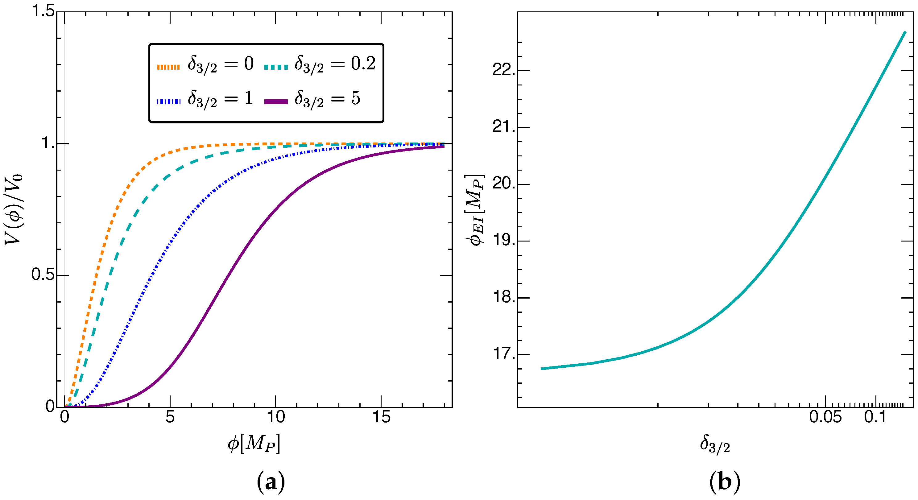
The Starobinsky model of inflation was proposed as an alternative to General Relativity, which could describe the non-singular beginning of the Universe [23]. It is one of the most-promising theories of inflation when it comes to the CMB measurements of the spectral tilt n s and predicts the low value of the tensor-to-scalar ratio r. In the context of quantum gravity, the action of Starobinsky inflation should be understood as the lowest-order expansion of the full gravitational effective action:
S = M P 2 2 d x 4 𝘨 R + 1 6 m 2 R 2 + O ( R 3 ) ,
where m is the inflaton mass. The effective potential obtained in the Einstein frame is
V ( ϕ ) = 3 4 M P 2 m 2 1 y 2 ,
where
y = exp 2 3 ϕ M P
and the CMB data fix m = 10 5 M P for the constraints on inflationary models; see [9]. The 60 e-folds are realized for the initial value of the field, given as ϕ 0 = 5.5   M P . Applying the eternal Conditions (13) results in the ϕ E I = 16   M P bound for eternal inflation. The super-Planckian values of the field suggest that strictly classical theory (15) may not be valid in the regime of quantum gravity. This leads us to considerations of modified Starobinsky models with higher curvature corrections.
Recently, several models extending Starobinsky inflation have been proposed [24]. These models derive the inflationary potential from the Lagrangian terms of higher-order in the Ricci scalar. In this section, we briefly introduce the R + R 2 + R 3 / 2 and R + R 2 + R 4 models and their effective inflationary potentials. The quartic model3 does not lead to the multiverse scenario, while being in good agreement with the CMB data.

3.2. Eternal Inflation for R 3 / 2 Correction

The R 3 / 2 term appears in the chiral modified super-gravity and the asymptotic safety fixed point effective action [16] with Λ = 0 . The action is given by
S = M P 2 2 d x 4 𝘨 R + 1 6 m 2 R 2 Starobinsky model + δ 3 / 2 m R 3 / 2 .
Parameter δ 3 / 2 describes the strength of the coupling. The effective potential is given by
V = 4 V 0 σ ˜ ( 3 δ 3 / 2 σ ˜ + σ ˜ ) ( 6 + 9 + δ 3 / 2 σ ˜ + 2 σ ˜ ) 2 ,
where
σ ˜ = 3 ( 1 y ) y + 9 δ 3 / 2 8 y 9 δ 3 / 2 y 3 y ( 27 δ 3 / 2 2 y 16 y + 16 )
and y is given by (17). After matching to the amplitude of scalar perturbation, the coupling δ 3 / 2 is the only free parameter in the theory. The left panel in Figure 1a shows the shape of the potential. In the limit δ 3 / 2 0 , the original Starobinsky model is recovered. Increasing δ 3 / 2 shifts the slope towards greater field values. This is important from the eternal inflation point of view, since the quantum fluctuations dominate at the potential plateau. A minimal initial value of the field, above which inflation becomes eternal, is ϕ E I = 16.7   M P l , for δ 3 / 2 = 0 . Figure 1b shows how this value changes with the coupling. This result can be directly computed with (1). However, as is usually the case, the first condition is the most-restrictive one. The conditions for higher derivatives do not give new information. It was found in [24] that the CMB data allow for values even of order δ 3 / 2 = 100 . We can see that eternal inflation “kicks in” at extremely large values of ϕ ; for δ 3 / 2 = 0.15 , it is around ϕ E I = 30   M P l . It is still possible, however, for a different set of initial conditions (in a neighboring pocket Universe) to allow for eternal inflation creating a multiverse.

3.3. Eternal Inflation for the R 4 Correction

We now move our attention to a R 4 theory also described in detail by [24]. The action of the Starobinsky model corrected by a quartic term is
S = M P 2 2 d x 4 𝘨 = M P 2 2 R + 1 6 m 2 R 2 + δ 4 48 m 6 R 4 ,
where δ 4 is a dimensionless parameter. For δ 4 > 0 , the mass spectrum is positive, thus avoiding the ghost degrees of freedom. The effective potential is
V = V 0 σ ˜ 2 ( 8 + 3 σ ˜ δ 4 ) ( 12 + 4 σ ˜ + δ 4 σ ˜ 3 ) 2 ,
where
σ ˜ = Z 3 δ 4 4 Z and Z = δ 4 2 / 3 162 ( y 1 1 ) + 6 3 243 ( y 1 1 ) 2 + 16 δ 4 1 1 3 .
Parameter y is given by (17). The shape of the above potential is depicted in Figure 2a. The slow-roll inflation here is qualitatively different from the δ 4 = 0 case. Inflation starts around the maximum of the potential and may roll down both to the right and to the left of the top. Slow-roll conditions are always violated at the bottom of each branch. This means that classical inflation lasts a finite time. Quantum fluctuations, however, could, in principle, “hold” the inflaton around the peak. The condition on the first Derivative (2) is depicted in Figure 2b. Both conditions are satisfied in the range between ( 1 , 11 )   M P . In the presence of multiple minima, tunneling between vacua can occur due to Gaussian fluctuations, modeled by the Langevin Equation (8).
In particular, for a model discussed in [17], the Conditions (2) implied that there is no eternal inflation. However, at the same time, an explicit simulation revealed that there is a possibility of eternal inflation.
Interestingly, for the model with the R 4 corrections, field rolling to either of the minima leads to the inflationary period’s end. Hence, inflation has a well-defined end in both branches, and the quantum tunneling phenomena described above cannot drive eternal inflation. One may consider initial conditions at different points in the very Early Universe to be scattered around Figure 2a including the large field values. The region of the Universe with the initial value ϕ 0 around ϕ m a x will grow exponentially fast and dominate regions with ϕ 0 ϕ m a x , where the slow-roll does not occur. This means inflation will not become eternal regardless of the initial conditions and the value of the only free parameter in theory δ 4 > 0 . To the authors’ best knowledge, this is the only known inflation model agreeing with the CMB data, which generally does not produce eternal inflation, at large field values.

4. Conclusions

Eternal inflation is a conceptual issue of the inflationary birth of the Universe [11]. Our analysis revealed no obstruction for the eternal inflation scenario in the effective quantum-gravity-safe models. On the other hand, quantum corrections lift the scale of eternal inflation. In particular, for the R 4 correction, there is no eternal inflation regime at large field values.

Author Contributions

Conceptualization, J.C. and J.H.K.; software, J.C. and J.H.K.; calculations, J.C.; writing—original draft preparation, J.C. and J.H.K.; writing—review and editing, J.H.K.; visualization, J.H.K. All authors have read and agreed to the published version of the manuscript.

Funding

J.H.K. was supported by the Polish National Science Centre Grant 2018/29/N/ST2/01743.

Institutional Review Board Statement

Not applicable.

Informed Consent Statement

Not applicable.

Data Availability Statement

Not applicable.

Conflicts of Interest

The authors declare no conflict of interest.

References

  1. Vafa, C. The String Landscape and the Swampland. arXiv 2005, arXiv:hep-th/0509212. [Google Scholar]
  2. Brennan, T.D.; Carta, F.; Vafa, C. The String Landscape, the Swampland, and the Missing Corner. arXiv 2017, arXiv:1711.00864. [Google Scholar]
  3. Palti, E. The Swampland: Introduction and Review. Fortsch. Phys. 2019, 67, 1900037. [Google Scholar] [CrossRef] [Green Version]
  4. Meissner, K.A.; Veneziano, G. Symmetries of cosmological superstring vacua. Phys. Lett. B 1991, 267, 33–36. [Google Scholar] [CrossRef] [Green Version]
  5. Meissner, K.A.; Veneziano, G. Manifestly O(d,d) invariant approach to space-time dependent string vacua. Mod. Phys. Lett. A 1991, 6, 3397–3404. [Google Scholar] [CrossRef] [Green Version]
  6. Meissner, K.A. Symmetries of higher order string gravity actions. Phys. Lett. B 1997, 392, 298–304. [Google Scholar] [CrossRef] [Green Version]
  7. Hohm, O.; Zwiebach, B. Non-perturbative de Sitter vacua via α corrections. Int. J. Mod. Phys. D 2019, 28, 1943002. [Google Scholar] [CrossRef] [Green Version]
  8. Hohm, O.; Zwiebach, B. Duality invariant cosmology to all orders in α’. Phys. Rev. D 2019, 100, 126011. [Google Scholar] [CrossRef] [Green Version]
  9. Akrami, Y.; Arroja, F.; Ashdown, M.; Aumont, J.; Baccigalupi, C.; Ballardini, M.; Banday, A.J.; Barreiro, R.B.; Bartolo, N.; Basak, S.; et al. Planck 2018 results. X. Constraints on inflation. Astron. Astrophys. 2020, 641, A10. [Google Scholar] [CrossRef] [Green Version]
  10. Ijjas, A.; Steinhardt, P.J.; Loeb, A. Inflationary paradigm in trouble after Planck 2013. Phys. Lett. B 2013, 723, 261–266. [Google Scholar] [CrossRef]
  11. Ijjas, A.; Steinhardt, P.J.; Loeb, A. Inflationary schism. Phys. Lett. B 2014, 736, 142–146. [Google Scholar] [CrossRef] [Green Version]
  12. Guth, A.H.; Kaiser, D.I.; Nomura, Y. Inflationary paradigm after Planck 2013. Phys. Lett. B 2014, 733, 112–119. [Google Scholar] [CrossRef] [Green Version]
  13. Rudelius, T. Conditions for (no) eternal inflation. J. Cosmol. Astropart. Phys. 2019, 2019, 009. [Google Scholar] [CrossRef] [Green Version]
  14. Chojnacki, J.; Krajecka, J.; Kwapisz, J.; Slowik, O.; Strag, A. Is asymptotically safe inflation eternal? J. Cosmol. Astropart. Phys. 2021, 2021, 076. [Google Scholar] [CrossRef]
  15. Bonanno, A.; Platania, A. Asymptotically safe inflation from quadratic gravity. Phys. Lett. B 2015, 750, 638–642. [Google Scholar] [CrossRef]
  16. Platania, A. From renormalization group flows to cosmology. Front. Phys. 2020, 8, 188. [Google Scholar] [CrossRef]
  17. Nielsen, N.G.; Sannino, F.; Svendsen, O. Inflation from Asymptotically Safe Theories. Phys. Rev. D 2015, 91, 103521. [Google Scholar] [CrossRef] [Green Version]
  18. Svendsen, O.; Bazrafshan Moghaddam, H.; Brandenberger, R. Preheating in an Asymptotically Safe Quantum Field Theory. Phys. Rev. D 2016, 94, 083527. [Google Scholar] [CrossRef] [Green Version]
  19. Kaiser, D.I. Conformal Transformations with Multiple Scalar Fields. Phys. Rev. D 2010, 81, 084044. [Google Scholar] [CrossRef] [Green Version]
  20. Liddle, A.R.; Parsons, P.; Barrow, J.D. Formalizing the slow-roll approximation in inflation. Phys. Rev. D 1994, 50, 7222–7232. [Google Scholar] [CrossRef]
  21. Linde, A.D. Hard art of the Universe creation (stochastic approach to tunneling and baby Universe formation). Nucl. Phys. B 1992, 372, 421–442. [Google Scholar] [CrossRef] [Green Version]
  22. Linde, A. Stochastic approach to tunneling and baby Universe formation. Nucl. Phys. B 1992, 372, 421–442. [Google Scholar] [CrossRef] [Green Version]
  23. Starobinsky, A.A. A New Type of Isotropic Cosmological Models without Singularity. Phys. Lett. B 1980, 91, 99–102. [Google Scholar] [CrossRef]
  24. Ivanov, V.R.; Ketov, S.V.; Pozdeeva, E.O.; Vernov, S.Y. Analytic extensions of Starobinsky model of inflation. arXiv 2021, arXiv:2111.09058. [Google Scholar] [CrossRef]
1
For the discussion on the non-perturbative de-Sitter vacua based on the O ( d , d ) construction, see [4,5,6], see [7,8].
2
We thank Astrid Eichhorn for pointing this out.
3
The model with the correction R 3 leads to a similar shape of the potential. Its agreement with the CMB, however, is restricted to a much narrower range of the coupling values.
Figure 1. (a) The R 3 / 2 model effective potential for various δ . (b) Plot of the minimal initial value ϕ E I , above which the inflation becomes eternal as a function of the coupling value.
Astronomy 02 00003 g001
Figure 2. (a) The R 4 model effective potential. The yellow line corresponds to the δ 4 = 0 limit of Starobinsky inflation. Non-zero δ 4 introduces a right branch of the inflationary potential (blue curve). In such cases, the slow roll may be realized in both directions. (b) Plot of the first of the Conditions (1). Eternal inflation does not dominate large field values. It can only occur around the top of the hill. However, this effect is unstable: quantum fluctuations cannot “keep” the rolling around the maximum for an arbitrarily long time.
Astronomy 02 00003 g002
Disclaimer/Publisher’s Note: The statements, opinions and data contained in all publications are solely those of the individual author(s) and contributor(s) and not of MDPI and/or the editor(s). MDPI and/or the editor(s) disclaim responsibility for any injury to people or property resulting from any ideas, methods, instructions or products referred to in the content.

