Energetic Neutral Atom (ENA) Imaging Simulation of the Distant Planetary Magnetosphere and ENA Emission Discussion of the Solar Wind


1
Laboratory of Space Environment Exploration, National Space Science Center, Chinese Academy of Sciences, Beijing 100190, China
2
Beijing Key Laboratory of Space Environment Exploration, Beijing 100190, China
3
Key Laboratory of Science and Technology on Space Environment Situational Awareness, Chinese Academy of Sciences (CAS), Beijing 101499, China
4
Shanghai Institute of Satellite Engineering, Shanghai 200240, China
*
Author to whom correspondence should be addressed.
Astronomy 2022, 1(3), 235-245; https://doi.org/10.3390/astronomy1030013
Submission received: 20 May 2022
/
Revised: 17 October 2022
/
Accepted: 1 November 2022
/
Published: 3 November 2022
Abstract
:We doubt whether the “Energetic Neutral Atom (ENA) ribbon” signals, especially the peak ones, scanned remotely by IBEX-Hi at the lunar resonance orbit, are really from the heliopause, which involves assessing the scale of solar wind particle energy loss throughout the solar system. The ENA imaging simulation results at the Earth’s orbit show that the scale of the planetary magnetosphere with a telemetry distance of AU magnitude is too small to contribute to the IBEX-Hi ribbon. However, the simulated effective ENA differential fluxes provide a reference for the physical scale evaluation of the huge magnetic structure in the heliopause. The ENA differential flux of the “ENA emission cone” generated by the charge exchange between the solar wind ion flow and local neutral gas near the Earth’s orbit is also comparable to the measured peak of the IBEX-Hi ribbon, which may be the main ENA emission source of the ribbon’s measured peak. The 2D ENA imaging measurements at the Lagrange points proposed here can be used to investigate the ENA ribbon origination by using the energy spectral lag vs the disparity of the ENA images.
1. Introduction
In 2009, the first ENA all-sky map of IBEX-Hi showed a bright ribbon of ENA emission believed to have come from the edge of the heliosphere, where the local interstellar magnetic field interacts with the heliosphere [1,2,3]. The IBEX maps reveal the ENA ribbon superposed on a global ENA background. This enigmatic “ribbon” of enhanced ENA emission is up to about three times brighter than the background emission and spectrally distinct from it [4]. Swaczyna et al. [5] compared the apparent positions obtained from the viewing locations on the opposite sides of the sun and found that they have shifted by a parallax angle of 0.41° ± 0.15°, which corresponds to a distance of AU. However, for the same ENA source at the heliopause, the time difference of the ram and anti-ram ENA signal acquisition is at least half a year, and the statistical period lasts ~7 years, during which the distribution pattern of the ENA ribbon had changed [6]. McComas et al. [7] analyzed the time delay of the global flux variation of the ENA ribbon in 11 consecutive years relative to the solar activity cycle and the multiyear evolution curve of the solar wind dynamic pressure at 1 AU. They speculated that a “secondary ENA” source exists in the draped interstellar magnetic field, just beyond the heliopause; that is, solar wind ions, neutralized by charge exchange with interstellar atoms, propagate outside the heliopause. It will experience two charge-exchange events in the dense outer heliosheath, and then propagate back inside the heliosphere, preferentially in the direction perpendicular to the local interstellar magnetic field [8]. However, the ENA imaging measurement and inversion mostly focus on the peak area of the ENA flux, because it reflects the motion of the main body of the ion flows. The peak structure in the “ENA ribbon” map is about five pixels wide (~30°) in the ecliptic latitude and 10 pixels long (~60°) in the ecliptic longitude, lasting ≥60 days. The ribbon appears as a continuous feature, and it could be a string of more localized, overlapping “knots” of emission [1].
These ENA ribbon maps reveal distinct nonthermal (0.2 to 6 keV) heliosheath proton populations with spectral signatures ordered predominantly by ecliptic latitude, and the higher the energy, the higher the latitude [9]. IBEX-Hi measured signals along the ram direction of the Earth’s orbit are obviously stronger than the anti-ram [10], and their enhancement is greater than the “purple shift” effect of the energy spectrum caused by the Earth’s revolution speed. The ENA ribbon distribution patterns of the two all-sky maps are also different to some extent. Previous theories and numerical simulations could not predict the features of such ENA ribbons [11]. The ribbon’s origin, whether inside or outside the heliopause, or at more exotic locations in the local interstellar/interplanetary medium, is unknown [12]. In fact, the spatio-temporal changes of the telemetry objects cannot be distinguished from the single detector scan images of IBEX-HI, which only record ENA flux in a specific direction at a specific time. Most analyses of IBEX-Hi’s measurements are based on setting a constant, or very slowly varying, ENA emission source.
Here, we summarize various hypotheses proposed before, simulate ENA imaging measurements of the planetary magnetosphere, and discuss the possible sources of the ENA emission signals in the “ENA ribbon” of planetary space.
2. Interplanetary/Interstellar ENA Emission Environment
The solar wind is a stream of supersonic charged particles (mainly electrons and protons) constantly ejected from the outer layer of the solar atmosphere, including low speed (~300 km/s) and high speed (~700 km/s) [13]. The low-speed solar wind originates from the helmeted coronal current, which mainly occurs near the ecliptic plane in low solar activity years and extends poleward in high solar activity years. The high-speed solar wind originates from coronal holes in the polar region [14]. As the solar wind travels outwards, it passes Mercury, Venus, Earth, Mars, Jupiter, Saturn, Uranus, and Neptune in interplanetary space. Mercury, Earth, Jupiter, Saturn, Uranus, and Neptune have internal magnetic fields that interact with the solar wind to form planetary magnetospheres. The size scale of these planetary magnetospheres depends on the strength of the magnetic dipole moment of the planet’s internal magnetic field and the solar wind parameters around the planet’s orbit.
During the solar activity, Mercury, which is the closest planet to the sun, has a strong coupling with solar-wind disturbance. Since there is no obvious ionosphere and atmosphere, the solar wind can directly reach the surface of Mercury through the polar cusp region and cause ion to sputter and escape. The Earth’s magnetosphere interacts with the solar wind bow shock (the front of the interaction between the solar wind and the magnetosphere) to pick up solar wind ions to inject into the ring current system, and then exchange charges with the neutral gas evaporating from the Earth to produce ENA emission, which reflects the spatial characteristics of the magnetospheric ring current injected by the solar wind ions. At Jupiter and Saturn, the magnetic dipole moment is too strong, causing the magnetosphere to be so enormous that the moons of the magnetosphere, such as IO and Enceladus, continue to emit plasma and dust, forming visible planetary ring systems. Uranus and Neptune are mainly characterized by large magnetic declinations of 59° and 47°, respectively.
The heliosphere can be regarded as the magnetosphere of the sun. Dialynas et al. [15] and Wang et al. [16] believed that the heliosphere is an immense magnetic bubble blown by the solar wind, where the local interstellar medium (LISM) consists of almost equal parts ionized and neutral gas. ENA’s parent ions are pick up from the solar wind and energized by the termination shock. The heliosheath’s ENA emissions (4∼20 keV) are produced by the charge exchange of those suprathermal ions with interstellar neutral atoms. In a graphical manner, McComas et al. [17] illustrated the six possible sources of the ENA ribbon from outside, as well as inside, the heliopause. They suggested that: “The various possible mechanisms are not mutually exclusive, in fact, some combination or combinations may well ultimately explain the ribbon.” To sum up: (1) Most ENA parent particles are energized solar wind ions. (2) The pickup magnetic fields of energetic ions include the solar wind magnetic field, the interstellar medium magnetic field, and the boundary magnetic field of the heliopause. (3) Neutral gas backgrounds for charge exchange are ubiquitous, and independent of evaporative sources.
If the ENA ribbon signal comes from the heliopause 120 AU from Earth, a pixel of IBEX-Hi with a field of view of 6° corresponds to a spatial span of about 12.58 AU. According to the IBEX-Hi imaging scan measurements, the ENA ribbon peak range is about 125.8 AU (10 pixels long in ecliptic longitude) and 62.8 AU (five pixels wide in ecliptic latitude). The ENA emission lasts more than 60 days. The differential flux of the solar wind ion flow at 1 au is about 107 (cm2 Sr s keV)−1, and it decays to 103 (cm2 Sr S keV)−1 when diffusing to 100 au, and a neutral gas density of 0.2 cm−3 [18]. The integral length of the line of sight of the ENA emission region required by the peak-difference flux measured by IBEX-Hi is about 33.4 AU. If such a huge and stable “ENA emission wall” exists, it should not be difficult to verify its existence in future deep-space explorations.
The heliosphere/LISM interaction has been studied both theoretically and numerically for many years. Current heliospheric environmental properties have been inferred from remote sensing data and measurements of interstellar H, He, and O atoms inside the heliosphere [19,20]. Neutral gases in the Earth’s vicinity, unconstrained by magnetic fields, remain around the Earth’s orbit. STEREO A and B orbit about 1 AU from the sun, and their measurements are representative of the interplanetary space environment, but not the interstellar space environment [21]. Voyagers’ in situ measurements across the heliopause are limited to two single points beside the ribbon. These measurements are insufficient to provide evidence that the magnetic field structure of the “immense magnetic bubble” at the heliopause, and the local interstellar medium (LISM), are mostly neutral gas.
Energy spectra of the ENA ribbon indicate that the ENA parent particle population is solar wind ions. The conditions under which these solar wind ions become measurable ENA emission sources are: (1) A magnetic field structure that can pick up solar wind ions and energize them (i.e., a space for storing fluid), such as interplanetary/interstellar magnetic fields, or the magnetosphere of a planet. (2) A background neutral gas (≤106 K) environment for the pickup ions’ (~keV) charge exchange in the fluid retaining space, such as the neutral gas background environment formed by the planet’s evaporated neutral atoms, or the ubiquitous interplanetary/interstellar neutral gas background. (3) Large-scale ENA emission sources that meet the requirements of ENA imaging statistics, where “large scale” is relative to the telemetry distances, such as the solar wind ion flows in interplanetary space, AU magnitude distances in the planetary magnetosphere, or ENA emission walls supported by giant magnetic structures in the heliosphere beyond.
3. ENA Imaging Simulations of Planetary Magnetospheres
The time difference of the ENA energy spectrum and the parallax of the ENA images collected in the different energy channels contains the distance and location information of the ENA emission source. When the ENA signal transmission distance reaches a few AUs, the spectral time difference can be counted in days. Taking the energy channel division of IBEX-Hi as an example, the time lags of hydrogen atoms traveling 1 AU at different energies are given in Table 1.
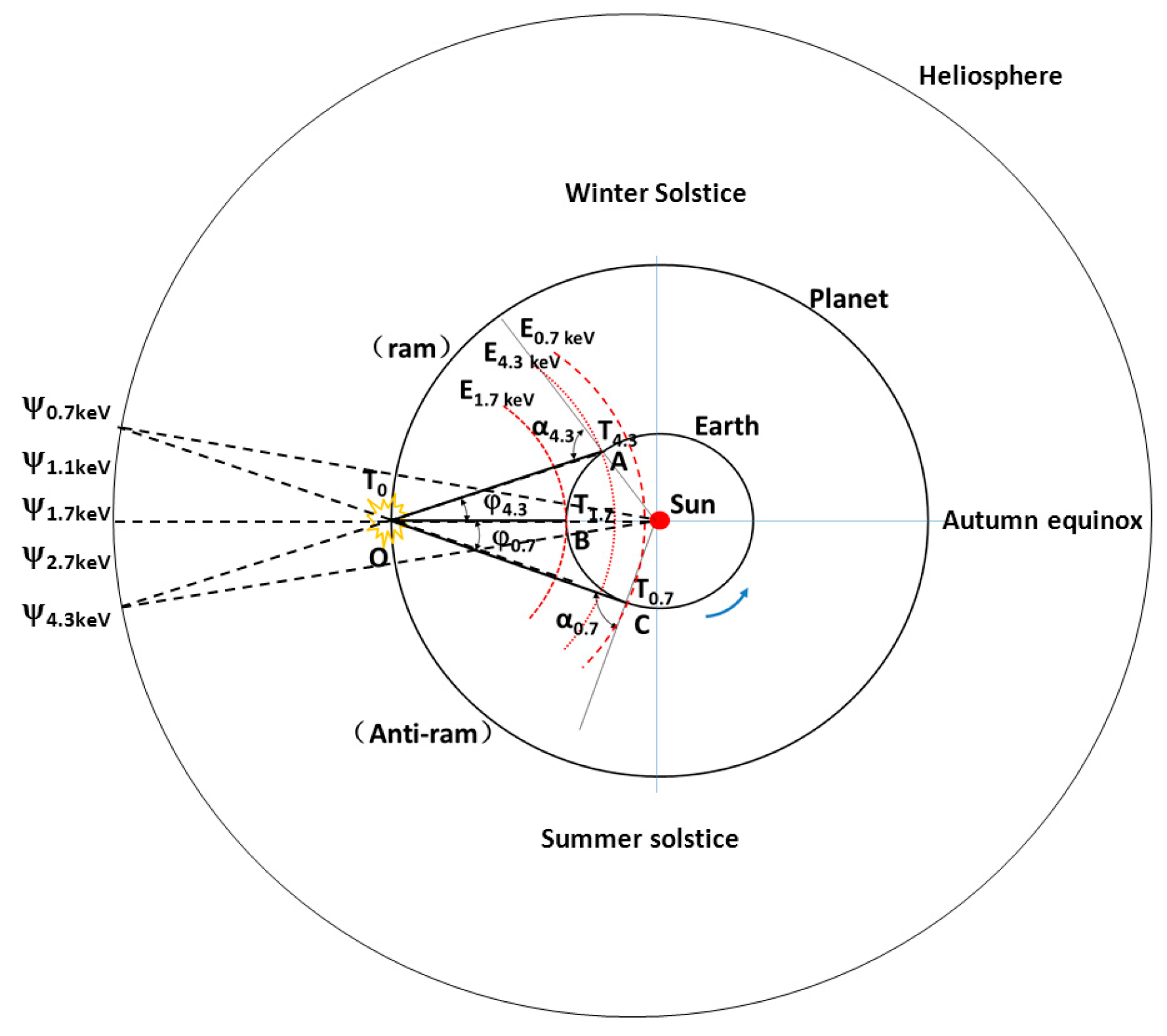
ENA emission is usually an occasional event and does not persist in a particular region all the time. Within the ecliptic plane, an Earth-size planet with a magnetosphere orbiting within the range of Jupiter (assuming an orbital radius of 7 AU) is taken as an example, shown in Figure 1: (1) At T0 (T0 = 0). The solar wind disturbance produces both the magnetic storm and ENA particle event with different energy at the vernal equinox (the ecliptic longitude of the heliosphere ψ =0°). (2) Without considering the influence of solar gravity and radiation pressure on the orbit’s deflection of the ENA particles, at the time T4.3 (T4.3= 11 days 11.19 h), the ENA imager collects the ENA particles from the ram direction with energy E = 4.3 KeV at position A of the Earth’s orbit, the observational longitude α4.3 = 187.8°, and the ecliptic longitude of the heliosphere ψ4.3kev =0.97°, the X-axis points to the sun. (3) The ENAs with energy E = 1.7 keV arrive at position B of the Earth’s orbit at the time T1.7 (T1.7 = 18 days 5.08 h) (from A to B, the payload has rotated about 6.76° along the Earth’s orbit at the ecliptic plane), and the observational longitude α1.7 = 180°, the ecliptic longitude of the heliosphere ψ1.7keV = 0°. (4) At the time T0.7 (T0.7 = 28 days 11.21 h), the ENA imager collected the ENAs with energy E = 0.7 keV from the anti-ram direction at position C of the Earth’s orbit (from B to C, the payload rotated about 10.17° along the Earth’s orbit), the observational longitude α0.7 = 168.1°, and the ecliptic longitude of the heliosphere ψ0.7keV = −1.63°. In Figure 1, ψ0.7keV, ψ1.1keV, ψ1.7keV, ψ2.7keV, and ψ4.3keV are the ENA image parallax generated by the different energy ENAs with the same ENA event. Considering the continuity of the ENA spectrum, the result of the observational ENA ribbon along the ecliptic longitude of the heliosphere is obtained. The parallax Δψ will increase slightly if the correction of the ENA’s orbit by solar gravity and radiation pressure is taken into account.
A 2D rectangular array of 0.5° × 0.5° collimation detector is adopted, and the instrument technical parameters of the ENA imaging simulation are shown in Table 2 [22], where the energy channel division refers to IBEX-Hi.
There is insufficient data to model the magnetosphere of planets other than Earth in the solar system. We used the Earth’s magnetosphere model within a particular planet’s orbit (here, the planetary orbits are symbolic) to simulate the ENA emission contribution to the 2D ENA imaging measurements as we have done in reference [22]. We quantitatively analyzed the 2D imaging parallax caused by the lag of the energy spectrum of the remote telemetry ENA imaging and studied the measurement scheme of the ENA emission source tracking in interplanetary space.
Taking the planetary magnetosphere of the Earth’s scale with an astronomical unit of 7 AU and 11 AU as an example, we simulated the ENA imaging measurement in Figure 1 with the integral time of one day considering the moderate magnetic storm of Kp = 5.
The planetary magnetosphere co-ordinate system is established in the ecliptic plane: the right-hand helical coordinate system with x axis points to the sun, and z axis points to the North Pole. According to the IBEX-Hi’s energy channel division, the co-ordinates of the ENA signals for the different energy received in the Earth’s orbit were calculated, as shown in Table 3. Suppose an Earth-sized planet has a moderate magnetic storm (Kp = 5) at position O in Figure 1, and the ENA imager on the Earth’s orbit (e.g., Lagrange 3, 4 and 5) happens to be in the specified location at a specific moment, as shown in Figure 1. Considering the energy spectral time difference, we obtained ENA simulation images in the range of Jupiter and Saturn, as shown in Figure 2.
Table 4 shows the simulated detector azimuth and longitude of the heliospheric ecliptic caused by the time-delay phenomena of the different energy channels. Considering the randomness of the ENA events and the continuity of the energy spectra, the point-like distribution of the simulated map is actually a ribbon formed by overlapping emission “nodes” along the longitude. The energy channels may overlap, and the length of the overlap is related to the duration of the solar wind disturbance. The longitude distribution range of the ENA ribbon images in the different energy channels increases with the increase of the telemetering distance. However, the heliospheric ecliptic longitude disparity (Δψ = ψ4.3keV − ψ0.7keV) of the ENA images in the different energy channels decreases with the increase of the telemetering distance. Under extreme circumstances, when the ENA signal comes from the heliospheric top of 120 AU, the longitude disparity of the ENA spectrum image decreases to 0 (Δψ = 0), theoretically.
For the same ENA emission event, the ecliptic longitude of the ENA flux peak values in the different energy channels increases with the increase of the ENA energy; that is, it moves towards the direction of the Earth’s revolution. Therefore, the spectral sequence of the longitude measured by the 2D ENA imager (decreasing longitude from high energy to low energy) is exactly opposite to the scanning sequence of IBEX-Hi (increasing longitude along the direction of revolution). This indicates that the ENA peaks of the same longitude collected by IBEX-Hi in the different energy channels are not from the same ENA source, or from the same ENA emission event. Due to time lags, if the ENA peak distribution regions of the different energy channels of IBEX-Hi are similar in longitude, this indicates that the ENA emission source is not very far from the observation position, or the ENA sustained emission time of the same source is very long.
The scale of the planetary magnetosphere is too small for AU magnitude telemetry distances, where the solid angle towards a single detector is less than a pixel, and the integral counts that last for one day do not meet the statistical requirements of ENA imaging (Table 5). If we define an “effective differential flux ()” in terms of the actual solid angle (Ωact) of the planetary magnetosphere to the detector:
where CENA is the ENA counts of the simulation detection; Integral time T = 86,400 s; ΔE (keV) is the ENA channel width (see Table 2); the actual solid angle of the planetary magnetosphere to the detector: Ωact (7 AU) =1.00674 × 10⁻⁸, Ωact (11 AU) = 3.6276 × 10⁻⁹; Effective area of the single detector Sd = 1.42 cm2. The simulation results of the average differential flux of the magnetosphere during a moderate magnetic storm (Kp = 5) in Table 5 are basically consistent with the actual measured results of the peak values of each IBEX-Hi channel [10]. The measured peak fluxes of IBEX-Hi from 0.7 to 4.3 keV were 800, 400, 140, 60, and 18 ENAs/(cm2 sr s keV), respectively.
Jupiter, located about 5.205 AU from the sun, is the largest planet in the solar system and has a very large magnetic field, about 20,000 times stronger than Earth’s at its source. Unlike Earth, Jupiter’s magnetic field is generated not by its core, but by the interaction of elements in its outer core, which is made up of liquid metal hydrogen. It is buffeted by solar wind, streams of charged particles, and magnetic fields constantly blowing from the sun. Depending on how strong the solar wind blows, Jupiter’s magnetic field can extend out as much as 3.2 million kilometers (about 52 times farther than the Earth’s magnetic field), with a magnetotail as far as Saturn’s orbit (9.576 AU). The minimum solid angle of Jupiter’s magnetosphere to the Lagrange point is about 1.046 × 10⁻⁴ (~0.583° × 0.583°), which is larger than one pixel of the ENA imager (0.5° × 0.5°). The experience of ENA imaging observation in Earth’s space shows that the enhanced ENA signal can be measured mostly when there is a large amount of kinetic energy of solar wind particles injected during geomagnetic activity [23,24,25,26]. With the differential flux measured by IBEX-Hi, at the Lagrange point for Jupiter’s distance of only one pixel (0.5° × 0.5°), the amount of kinetic energy of solar wind particles needed to be injected into Jupiter’s magnetosphere is nearly 2700 times that of the Earth’s magnetosphere during a moderate storm.
Saturn, about 9.576 AU from the sun, is the only planet whose magnetic field aligns with its axis of rotation. Saturn’s magnetic field is 17 to 34 times stronger than Earth’s and extends into Titan’s orbit, making it the flattest shape. Due to a smaller size and further distance from the Earth’s orbit, its contribution to ENA ribbon emission might be small. Uranus and Neptune have magnetic fields that are three to six times and two to eight times that of Earth, respectively, and are further from the Earth’s orbit, hence the ENA emission contribution to the ENA ribbon is negligible.
4. ENA Emission Cones Produced by Intermittent Solar Wind Ion Flow near 1 AU
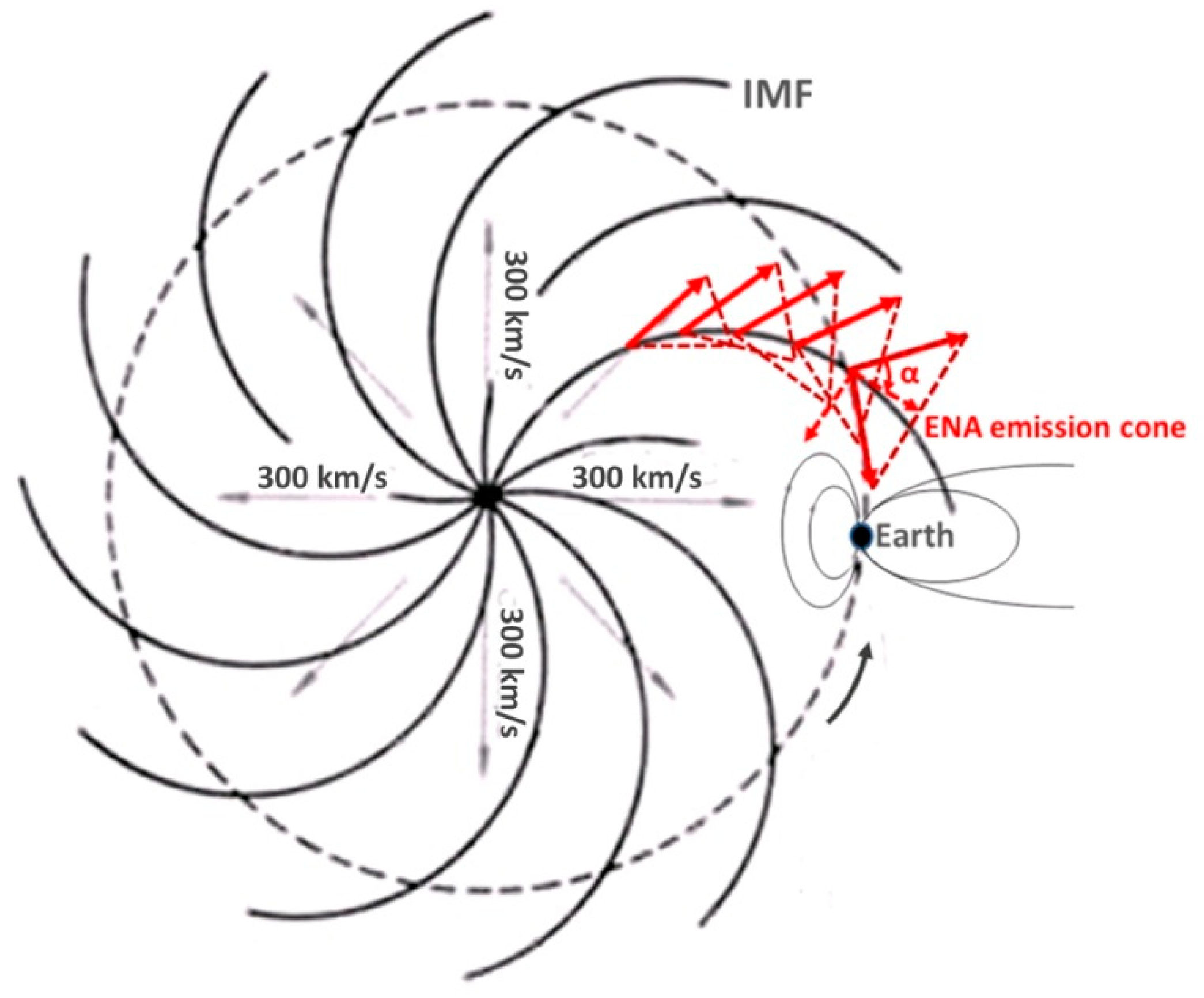
McComas et al. [17] pointed out that the possibility where multiple mechanisms coexist was not excluded. They have suggested that ENAs come from shock-accelerated pickup ions of the solar wind inside the termination shock. The ENA emission of the solar wind ions frozen in the interplanetary magnetic field (IMF) was considered to be optically thin before. The angle between the IMF (Archimedes spiral) and the radial diffusion speed of the solar wind is the maximum pitch angle α of the solar wind ions. Near the Earth’s orbit, the solar wind ion, pitch angle α ≈ 45°, exchanges charge with the neutral gas (density: N~1–10 cm3) evaporating from the Earth’s corona to form an “ENA emission cone” with a cone angle of 2α ≈ 90°, as shown in Figure 3. The inner side of the ENA emission cone is tangent to the Earth’s orbit, which may be the peak signal of the IBEX ribbon in the ram direction.
The interplanetary magnetic field (IMF) is a passive field. The spatial distribution of the solar wind ions frozen in the IMF near Earth is uneven and does not fill the entire interplanetary space. Chang ‘E-1 has repeatedly passed through the solar wind region near the lunar orbit, and the duration of each crossing is about 10s of minutes. According to the in situ measurements of Solar Wind Ion Detectors (SWID/A&B) on the boat of Chang ‘E-1 [27], the region of interplanetary space with a proton energy of ~1 keV and differential flux of 106–107 cm−2 sr−1 s−1 keV−1 was defined as Solar Wind Ion Flow (SWIF). The occurrence of SWIF is characterized by remarkable contingencies. SWIF may produce a differential flux of ENA emission:
where the collision cross-section of a hydrogen atom σpH ≈ 10−15–10−16 cm2 and the density of a hydrogen atom nH ≈ 1–10 cm−3 [28]. Ignore the helium density nHe for IBEX-Hi measurements with an ENA differential flux of 101–102 cm−2 sr−1 s−1 keV−1 and an ENA integral length of SWIF L ≈ 104–105 km. Considering the relative velocity of the satellite and solar wind (~300 km/s), the spatial scale of SWIF near Earth is similar to the estimated L value.
JENA = Jp(σpHnH + σpHenHe)L,
The differential flux maximum observed in the ram direction of IBEX-Hi is about two times that in the anti-ram direction [9]. The energy channel spectrum displacement by the Earth’s revolution speed (29.8 km/s), the purple shift or red shift, is not sufficient to reach the difference of the particle velocities between the adjacent channels (see Table 1). The distribution of the ram and anti-ram ENA ribbon patterns is also different. If we consider the ENA emission cone contribution of the solar winds and the neutral gas background (density: N~0.1–1 cm3) in interplanetary space, the ENA imager near the Lagrange point can observe this ENA emission from the ram direction perpendicular to the radial direction of the sun. The variation of the solar wind ion energy with latitude also supports the measurement results of the IBEX-Hi high-energy segment [8]. However, in the anti-ram perpendicular to the sun’s radial direction, IBEX-Hi is unable to receive signals from the ENA emission cone of the solar wind near the Earth’s orbit. As the radial distance extends outwards, the pitch angle α of the solar wind ions will soon approach ≤ 90°, and the signal of the ENA emission cone also has a chance to enter the anti-ram direction of IBEX-Hi.
“ENA ribbon” may correspond to a global distribution of SWIFs generated by the interaction of fast and slow solar winds [29]. Those SWIFs will form a tailward distribution loop under the interstellar wind pressure.
5. Conclusions
We suspect that the magnetic structure of the heliopause pickup solar wind ions is able to form a huge ENA emission wall which enables measurements of the ENA ribbon at a distance from the Earth’s orbit. The ENA emission cone of the solar wind in interplanetary space may be the main ENA emission source of the ENA ribbon, especially the peak signal of the ribbon. We propose that there exists a tailward SWIF distribution loop in interplanetary space. The ENA differential flux generated by the “ENA emission cone” of the solar wind ion stream near 1 AU is of the same order of magnitude as the peak signal of the ENA ribbon.
By simulating ENA imaging of the magnetosphere of distant planets, we demonstrate how to measure the location of ENA emission sources using ENA signal parallax caused by energy spectrum delay. In the solar system, except for Jupiter, the magnetospheres of other planets are too small to meet the statistical requirements of ENA ribbon imaging. Jupiter’s magnetosphere itself, orbiting near the ecliptic, has a solid angle of only about 0.5° × 0.5° from the Earth’s orbit. This is neither sufficient to produce the emission “knots” strung together in the ENA ribbon scanned by IBEX = Hi (6°×6° per pixel), nor does it explain the sources of the high-latitude signals in the spectrum.
The Lagrange points (L5, L4, or L3) within the plane of the Earth’s orbit around the sun, with a clean emission environment and facing the zenith, avoid interference from the ENA emission from the Earth’s magnetosphere. It is the ideal location for the ENA ribbon measurement, as the Earth orbits, that we proposed in Figure 1. The proposed 2D ENA imaging measurement can collect the time lag and disparity of the peak ENA signals in the different energy channels to confirm the spatial location of the ENA emission sources and further investigate the origin of the ENA ribbon. The azimuth variation of signals in the 2D ENA image measured at the Lagrange points (L5, L4, or L3), from the ram to anti-ram direction, will be the key data to support and identify the location of the ENA emission source.
Author Contributions
Conceptualization, L.L.; methodology, L.L.; software, L.L.; validation, L.L.; formal analysis, L.L.; investigation, L.L.; resources, Q.Y., S.J. and Y.C.; data curation, L.L.; writing—original draft preparation, L.L.; writing—review and editing, L.L.; visualization, L.L.; supervision, L.L.; project administration, Q.Y., S.J. and Y.C.; funding acquisition, Q.Y. All authors have read and agreed to the published version of the manuscript.
Funding
National Key R&D Program of China (Grant No. 2020YFE0202100), National Mission/Other National Mission: Research on Key Technologies of the Outer Heliospheric Space Exploration System (Grant No. Y91 Z100102) and National Mission/National Major Science and Technology Project: CE-7 Relay Satellite Display Neutral Atom Imager (Grant No. E16504 B31S).
Institutional Review Board Statement
Not applicable.
Informed Consent Statement
Not applicable.
Acknowledgments
This study was Supported by National Key R&D Program of China (Grant No. 2020YFE0202100), National Mission/Other National Mission: Research on Key Technologies of the Outer Heliospheric Space Exploration System (Grant No. Y91 Z100102) and National Mission/National Major Science and Technology Project: CE-7 Relay Satellite Display Neutral Atom Imager (Grant No. E16504 B31 S).
Conflicts of Interest
The authors declare no conflict of interest.
References
- McComas, D.J.; Alegrini, F.; Bochsler, P.; Bzowski, M.; Christian, E.R.; Crew, G.B.; Demajistre, R.; Fahr, H.; Fichtner, H.; Frisch, P.C.; et al. Global observations of the interstellar interaction from the Interstellar Boundary Explorer (IBEX). Science 2009, 326, 959–962. [Google Scholar] [CrossRef] [PubMed]
- Puselier, S.A.; Allegrini, F.; Funsten, H.O.; Ghielmetti, A.G.; Heirtzler, D.; Kucharek, H.; Lennartsson, O.W.; Mccomas, D.J.; Mobius, E.; Moore, T.E.; et al. Width and variation of the ENA flux ribbon observed by Interstellar Boundary Explorer. Science 2009, 326, 962–964. [Google Scholar] [CrossRef]
- Krimigis, S.M.; Mitchell, D.G.; Roelof, E.C.; Hsieh, K.C.; McComas, D.J. Imaging the intersection of the heliosphere with the interstellar medium from Saturn with Cassini. Science 2009, 326, 971–973. [Google Scholar] [CrossRef] [PubMed] [Green Version]
- McComas, D.J.; Funsten, H.O.; Fuselier, S.A.; Lewis, W.S.; Mobius, E.; Schwadron, N.A. IBEX observations of heliospheric energetic neutral atoms: Current understanding and futured direction. Geophys. Res. Lett. 2011, 38, L18101–L18109. [Google Scholar] [CrossRef]
- Swaczyna, P.; Bzowski, M.; Christian, E.R.; Funsten, H.O.; McComas, D.J.; Schwadron, N.A. Distance to the IBEX ribbon source inferred from parallax. Astrophys. J. 2016, 823, 11. [Google Scholar] [CrossRef] [Green Version]
- McComas, D.J.; Zirnstein, E.J.; Bzowski, M.; Dayeh, M.A.; Funsten, H.O.; Fuselier, S.A.; Janzen, P.H.; Kubiak, M.A.; Kucharek, H.; Möbius, E.; et al. Seven Years of Imaging the Global Heliosphere with IBEX. Astrophys. J. Suppl. 2017, 229, 32. [Google Scholar] [CrossRef] [Green Version]
- McComas, D.J.; Bzowski, M.; Dayeh, M.A.; DeMajistre, R.; Funsten, H.O.; Janzen, P.H.; Kowalska, I.; Kubiak, M.A.; Schwadron, N.A.; Sokół, J.M.; et al. Solar Cycle of Imaging the Global Heliosphere: Interstellar Boundary Explorer (IBEX) Observations from 2009–2019. Astrophys. J. Suppl. 2020, 248, 33. [Google Scholar] [CrossRef]
- Zirnstein, E.J.; Heerikhuisen, J.; Mccomas, D.J. Structure of the interstellar boundary explorer ribbon from secondary charge-exchange at the solar-interstellar interface. Astrophys. J. 2015, 804, L22. [Google Scholar] [CrossRef]
- Funsten, H.O.; Allegrini, F.; Crew, G.B.; Demajistre, R.; Frisch, P.C.; Fuselier, S.A.; Gruntman, M.; Janzen, P.; Mccomas, D.J.; Mobius, E.; et al. Structures and spectral variations of the outer heliosphere in IBEX energetic neutral atom maps. Science 2009, 326, 964–966. [Google Scholar] [CrossRef]
- McComas, D.J.; Dayeh, M.A.; Allegrini, F.; Bzowski, M.; DeMajistre, R.; Fujiki, K.; Funsten, H.O.; Fuselier, S.A.; Gruntman, M.; Janzen, P.H.; et al. The frist three years of IBEX observations and our evolving heliosphere. Astrophys. J. Suppl. 2012, 203, 1–36. [Google Scholar] [CrossRef]
- Schwadron, N.A.; Bzowski, M.; Crew, G.B.; Gruntman, M.; Fahr, H.; Fichtner, H.; Frisch, P.C.; Funsten, H.O.; Fuselier, S.; Heerikhuisen, J.; et al. Comparison of Interstellar Boundary Explorer observations with 3D global heliospheric models. Science 2009, 326, 966–968. [Google Scholar] [CrossRef] [PubMed]
- Mccomas, D.J.; Lewis, W.S.; Schwadron, N.A. IBEX’s Enigmatic Ribbon in the sky and its many possible sources. Rev. Geophys. 2014, 52, 118–155. [Google Scholar] [CrossRef]
- Bertaux, J.L.; Blamont, J.E. Evidence for a source of an extraterrestrial hydrogen lyman-alpha emission. Astron. Astrophys. 1971, 11, 200–217. [Google Scholar]
- Fisk, L.A.; Kozlovsky, B.; Ramaty, R. An interpretation of the observed oxygen and nitrogen enhancements in low-energy cosmic rays. Astrophys. J. 1974, 190, L35–L37. [Google Scholar] [CrossRef] [Green Version]
- Dialynas, K.; Krimigis, S.M.; Mitchell, D.G.; Decker, R.B.; Roelof, E.C. The bubble-like shape of the heliosphere observed by Voyager and Cassini. Nat. Astron. 2006, 1, 0115. [Google Scholar] [CrossRef]
- Wang, L.; Lin, R.; Larson, D.; Luhmann, J.G. Domination of heliosheath pressure by shock-accelerated pickup ions from observations of neutral atoms. Nature 2008, 454, 81–83. [Google Scholar] [CrossRef] [PubMed]
- McComas, D.J.; Bzowski, M.; Frisch, P.; Crew, G.B.; Dayeh, M.A.; DeMajistre, R.; Funsten, H.O.; Fuselier, S.A.; Gruntman, M.; Janzen, P.; et al. Evolving outer heliosphere: Large-scale stability and time variations observed by the Interstellar Boundary Explorer. J. Geophys. Res. 2010, 115, A09113. [Google Scholar] [CrossRef] [Green Version]
- Priscilla, C.F.; Redfield, S.; Slavin, J.D. The Interstellar Medium Surrounding the Sun. Ann. Rev. Astron. Astrophys. 2011, 49, 237–279. [Google Scholar]
- Witte, M. Kinetic parameters of interstellar neutral helium. Review of results obtained during one solar cycle with the Ulysses/GAS-instrument. Astron. Astrophys. 2004, 426, 835–844. [Google Scholar] [CrossRef]
- Mobius, E.; Bochsler, P.; Bzowski, M.; Crew, G.B.; Funsten, H.O.; Fuselier, S.A.; Ghielmetti, A.; Heirtzler, D.; Izmodenov, V.V.; Kubiak, M.; et al. Direct observations of interstellar H, He, and O by the interstellar Boundary Explorer. Science 2009, 326, 969–971. [Google Scholar] [CrossRef]
- Luhmann, J.G.; Curtis, D.W.; Schroeder, P.; McCauley, J.; Lin, R.P.; Larson, D.E.; Bale, S.D.; Sauvaud, J.-A.; Aoustin, C.; Mewaldt, R.A.; et al. STEREO IMPACT investigation goals, measurements, and data products overview. Space Sci. Rev. 2008, 136, 117–184. [Google Scholar] [CrossRef] [Green Version]
- Lu, L.; Yu, Q.L.; Zhou, P.; Zhang, X.; Zhang, X.G.; Wang, X.Y.; Chang, Y. Simulation study of the energetic neutral atom (ENA) imaging monitoring of the geomagnetosphere on a lunar base. Sol. Terr. Phys. 2021, 7, 3–10. [Google Scholar] [CrossRef]
- Roelof, E.C. Energetic neutral atom image of a storm-time ring current. Geophys. Res. Lett. 1987, 14, 652–655. [Google Scholar] [CrossRef]
- Brandt, P.C.; Demajistre, R.; Roelof, E.C.; Ohtani, S.; Mitchell, D.G.; Mende, S. IMAGE/high-energy energetic neutral atom: Global energetic neutral atom imaging of the plasma sheet and ring current during substorms. J. Geophys. Res. 2002, 107, SMP21-1–SMP21-13. [Google Scholar] [CrossRef]
- McComas, D.J.; Buzulukova, N.; Connors, M.G.; Dayeh, M.A.; Goldstein, J.; Funsten, H.O.; Fuselier, S.; Schwadron, N.A.; Valek, P. Two wideangle imaging neutral-atom spectrometers and interstellar boundary explorer energetic neutral atom imaging of the 5 April 2010 substorm. J. Geophys. Res. 2012, 117, A03225. [Google Scholar]
- Lu, L.; McKenna-Lawlor, S.; Cao, J.B.; Kudela, K.; Balaz, J. The causal sequence investigation of the ring current ion-flux increasing and the magnetotail ion injection during a major storm. Sci. China Earth Sci. 2016, 59, 129–144. [Google Scholar] [CrossRef]
- Hong, S.; Tian, L.C.; Yang, S.S. Analysis of data obtained by the solar wind ion detector onboard the Chang’E-1 Lunar orbiter. Acta Phys. Sin. 2014, 63, 069601. [Google Scholar] [CrossRef]
- Lu, L.; Mckenna-Lawlor, S.; Barabash, S.; Balaz, J.; Liu, Z.X.; Shen, C.; Cao, J.B.; Tang, C.L. Iterative inversion of global magnetospheric information from energy neutral atom (ENA) images recorded by the TC-2/NUADU instrument. Sci. China Technol. Sci. 2008, 51, 1731–1744. [Google Scholar] [CrossRef]
- Xiaojun, X.; Fengsi, W.; Xueshang, F. Characteristics of reconnection diffusion region in the solar wind. Chin. J. Space Sci. 2012, 32, 778–784. [Google Scholar]
Figure 1.
Schematic diagram of planetary magnetosphere ENA image measurements at the Lagrange point.
Figure 1.
Schematic diagram of planetary magnetosphere ENA image measurements at the Lagrange point.

Figure 2.
Simulated ENA images of 1-day integral at the Lagrange point for the planetary magnetosphere with heliocentric distances of 7 AU (a) and 11 AU (b).
Figure 2.
Simulated ENA images of 1-day integral at the Lagrange point for the planetary magnetosphere with heliocentric distances of 7 AU (a) and 11 AU (b).

Figure 3.
The interplanetary magnetic field lines and the corresponding ENA emission cone (marked red) near 1 AU.
Figure 3.
The interplanetary magnetic field lines and the corresponding ENA emission cone (marked red) near 1 AU.


Table 1.
The velocities and time lags of hydrogen atoms traveling 1 AU at different energies.
| E (KeV) | V (km/s) | T (h) | ∆T (h) |
|---|---|---|---|
| 0.7 | 366.0509 | 113.5222264 | 22.962820341 17.712318465 15.043505926 11.999682392 |
| 1.1 | 458.8691 | 90.559406059 | |
| 1.7 | 570.4491 | 72.847087594 | |
| 2.7 | 718.9097 | 57.803581668 | |
| 4.3 | 907.2493 | 45.803899276 |
Table 2.
Instrument design parameters for the imaging simulation.
| Atomic Species | H,O (Simulation: H) | ||||
|---|---|---|---|---|---|
| Energy range and channels | 0.4–10 keV (simulation: 0.4–5 keV) | ||||
| 0.4–1 keV | 0.8–1.4 keV | 1.3–2.1 keV | 2.2–3.2 keV | 3.7–4.9 keV | |
| Field of view | 30° × 30° (simulation: 20° × 40°) | ||||
| Angle resolution | ≤0.5° (simulation: 0.5° × 0.5°) | ||||
| Geometric factor | Single detector: 10−4 cm 2 sr; (simulation: 20 × 40 ≈ 0.0865) | ||||
| Sampling period | Simulation: 1 days | ||||
| Element numbers | Simulation: 30 (latitude) × 60 (longitude) × 18 (L value) = 32,400 | ||||
Table 3.
Position parameters of ENA imaging simulations.
| Scope | E (keV) | Latitude (°) | Longitude (°) | X (AU) | Y (AU) | Z (AU) |
|---|---|---|---|---|---|---|
| 7 (AU) | 0.7 | 90 | −169.83 | 6.015708724 | −0.176552213 | 0.0 |
| 1.1 | 90 | −175.63 | 6.002904555 | −0.076162156 | 0.0 | |
| 1.7 | 90 | 180.00 | 6.0 | 0.0 | 0.0 | |
| 2.7 | 90 | 176.29 | 6.00209566 | 0.064706476 | 0.0 | |
| 4.3 | 90 | 173.24 | 6.006954127 | 0.11772805 | 0.0 | |
| 11 (AU) | 0.7 | 90 | −163.39 | 10.0417223 | −0.285838896 | 0.0 |
| 1.1 | 90 | −172.72 | 10.00805905 | −0.12670105 | 0.0 | |
| 1.7 | 90 | 180.00 | 10.0 | 0.0 | 0.0 | |
| 2.7 | 90 | 173.82 | 10.00581516 | 0.107687028 | 0.0 | |
| 4.3 | 90 | 168.89 | 10.01876114 | 0.192754885 | 0.0 |
Table 4.
FOV longitude simulation results for different energy channels.
| E (keV) | FOV Azimuth (°) | Ecliptic Longitude (°) | ||
|---|---|---|---|---|
| 7 (AU) | 11 (AU) | 7 (AU) | 11 (AU) | |
| 0.7 | 168.1 | 161.9 | −1.63 | −1.35 |
| 1.1 | 174.7 | 172.1 | −0.72 | −0.59 |
| 1.7 | 180.0 | 180.0 | 0.00 | 0.00 |
| 2.7 | 184.5 | 186.7 | 0.61 | 0.50 |
| 4.3 | 187.8 | 192.1 | 0.97 | 0.90 |
Table 5.
Simulation results of ENA counts and effective differential fluxes.
| E (keV) | ENA Counts | Effective Differential Flux: ENAs/(cm2 sr s kev) | ||
|---|---|---|---|---|
| 7 (AU) | 11 (AU) | 7 (AU) | 11 (AU) | |
| 0.7 | 0.8037 | 0.2991 | 941.9 | 978.2 |
| 1.1 | 0.3949 | 0.1366 | 294.5 | 298.3 |
| 1.7 | 0.3547 | 0.1279 | 171.1 | 171.4 |
| 2.7 | 0.1815 | 0.0661 | 55.1 | 55.7 |
| 4.3 | 0.1061 | 0.0397 | 24.2 | 21.0 |
Publisher’s Note: MDPI stays neutral with regard to jurisdictional claims in published maps and institutional affiliations. |
© 2022 by the authors. Licensee MDPI, Basel, Switzerland. This article is an open access article distributed under the terms and conditions of the Creative Commons Attribution (CC BY) license (https://creativecommons.org/licenses/by/4.0/).
Share and Cite
MDPI and ACS Style
Lu, L.; Yu, Q.; Jia, S.; Chang, Y. Energetic Neutral Atom (ENA) Imaging Simulation of the Distant Planetary Magnetosphere and ENA Emission Discussion of the Solar Wind. Astronomy 2022, 1, 235-245. https://doi.org/10.3390/astronomy1030013
AMA Style
Lu L, Yu Q, Jia S, Chang Y. Energetic Neutral Atom (ENA) Imaging Simulation of the Distant Planetary Magnetosphere and ENA Emission Discussion of the Solar Wind. Astronomy. 2022; 1(3):235-245. https://doi.org/10.3390/astronomy1030013
Chicago/Turabian StyleLu, Li, Qinglong Yu, Shuai Jia, and Yuan Chang. 2022. "Energetic Neutral Atom (ENA) Imaging Simulation of the Distant Planetary Magnetosphere and ENA Emission Discussion of the Solar Wind" Astronomy 1, no. 3: 235-245. https://doi.org/10.3390/astronomy1030013