Wind Speed Forecast for Sudan Using the Two-Parameter Weibull Distribution: The Case of Khartoum City

Abstract

In this quick study, we estimated the Weibull distribution’s parameters using wind data collected between March 2017 and January 2018 using a twelve-meter mast meteorological station on the grounds of the National Energy Research Center in Khartoum. In order to quantify these descriptors, we relied on analytical and stochastic methods, subsequently enabling specialists from researchers, engineers, decision-makers, and policymakers to apprehend the wind characteristics in the vicinity. Hence, the computed scale and shape parameters were provided, in which the Firefly algorithm (FA) resulted in the most accuracy in terms of the coefficient of determination, which equaled 0.999, which we considered logical due to the observed nonlinearity in the wind speed numbers. On the contrary, the energy pattern factor method had the worst prediction capability depending on several goodness-of-fit metrics. This concise work is unique because it is the first to use data from Sudan to forecast local wind speeds using artificial intelligence algorithms, particularly the FA technique, which is widely used in solar photovoltaic modeling. Additionally, since classic estimating approaches act differently spatially, evaluating their efficacy becomes innovative, which was accomplished here. On a similar note, a weighted-average wind speed was found to equal $4.98 \mathrm{m}/\mathrm{s}$ and the FA average wind speed was $3.73 \mathrm{m}/\mathrm{s}$, while the rose diagram indicated that most winds with potential energy equivalent to $3 \mathrm{m}/\mathrm{s}$ or more blow from the north.

1. Introduction

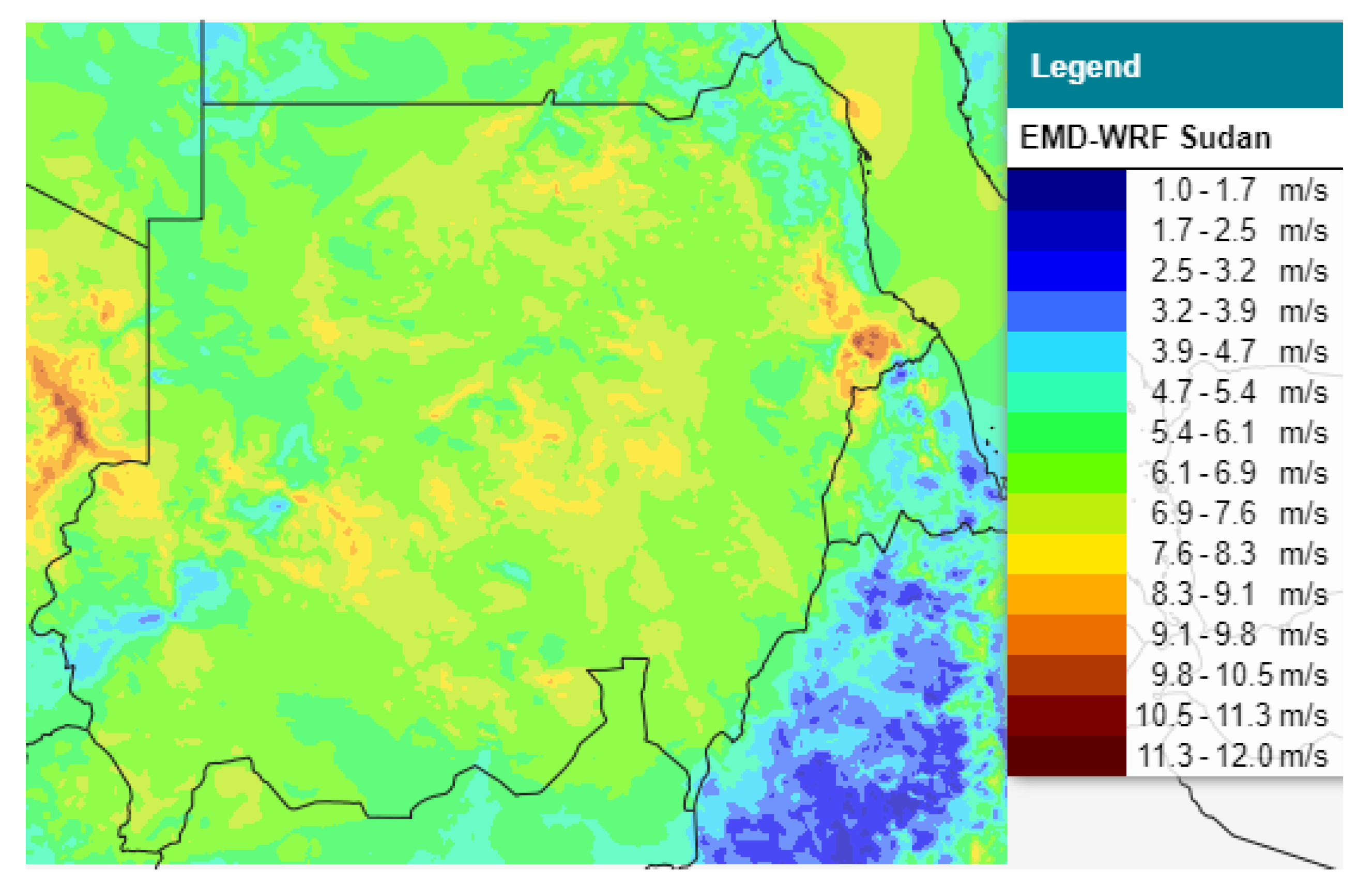
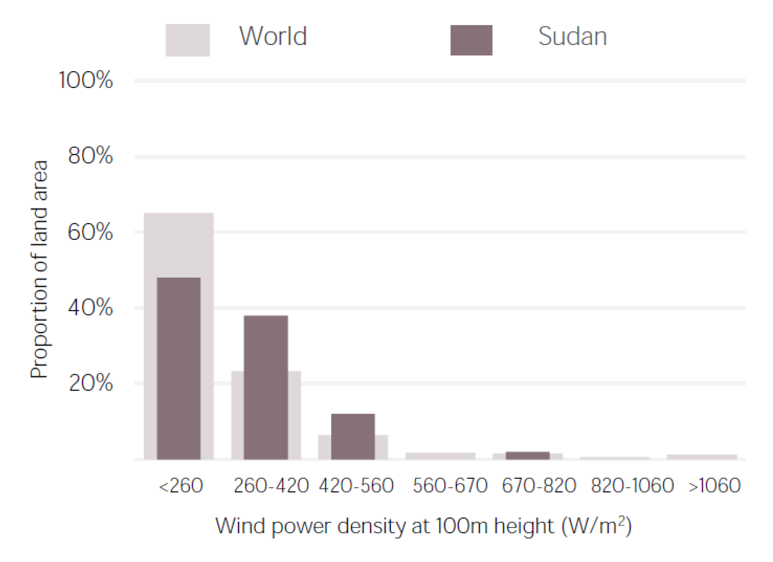
Sudan is an enormous reservoir of renewable energy resources, with an evident annual wind energy yield, which is verified by GIS analysis [1], as shown in in Figure 1 [2,3] and Figure 2 [4]. The government-endorsed plans that encourage the switch to clean energy generation were included in the 2015 Intended Nationally Determined Contribution (INDC) declaration that was presented to the United Nations Framework Convention on Climate Change (UNFCCC). Among them, 1000 MW_p of grid-connected wind power plants is planned to be constructed in high-potential regions [5]. In 2021, the country witnessed the arrival of the first wind turbine, which will have its electricity generation fed into the national network serving 14,000 people, and has already been installed in Dongola, a rich in wind energy northern city [6].

The Weibull distribution is the most commonly used statistical distribution to model wind speed [7,8,9,10,11,12,13,14,15], which served this purpose for the first time in the late 1970s. It then established many wind energy regulations worldwide and modeled software, such as WASP and HOMER [16]. The two parameters of the Weibull distribution are well-known for being straightforward and fitting the actual wind speed readings perfectly. Hence, if these two parameters are accurately predicted, the Weibull-based forecasting model will represent the exact wind speed variations [17,18]. The work of [19] depended on the Weibull distribution to obtain wind characteristics in the Alaçatı region, Turkey, and found that its shape and scale parameters equal 2.05 and 9.16, respectively. Additionally, the mean wind speed based on the dataset was $8.11 \mathrm{m}/\mathrm{s}$. [10]. They estimated the same distribution parameters using different analytical methods and compared them with the results of other parametric and non-parametric models. In Pakistan, ref. [11] used six analytical estimation methods to identify the shape and scale estimates of the Weibull distribution and accordingly obtained an average wind speed range from $2.9 \mathrm{to} 4 \mathrm{m}/\mathrm{s}$ for different weather mast heights. In Sudan, [20] estimated the annual average wind speeds and their corresponding Weibull shape parameters at a 10 m height.

Table 1. Wind energy potential for different cities in Sudan. Adapted with permission from Ref. [20]. 2008, Elsevier.

City	Altitude (m)	Annual Wind Speed Based on Weibull Distribution (m/s)	Shape Parameter (k)
Abu Na’ama	445	3.1	2.2
Atbara	345	4.2	1.75
El Fasher	733	3.4	1.15
El Geneina	805	3.1	1.9
El Obeid	570	3.4	1.9
Karima	250	4.7	1.7
Kassala	500	4	1.95
Khartoum	380	4.8	1.9
Kosti	380	4	1.8
Port Sudan	5	5	1.6
Shambat 1	380	4.8	2.1
Wadi Halfa	190	4.6	1.8
Wad Madani	405	4.8	1.8

¹ Shambat is a station within Khartoum North city.

presents the mentioned estimates for major cities in the country.

The wind speed prediction models provide the information needed for industry development [21]. There are four main modeling techniques. (1) Physical models show better forecasting performance with long-term data; still, the precision is low. Still, suppose the resolution is high enough, and the initialization is perfect. In that case, the accuracy can be increased. (2) Statistical models include the conventional model that relies on famous probability distributions, such as Weibull, but with a limited capacity in front of nonlinear wind speed data. (3) Third, spatial algorithms, which require a large amount of information. (4) Lastly, artificial intelligence or metaheuristic algorithms, which are gaining more popularity, especially with nonlinear data [21,22,23,24,25,26,27,28,29,30,31].

Statistical models or analytical methods are widely used to extract the parameters of the Weibull distribution [12,32]. Among these techniques, the most popular ones are the maximum likelihood method (MLM), the least square method (LSM), the method of moment (MOM), and the graphical method (GM) [15]. Additionally, the metaheuristics or stochastic processes, mainly swarm intelligence algorithms, are successively used in the literature to evaluate the wind speed Weibull parameters, including the particle swarm optimization, Cuckoo search, Gray wolf algorithm, Firefly algorithm (FA), Ant Colony optimization, and many others [33]. Since FA was put forward in this study, we have to mention that many researchers developed multiple variants of FA and applied them to estimate the parameters of the Weibull distribution effectively. Ref. [34] hybridized the FA with the support vector machine method to obtain a novel, efficient way for Weibull parameter estimation. Ref. [35] used a hybrid technique containing the FA and a back-propagation neural network to evaluate the Weibull distribution parameters for wind data in China, yielding a better prediction performance.

To link points together, our work here targets utilizing several analytical methods in addition to the FA to estimate the parameters of the Weibull distribution for the wind speed data collected in Khartoum. The importance of the city as the country’s capital and the availability of the research means from meteorological stations that save long-term data and the suitable equipment made us focus our attention on this region to help us build a model or a mathematical template that will guide similar future work for the rest of the country. The novelty in this work lies in using the FA with wind speed data in Sudan and the Weibull distribution, and then comparing the results with conventional estimation methods whose quality varies location-wise. For instance, the graphical way showed a good performance, while it has proven ineffectiveness in analyzing the data in some areas in the Republic of Korea, as claimed by [36]. We placed particular attention to the FA methodology here because if we want to obtain a powerful Weibull-based forecasting model, an accurate estimation of the shape and scale parameters is of paramount importance, and this accuracy is only obtained through stochastic algorithms, precisely the swarm-intelligence set of techniques that the FA methods belong to. Accordingly, the significance of this study is reflected in forming a solid foundation for wind speed forecasting, which will comply with different sites within the surrounding area and in a larger circle involving the whole country.

Therefore, the rest of this article is organized as follows. Section 2 presents the experimental setup, which sheds information on the meteorological mast station system, and Section 3 outlines the analysis methodology, including data filtering, missing data imputation, Weibull distribution description, parameter estimation techniques, and goodness-of-fit metrics. Section 4 delivers and discusses the results, and Section 5 concludes.

2. Experimental Setup

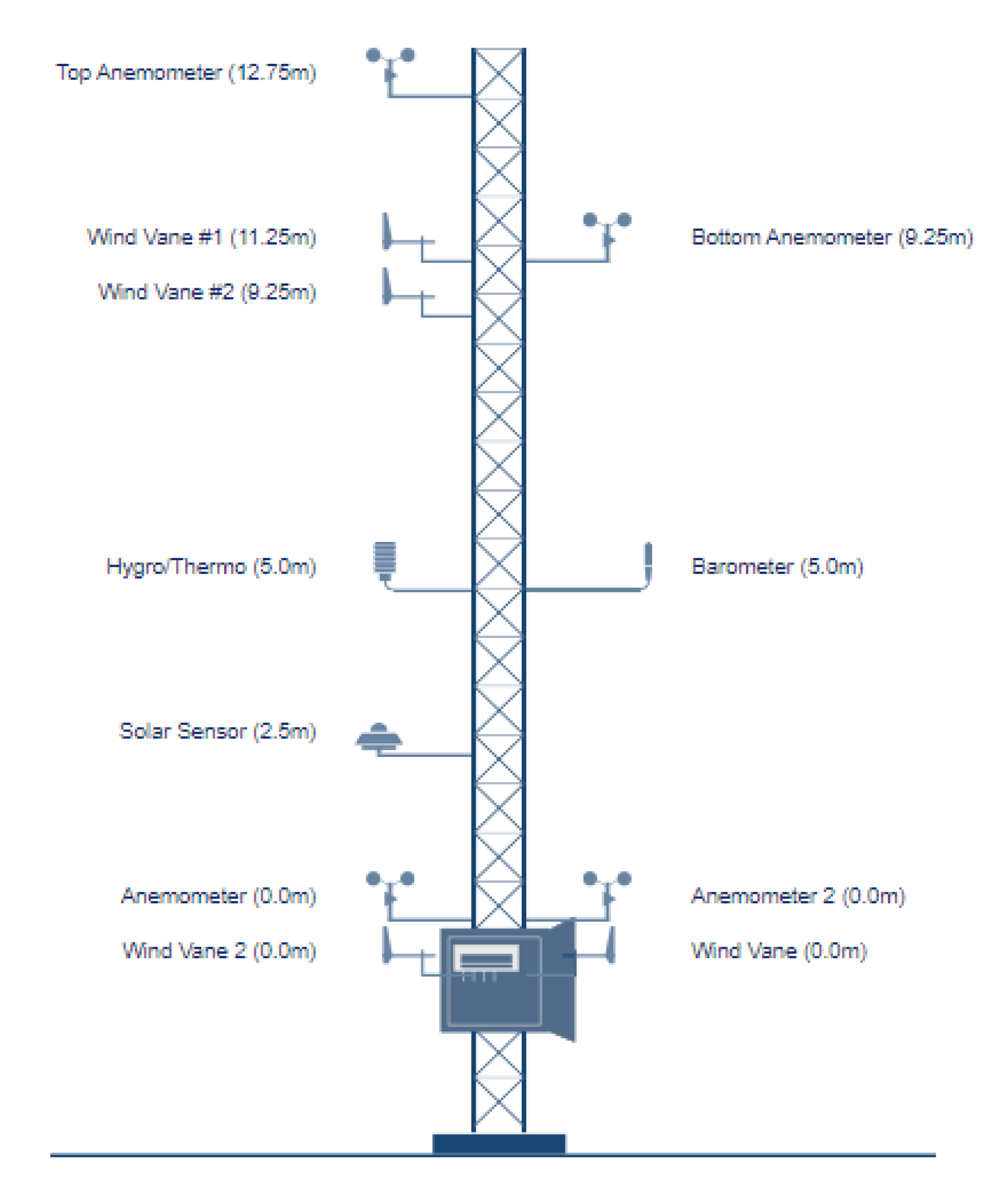
The measurement tower from which the data were taken is located inside the National Energy Research Center (NERC) campus in the Soba suburb, Khartoum, and has a $12.75 \mathrm{m}$ wind monitoring tower. At the top of the tower, a first anemometer, which measures wind speed, is fixed. Right beneath it, a wind vane that detects the wind direction is placed at $11.25 \mathrm{m}$. Below the wind vane at $9.25 \mathrm{m}$, a second anemometer is fixed, which provides a separate measurement for the wind speed. Additionally, there is a second wind vane at $9.20 \mathrm{m}$, reading another measurement for wind direction.

A barometer, an air pressure measuring device, and a thermocouple sensor are placed at $5.0 \mathrm{m}$. Moreover, a hygrometer is placed at the same height to measure the water content in the air (i.e., relative humidity). Finally, a pyranometer is connected to the tower at $2.5 \mathrm{m}$.

All the sensors or measuring devices are connected to a data acquisition system (Model: Meteo-40L, manufactured by Ammonit (Ammonit Measurement GmbH, Berlin, Germany) or data logger, in which the data are continuously collected at a sampling rate of $1 \mathrm{Hz}$ or higher. Each sensor measures and records its relevant reading once in a minute or less, and for every 10 min, the data logger saves the minimum, maximum, mean, and standard deviation of the set of measurements. It is worth mentioning that the analysis depended on retrieved data that belongs to the anemometer and wind vane set at a height of $12.7 \mathrm{m}$. Figure 3 and Figure 4 show a schematic diagram and picture of the wind mast station within the NERC premises.

3. Analysis Methodology

3.1. Data Filtering

Filtering is the process of defining, identifying, and fixing data flaws to lessen their effect [37]. In the restored readings from the mast data logger, we discovered error codes in the form of negative wind speeds, which were successively removed, leaving behind blank spaces or empty data fields. Figure 5 displays the ten-minute interval time series graph between 18 March 2017 and 30 January 2018, and Figure 6 illustrates the same data as a frequency histogram that includes the normal curve.

3.2. Missing Data Imputation

Missing data methods either discard data using complete and available case analysis techniques, also known as likewise and pairwise deletion [38], or retain all data using single and multiple imputation methods [39]. In our analysis, we used the single mean imputation approach seeking simplicity, as we have less than 0.05% missing data, though in general, the single imputation methods generate filled-in values infused with standard errors, causing bias in the sample [40]. However, we defend our choice by claiming that almost a trivial part of the data are missing if we consider the 5% missingness threshold over which rigorous imputation methods should be used [41].

3.3. Weibull Distribution

The two-parameter Weibull distribution best fits the wind speed data [42]. The probability density function of this distribution is given in Equation (1), the cumulative density function is provided in Equation (2) [43,44], and the mean and the variance are given in Equations (3) and (4), respectively [45]. Figure 7 and Figure 8 show graphs of the typical Weibull density functions [43].

$$f\left(V\right)=\frac{k}{c}{\left(\frac{V}{c}\right)}^{k-1}{e}^{-{\left(\frac{V}{c}\right)}^k}$$

(1)

where $V\ge 0$ is the wind speed.

$$F\left(V\right)=1-e^{-{\left(\frac{V}{c}\right)}^k}$$

(2)

where $V\ge 0$.

$$\mu =c\mathsf{\Gamma }\left(1+\frac{1}{k}\right).$$

(3)

$${\sigma }^2=c^2\left[\mathsf{\Gamma }\left(1+\frac{2}{k}\right)-{\mathsf{\Gamma }}^2\left(1+\frac{1}{k}\right)\right]$$

(4)

3.4. Parameter Estimation

The parameter estimation concept depends on the availability of measured data to statistically approximate the parameter value. The well-known estimation methods could be grouped into analytical, numerical iterative, and stochastic methods, which perfectly fit nonlinear models [46].

3.4.1. Analytical Methods

Energy Pattern Factor Method

The Energy pattern factor method (EPFM) estimates the scale and shape parameters of the Weibull distribution using Equations (5)–(7) [47].

$$\widehat{k}=1+\frac{3.69}{E_{pf}^2}$$

(5)

$$\widehat{c}={\left(\frac{1}{n}{\displaystyle \sum }_{i=1}^n{v}_i^{\widehat{k}}\right)}^{\raisebox{1ex}{$1$}\!\left/ \!\raisebox{-1ex}{$\widehat{k}$}\right.}$$

(6)

$$E_{pf}=\frac{\frac{1}{n}{{\displaystyle \sum }}_{i=1}^n{v}_i^3}{{\left(\frac{1}{n}{{\displaystyle \sum }}_{i=1}^n{v}_i\right)}^3}$$

(7)

Graphical Method

We chose to use the graphical method (GM) to estimate the scale and shape parameters, as this method is the most common one with reliable results [43,48,49]. Equations (8)–(10) present the estimators’ equations obtained by applying the natural logarithm transformation to Equation (2) to find the straight-line formula.

$$\ln \left[-\ln \left(1-F\left(V\right)\right)\right]=\widehat{k}\ln v_i-\widehat{k}\ln \widehat{c}$$

(8)

$$-\widehat{k}\ln \widehat{c}=y intercept$$

(9)

$$\widehat{k}=slope$$

(10)

where $F\left(V\right)$ is given in Equation (2).

Method of Moments

The method of moments (MOM) estimates the scale and shape parameters depending on Equations (11) and (12) [45,50].

$$\widehat{k}={\left(\frac{\sigma }{\mu }\right)}^{-1.091}$$

(11)

$$\widehat{c}=\frac{\mu }{\mathsf{\Gamma }\left(1+\frac{1}{\widehat{k}}\right)}$$

(12)

Least Square Method

The least square method (LSM) is an analytical technique to estimate the scale and shape parameters of the Weibull distribution [45,50], employing Equations (13) and (14) [51,52].

$$\widehat{k}=\frac{\left\{n{{\displaystyle \sum }}_{i=1}^n\left(ln{v}_i\right)·\left(\ln \left\{\ln \left[\frac{1}{\left(1-\frac{i}{n+1}\right)}\right]\right\}\right)\right\}-\left\{{{\displaystyle \sum }}_{i=1}^n\ln \left(\ln \left[\frac{1}{\left(1-\frac{i}{n+1}\right)}\right]\right)·{{\displaystyle \sum }}_{i=1}^n\left(ln{v}_i\right)\right\}}{\left\{n·{{\displaystyle \sum }}_{i=1}^n{\left(ln{v}_i\right)}^2\right\}-{\left\{{{\displaystyle \sum }}_{i=1}^n\left(ln{v}_i\right)\right\}}^2}$$

(13)

$$\widehat{c}=\exp \left(\frac{(\frac{1}{n}{{\displaystyle \sum }}_{i=1}^{n}ln{v}_i)-(\frac{1}{n}·{{\displaystyle \sum }}_{i=1}^n\ln \left\{\ln \left[\frac{1}{\left(1-\frac{i}{n+1}\right)}\right]\right\})}{\widehat{k}}\right)$$

(14)

3.4.2. Stochastic Method

Firefly Algorithm

The Firefly optimization algorithm (FA) introduced by [53,54] is a swarm-intelligence methodology that takes the Firefly position as the candidate solution. The Firefly brightness, the fitness value, is utilized by the algorithm to define the relationship between the fireflies, as the brighter ones are attractive, and the distance between them and the less-glowing fireflies is shortened. The primary benefits of the FA include the automated separation of the entire population into subgroups, the innate ability to handle multi-modal optimization, and the high ergodicity and diversity of the solutions. [53]. Equations (15)–(17) are the backbone equations for this artificial intelligence technique, while Figure 9 shows the algorithm pseudo-code.

$$X_i=lb+rand\times \left(ub-lb\right)$$

(15)

$$X_i^{t+1}=X_i^t+{\beta }_o{e}^{-\gamma r_{ij}^2}\left(X_j^t-X_i^t\right)+{\alpha }_t{\in }_i^t\times scale$$

(16)

$$r_{ij}=\sqrt{{\displaystyle \sum }_{m=1}^D{\left(x_{j,m}-x_{i,m}\right)}^2}$$

(17)

where ${\in }_i^t=\left(rand-\frac{1}{2}\right)$, ${\alpha }_t={\alpha }_o\delta$, and $scale=\left|ub-lb\right|$. These parameter values are given in

Table 2. Parameter settings for the FA.

Parameter	Symbol	Value
Stopping criterion	$t$	1000 iterations
Population size	$n$	16 fireflies
Lower bound	$lb$.	0
Upper bound	$ub$	10
Scaling factor	${\alpha }_0$	0.1
Cooling factor	$\delta$	0.95 to 0.97
Attractiveness	${\beta }_0$	1
	$\gamma$	0.316
Random number	rand	0 to 1

.

Objective Function

The mean square error (MSE) represented by Equation (18) is used here as an objective function for the minimization problem that is intended to be solved using the FA [24,26,28]. Hence, this work aims to minimize the MSE between the observed and estimated cumulative density functions.

$$f\left(x\right)=MSE=\frac{1}{n}{\displaystyle \sum }_{i=1}^n{\left(F\left(v_i\right)-\widehat{F}\left(v_i\right)\right)}^2$$

(18)

where ${\widehat{F}}_i\left(V\right)$ is the cumulative density function estimator.

3.5. Goodness-of-Fit

The goodness-of-fit measures used in this study are also widely applicable for testing the fit of the estimation method in use, which are the root-mean-square error (RMSE) in Equation (19) [22,45,47,55,56,57,58,59], the coefficient of determination (R²), represented by Equation (20) [19,50,55], the mean absolute error (MAE) in Equation (21) [50,55,57], and the Kolmogorov–Smirnov test (K-S) presented in Equation (22) [45,56]. If we used the cumulative density function to evaluate these metrics, the latter variants are associated with the P-P plot. On the other hand, the variants evaluated using the probability density function are associated with the Q-Q plot. However, the P-P goodness-of-fit criteria are favored because the cumulative density function generates an unbiased estimate of the Weibull parameters [60].

$$RMSE=\sqrt{\frac{1}{n}{\displaystyle \sum }_{i=1}^n{\left(y_i-x_i\right)}^2}.$$

(19)

$$R^2=\frac{{{\displaystyle \sum }}_{i=1}^n{\left(y_i-\overline{y}\right)}^2-{{\displaystyle \sum }}_{i=1}^n{\left(y_i-x_i\right)}^2}{{{\displaystyle \sum }}_{i=1}^n{\left(y_i-\overline{y}\right)}^2}$$

(20)

$$\mathrm{MAE}=\frac{1}{n}{\displaystyle \sum }_{i=1}^n\left|y_i-x_i\right|.$$

(21)

$$KS=\underset{1\le i\le n}{\max }\left|\widehat{F}\left(v_i\right)-F\left(v_i\right)\right|$$

(22)

where $y_i$ is either $F\left(v_i\right)$. or $f\left(v_i\right)$ and $x_i$ is either $\widehat{F}\left(v_i\right)$ or $\widehat{f}\left(v_i\right)$.

4. Results and Discussion

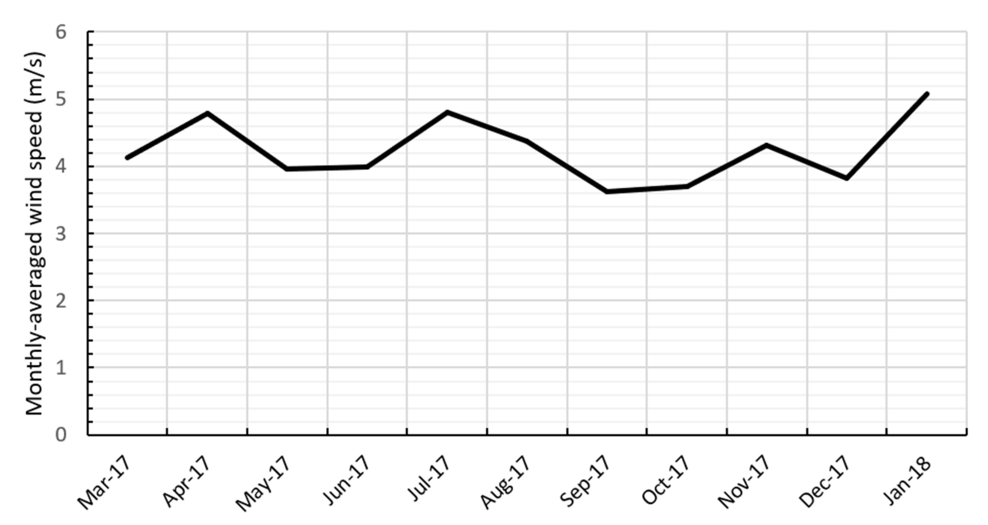
Figure 10 illustrates the monthly average wind speeds at the NERC site, as drawn from the collected data. Additionally,

Table 3. Frequency distribution of wind speed.

Wind Speed Class (m/s)	Average Wind Speed (m/s)	Frequency	Frequency Percentage	Cumulative Frequency Percentage
0.01–1.00	0.749	540	1.20%	1.20%
1.01–2.00	1.603	4010	8.70%	9.90%
2.01–3.00	2.530	8309	18.10%	28.00%
3.01–4.00	3.491	9986	21.70%	49.70%
4.01–5.00	4.482	8460	18.40%	68.10%
5.01–6.00	5.472	6621	14.50%	82.60%
6.01–7.00	6.454	4328	9.40%	92.00%
7.01–8.00	7.436	2222	4.80%	96.80%
8.01–9.00	8.419	889	2.00%	98.80%
9.01–10.00	9.429	386	0.80%	99.60%
10.01–11.00	10.413	115	0.20%	99.80%
11.01–12.00	11.442	38	0.10%	99.90%
12.01–13.00	12.484	19	0.10%	100.00%
13.01–14.00	13.416	10	0.00%	100.00%
14.01–15.00	14.942	1	0.00%	100.00%
15.01–16.00	15.638	2	0.00%	100.00%

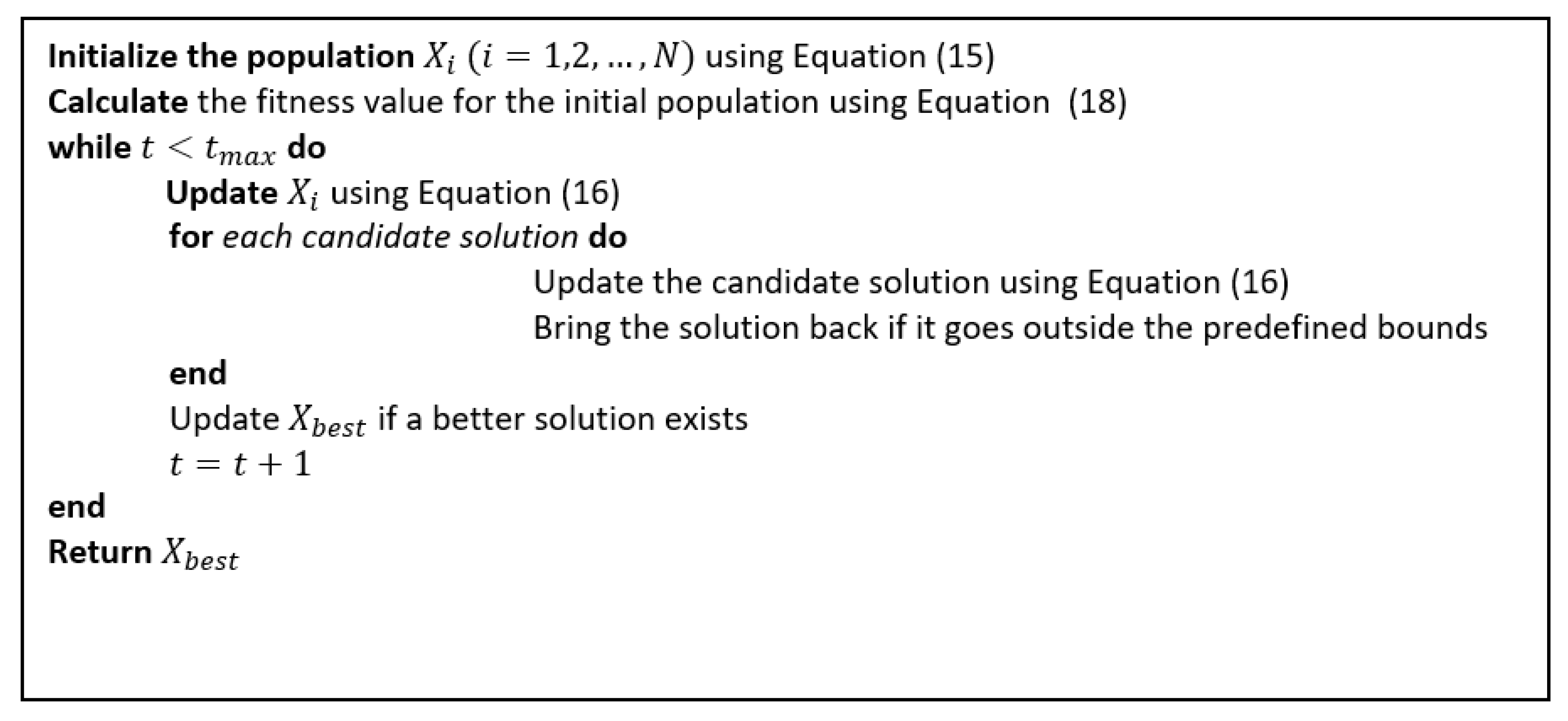
lists the average wind speed, frequency, frequency percentage, and cumulative frequency percentage corresponding to equal-width wind speed classes. Table 2 provides the parameters specific to the FA technique, among them the stopping criterion, which was 1000 iterations, that we used to obtain high-accuracy results. It took the FA algorithm less than 200 iterations to reach the steady state, meaning that the fitness value converges or an exact solution is reached. Figure 11 shows that the convergence to the optimal solution occurred approximately after 100 iterations. It is worth mentioning that the researchers in this study relied on Python code to execute the artificial intelligence algorithm.

Following the statistical analysis and the parameter estimation methods described above,

Table 4. Analysis summary.

Method	$\mathit{k}$	$\mathit{c}$	Average Wind Speed	RMSEPP	RMSEQQ	R2PP	R2QQ	MAEPP	MAEQQ	KS
EPFM	1.918	9.174	8.14	0.3176	0.0672	0.117	0.2109	0.2674	0.0559	0.5208
FA	2.197	4.211	3.73	0.0056	0.0229	0.999	0.908	0.0033	0.014	0.0139
GM	2.043	4.967	4.4	0.0631	0.0198	0.965	0.9316	0.0423	0.0142	0.1255
LSM	1.213	6.869	6.44	0.1898	0.055	0.685	0.471	0.1643	0.0445	0.3157
MOM	2.469	4.778	4.24	0.0529	0.0092	0.975	0.985	0.0315	0.0061	0.1278

delivers the shape and scale estimates associated with every technique. Consequently, it is clear from the demonstrated results that the FA has the best prediction potential regarding every testing metric used, followed by the MOM and GM. For example, using the FA method, the K–S number corresponding to the extracted shape and scale parameters is the most accurate as it tends to zero. 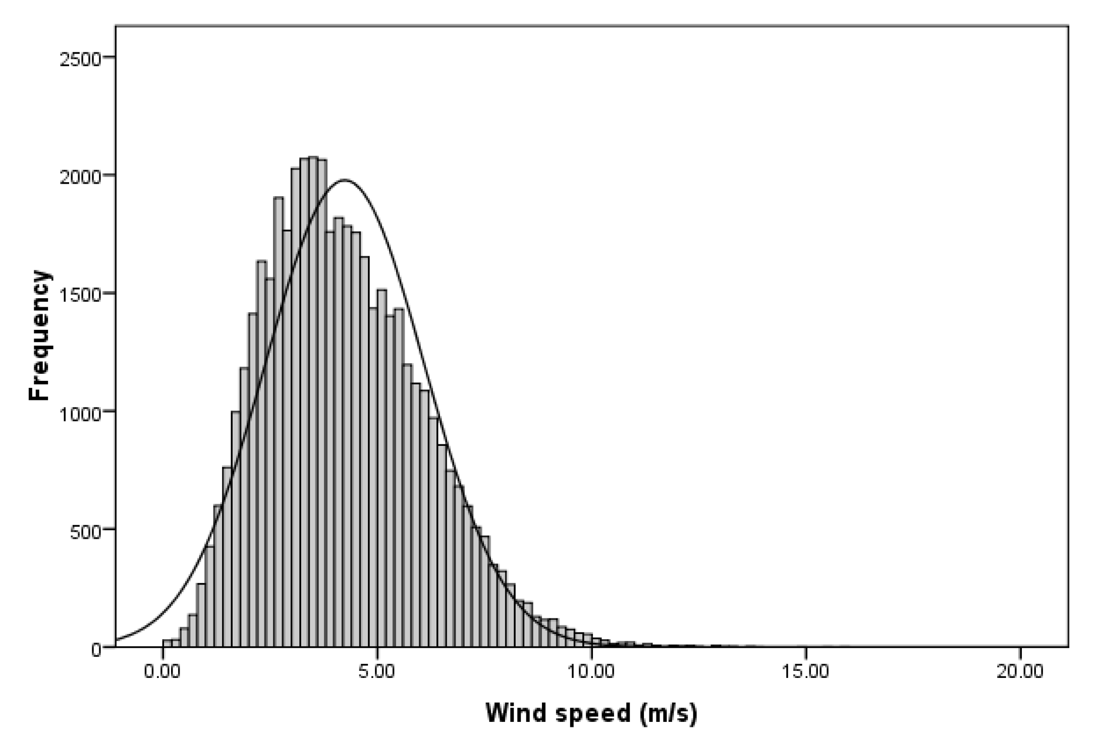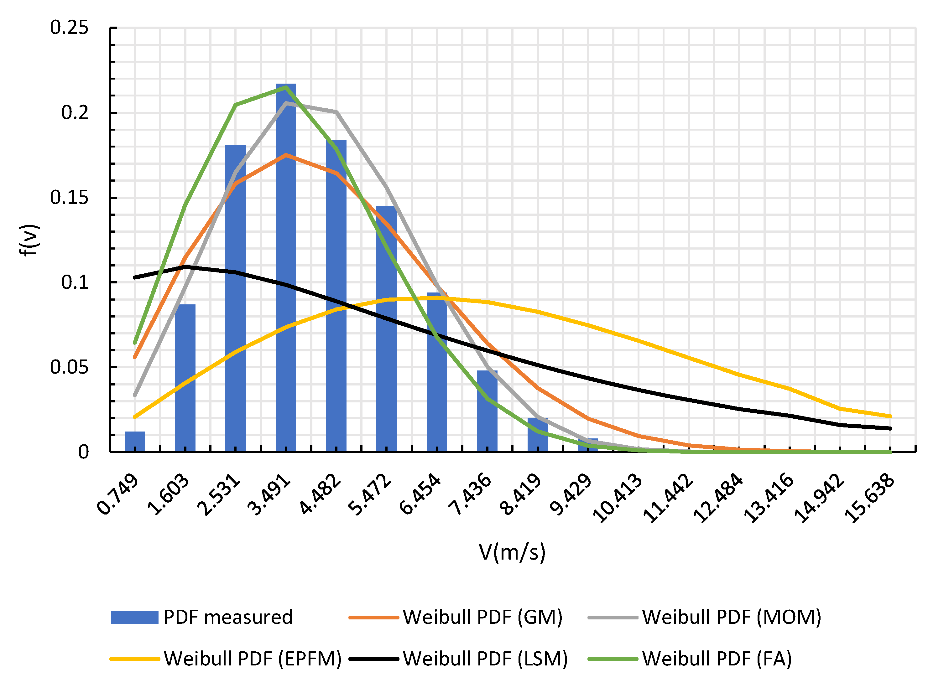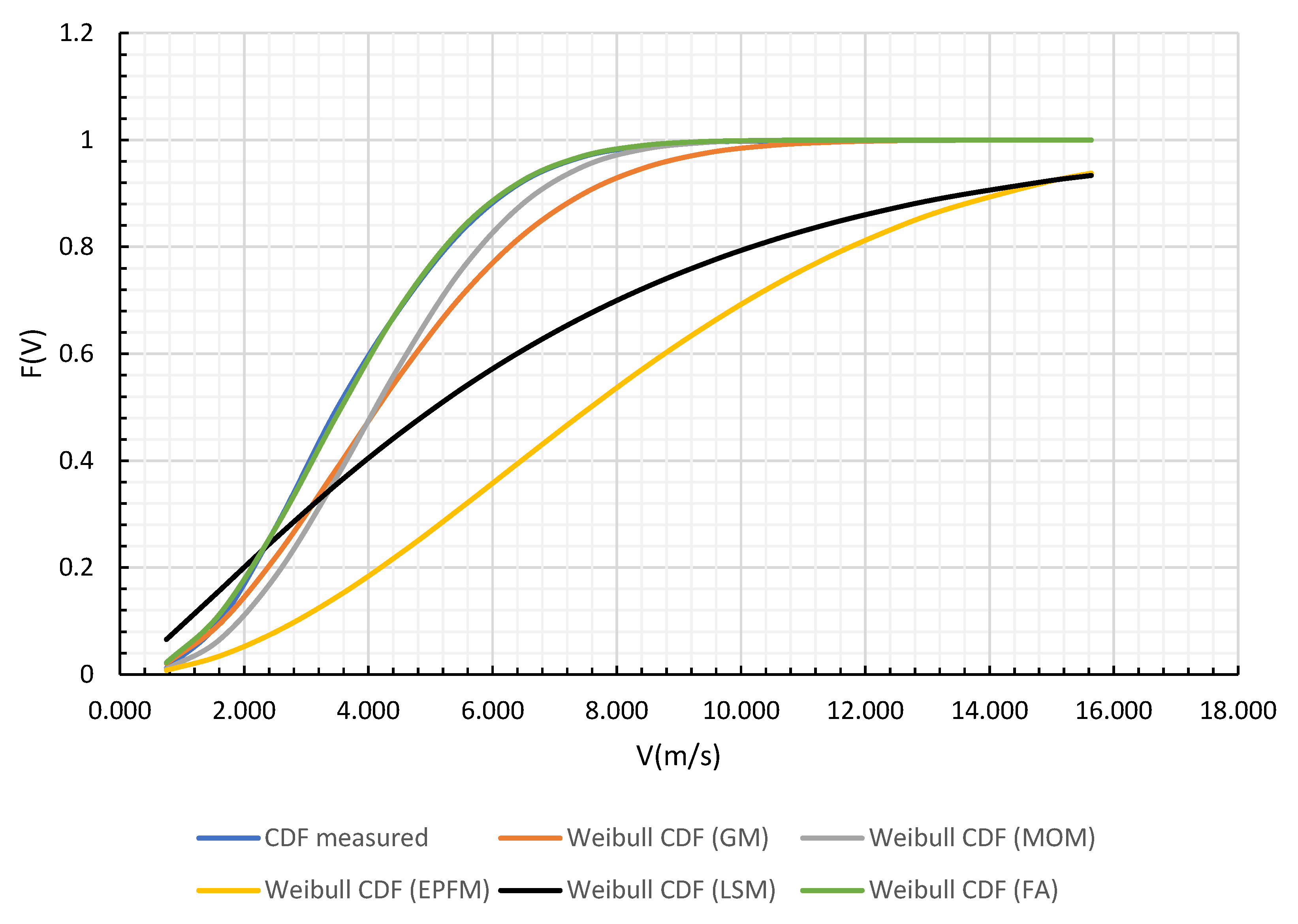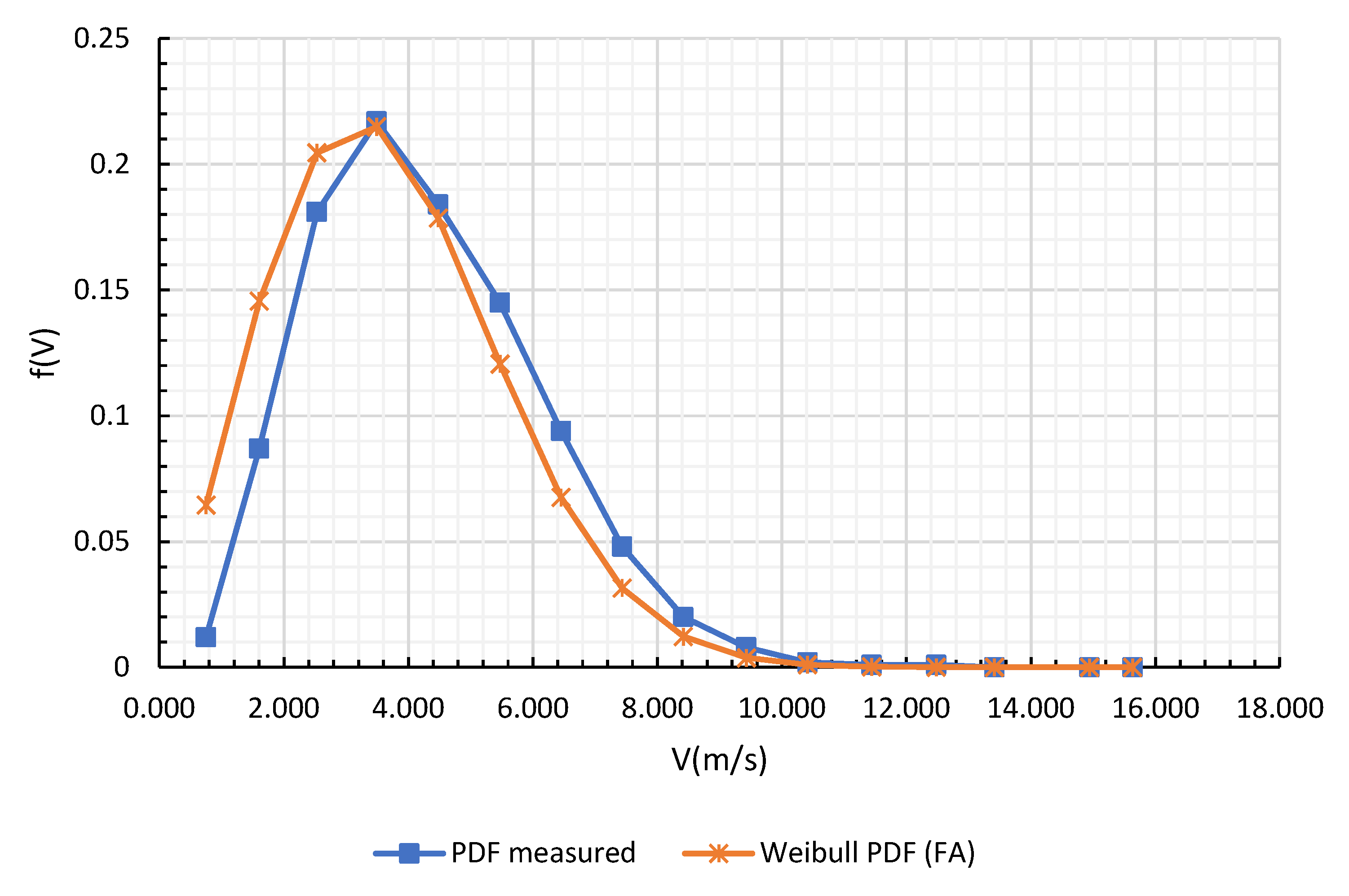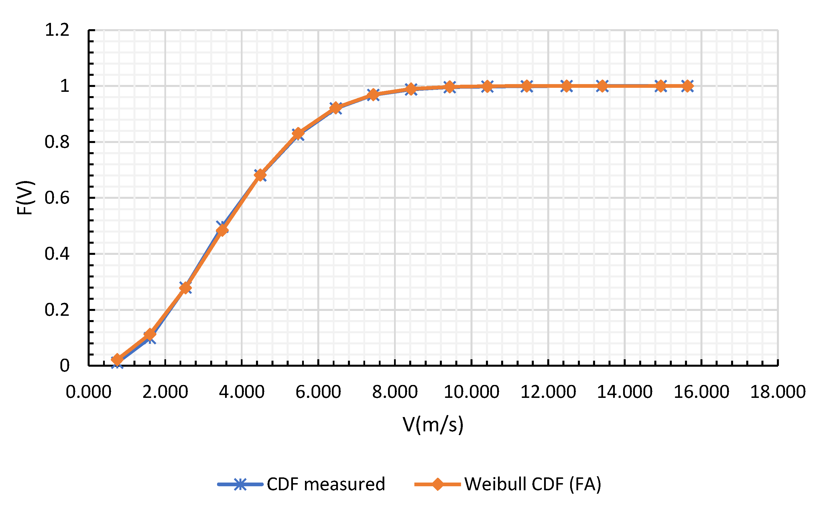The LSM and EPFM showed a weak performance looking at the R²_PP and R²_QQ. If we rely on visual comparison and inspection to determine the quality of the methods used in estimating the parameters of the Weibull distribution, then Figure 12, Figure 13, Figure 14 and Figure 15 explicitly show the superiority of the artificial intelligence technique. Additionally, these figures prove that the Weibull distribution perfectly describes the wind data at the NERC site. We can understand the dominance of the FA over the rest of the prediction methods due to the apparent nonlinearity in the wind speed data by looking at the regression analysis results in

Table 5. Regression analysis result of the wind speed data.

Statistic	Value
R	0.003
R2	0.000
Adjusted R2	0.000
Standard Error	1.85
Significance F (ANOVA test)	0.538

, which favors the stochastic metaheuristic methods in such cases. Moreover, the average wind speeds were evaluated by employing $\widehat{k}$ and $\widehat{c}$ to Equation (3), and are given in Table 4. The average speed corresponding to the FA method equals $3.73 \mathrm{m}/\mathrm{s}$.

The average speed for the wind energy assessment must also consider the dataset’s power content. Hence, the weighted average expression represented by Equation (23) was used [43], and a $4.98 \mathrm{m}/\mathrm{s}$ was obtained.

It is worth mentioning that although the FA method has a high prediction accuracy, the average wind speed produced by the classic techniques (i.e., MOM and GM) are closer in magnitude to the weighted average speed. Even after the visual inspection of the wind speed data given in Figure 10, it is noticeable that the classically produced numbers rest within the region of most data points. On the other hand, looking at the frequency percentages delivered in Table 2, the wind speed class that embraces the average speed produced by the FA method has the highest frequency, making the FA values more realistic in forecasting.

$$V_m={\left(\frac{1}{n}{\displaystyle \sum }_{i=1}^n{V}_i^3\right)}^{1/3}$$

(23)

where $V_m$ is the average wind speed, $n$ is the sample size, and $V_i$ are the observations or wind speeds.

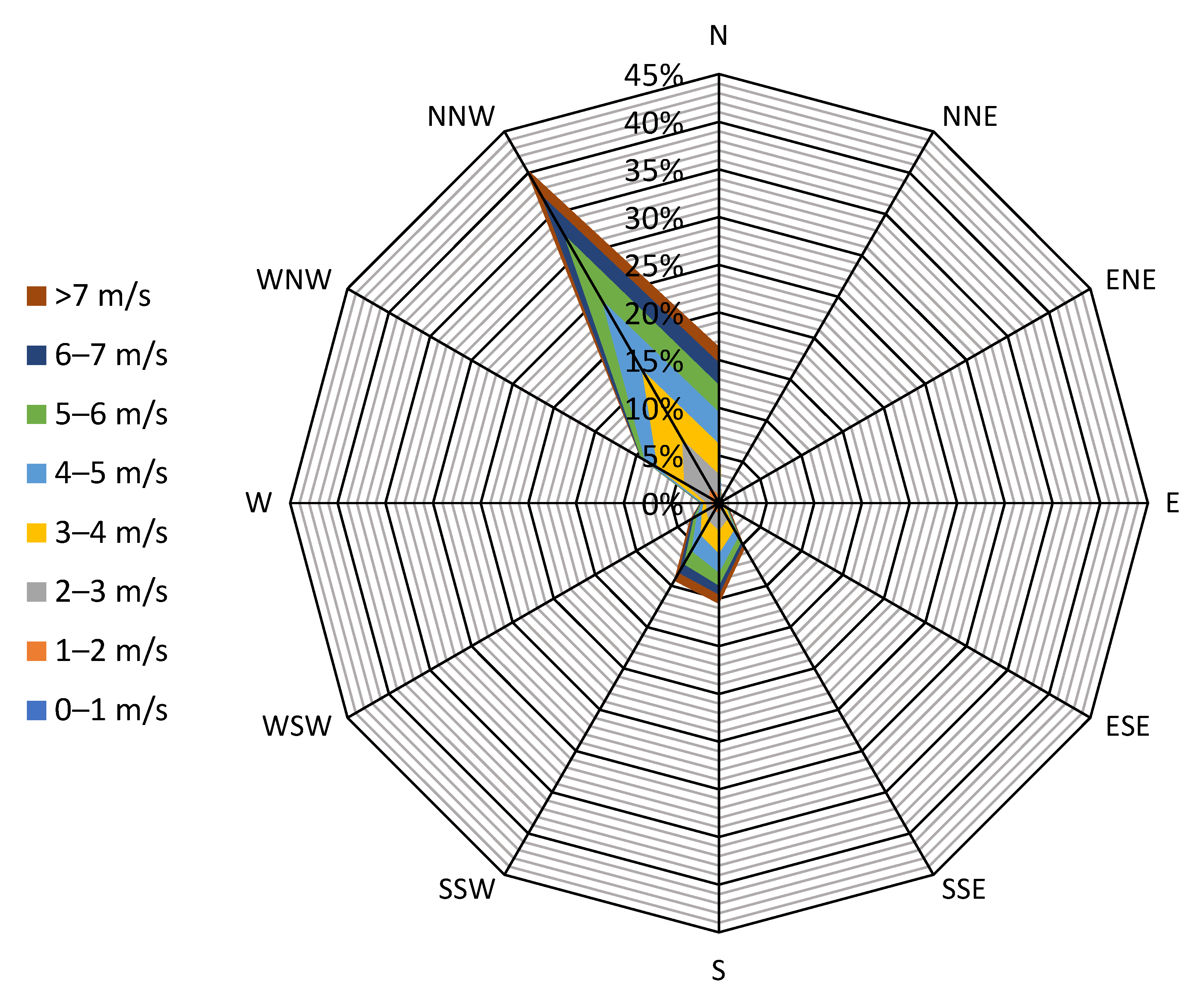
Finally, the frequency percentage data in

Table 6. Frequency distribution of wind speed per wind direction.

Wind Direction (Degree)	Wind Direction	Average Wind Speed	Frequency Percentage
345–15	N	4.2384	16.029%
15–45	NNE	3.9889	4.075%
45–75	ENE	2.88	1.398%
75–105	E	3.23	1.431%
105–135	ESE	4.066	2.494%
135–165	SSE	3.997	8.411%
165–195	S	4.285	13.903%
195–225	SSW	4.51	10.669%
225–255	WSW	3.686	3.500%
255–285	W	2.763	1.727%
285–315	WNW	3.213	7.339%
315–345	NNW	4.567	29.046%
Total			100%

, which corresponds to the wind direction, indicates that the wind primarily blows from the north, which is again noticeable in the rose diagram in Figure 16. The wind direction illustrated in the rose diagram precisely simulates reality according to our on-field remarks that we have noticed monitoring our currently operating 2 kW_p wind turbine recently installed at the NERC campus.

5. Conclusions

In this research, we presented the results of the statistical analysis performed on wind speed and direction data collected by a weather mast station installed at the NERC, Soba, Khartoum. Limited data filtering was applied to detect and remove error codes, and then filling in the gaps was performed using the simple arithmetic mean of the remaining data points, as the distorted data fields were considered trivial (i.e., $n=20$) compared to the whole dataset (i.e., $n=45,936$) in terms of size. Firstly, we obtained the Weibull distribution parameters using analytical and stochastic methods, shown in Table 4. In this table, the FA method outperforms the others in the goodness-of-fit. The MOM and the GM rank second and third, while the EPFM performs weakest. The best value for the shape parameter is 2.197, while the worst value is 1.918. The best value for the scale parameter is 4.211, while the worst value is 9.174. Secondly, the nonlinearity in wind speed data, which was conveyed in the regression analysis results provided in Table 5, explains the advantage of the FA method over the conventional ones, as the artificial intelligence methods best fit nonlinear data. Thirdly, the rose diagram shows wind mainly blowing from the north, which complies with the real-world scenario. Finally, the average wind speed, according to the FA results, is equal to $3.73 \mathrm{m}/\mathrm{s}$, while the weighted average speed equals $4.98 \mathrm{m}/\mathrm{s}$. Still, the weighted average value looks more realistic from the field measurements point of view, but the FA average figure better serves the forecasting purpose due to the high accuracy applied while obtaining this number coupled with the high frequency of occurrence of this speed. The novelty in this work is reflected in the use of data generated in Sudan to forecast local wind speeds using the FA technique, which is widely used in solar PV modeling. Additionally, since classic estimating approaches execute differently location-wise, assessing their efficacy becomes new, which was achieved here. The authors can present several recommendations regarding the assessment of the local wind energy resource and the optimal use of this potential based on the cutting-edge technologies available in the global market:

• A higher and multi-anemometer mast wind station must be installed locally to facilitate the vertical extrapolation of wind speed in heights compatible with utility-scale power production.
• Figure 15 demonstrates the high capacity of stochastic methods, in particular the swarm intelligence algorithms, in predicting the wind speed in the region, making this technique the best choice for domestic meteorological and forecasting research.
• Private sector participation in power generation from clean energy resources such as wind can fill the energy demand gap in Sudan. Hence, soft financing means provided by the stakeholders and international institutions will be the base for such contributions.
• Wind turbine manufacturers need to deploy pilot projects in the country, preferably under the supervision of the NERC, to inspect the prospects of this investment.