Article

Filling Missing and Extending Significant Wave Height Measurements Using Neural Networks and an Integrated Surface Database

Faculty of Civil Engineering, University of Zagreb, 10000 Zagreb, Croatia
*
Author to whom correspondence should be addressed.
Wind 2023, 3(2), 151-169; https://doi.org/10.3390/wind3020010
Submission received: 17 February 2023 / Revised: 17 March 2023 / Accepted: 21 March 2023 / Published: 28 March 2023
(This article belongs to the Special Issue Advances in Solid and Fluid Mechanics for Offshore Wind Turbines)

Abstract

:
Wave data play a critical role in offshore structure design and coastal vulnerability studies. For various reasons, such as equipment malfunctions, wave data are often incomplete. Despite the interest in completing the data, few studies have considered constructing a machine learning model with publicly available wind measurements as input, while wind data from reanalysis models are commonly used. In this work, ANNs are constructed and tested to fill in missing wave data and extend the original wave measurements in a basin with limited fetch where wind waves dominate. Input features for the ANN are obtained from the publicly available Integrated Surface Database (ISD) maintained by NOAA. The accuracy of the ANNs is also compared to a state-of-the-art reanalysis wave model, MEDSEA, maintained at Copernicus Marine Service. The results of this study show that ANNs can accurately fill in missing wave data and also extend beyond the measurement period, using the wind velocity magnitude and wind direction from nearby weather stations. The MEDSEA reanalysis data showed greater scatter compared to the reconstructed significant wave heights from ANN. Specifically, MEDSEA showed a 22% higher HH index for expanding wave data and a 33% higher HH index for filling in missing wave data points.

1. Introduction

Knowledge of significant wave heights at a site is important for the management of maritime activities [1], the design of floating offshore wind turbines (FOWT) [2], the design of flood protection measures [3], and coastal vulnerability assessments [4]. For example, wind energy, which is a clean and efficient renewable energy source [5], could be harvested with FOWTs [6]. However, FOWTs are exposed to forces such as sea waves and sea currents that can reduce production and lead to faster fatigue of the exposed marine turbines [7,8]. Therefore, accurate and reliable long-term wave data are of paramount importance to marine and coastal engineers for structure design [9].
Unfortunately, important long time series of wave measurements are often plagued with missing data or simply extended periods without conducted measurement campaigns [10]. Wave buoys providing wave climate measurements could be continuously maintained by various national or international climate monitoring networks (e.g., Spanish Harbor Authority [11]) or sporadic wave measurements during certain measurement campaigns [12].
Several methods are available to fill in missing data or extend wave measurement data, such as simplified empirical models [12,13] or complex local numerical wave models [14,15], as well as climate wave reanalysis products [16] or the combination of local numerical models with regional or global wave reanalysis products through the downscaling procedure [17,18,19]. Nevertheless, regional or global numerical models are limited by available computing power, detailed bathymetry data, their complexity, and difficult-to-determine coefficients (e.g., white-capping parameters, bottom frictional dissipation, depth-limited wave breaking, etc.) [20], while the main advantage is that they perform physically based calculations. To avoid computer resource challenges, reanalysis products often have relatively large numerical cells, but include a complete record of changes in weather and climate over decades. The size of numerical cells for reanalysis products is typically 0.5° × 0.5° [21] and 0.25° × 0.25° [22] for global reanalysis products, or even 1/24° × 1/24° for regional reanalysis products [23], with a temporal resolution between 1 h and 3 h. This resolution is not detailed enough for the wind forcing or wave model itself to accurately represent shallow, enclosed areas bounded by complex topography [23]. For example, the MEDSEA reanalysis model [23] is the most detailed Copernicus numerical model reanalysis for the Mediterranean Sea (in both spatial and temporal terms). In reporting the accuracy of the MEDSEA reanalysis product, Korres, Ravdas [23] still observed low accuracy when validating the reanalysis data with buoy measurements in well sheltered areas, such as the Adriatic Sea.
Although not constrained by physical laws, machine learning methods are proving to be a computationally efficient way to fill in missing wave data. Machine learning models are capable of mapping complex nonlinear functions between inputs and outputs when sufficient training data are available [24]. It should be noted that these techniques are used in many areas of marine and coastal engineering, such as wave forecasting with a lead time of several hours [1,20,25,26,27], wave hindcasting from a regional to a local scale [11,28], wave runup [29], beach sediment transport [30,31], beach nourishment requirements [32], etc. In addition, machine learning models have been used when data are missing in the measured wave time series to fill in the missing wave heights [33,34] or to find a mapping function between multiple nearby wave buoys at nearshore locations [35]. Features used in the input layer are typically offshore wind measurements at the wave buoy itself [6], wave measurements of other nearby wave buoys [33,35], or reanalysis sourced model data [11,20,34,36]. The accuracy and feasibility of machine learning techniques are highly dependent on the quality and source of input features. Easily accessible input feature data could promote future use [37].
This study aims to propose a machine learning method, specifically artificial neural networks (ANNs), that uses publicly available onshore meteorological measurements from nearby weather stations for filling and extending significant wave heights in a sheltered and complex topographic case. The meteorological measurements are from NOAA’s publicly available Integrated Surface Database (ISD) [38,39,40]. The feasibility of the ANNs is tested using state-of-the-art regional reanalysis wave data (MEDSEA), which covers the entire Mediterranean Sea and is maintained at the Copernicus Marine Service. The study area is in the Adriatic Sea, which has proven to be the most challenging region for MEDSEA. In addition, we are testing the capability of the ANN to extend the wave time series beyond the duration of the buoy measurement campaign. It should be noted that the proposed method of filling in missing wave measurements at sheltered locations is not as computationally expensive compared to numerical wave modeling when using an established machine learning model.
This article is organized as follows: Section 2 explains the methodology, Section 3.1 examines the significance of each feature using a univariate feature ranking, Section 3.2 compares machine learning-filled wave data with measured data, and Section 3.3 analyzes the potential for extending the wave measurements. Section 4 and Section 5 provide the discussion and conclusions of the paper.

2. Materials and Methods
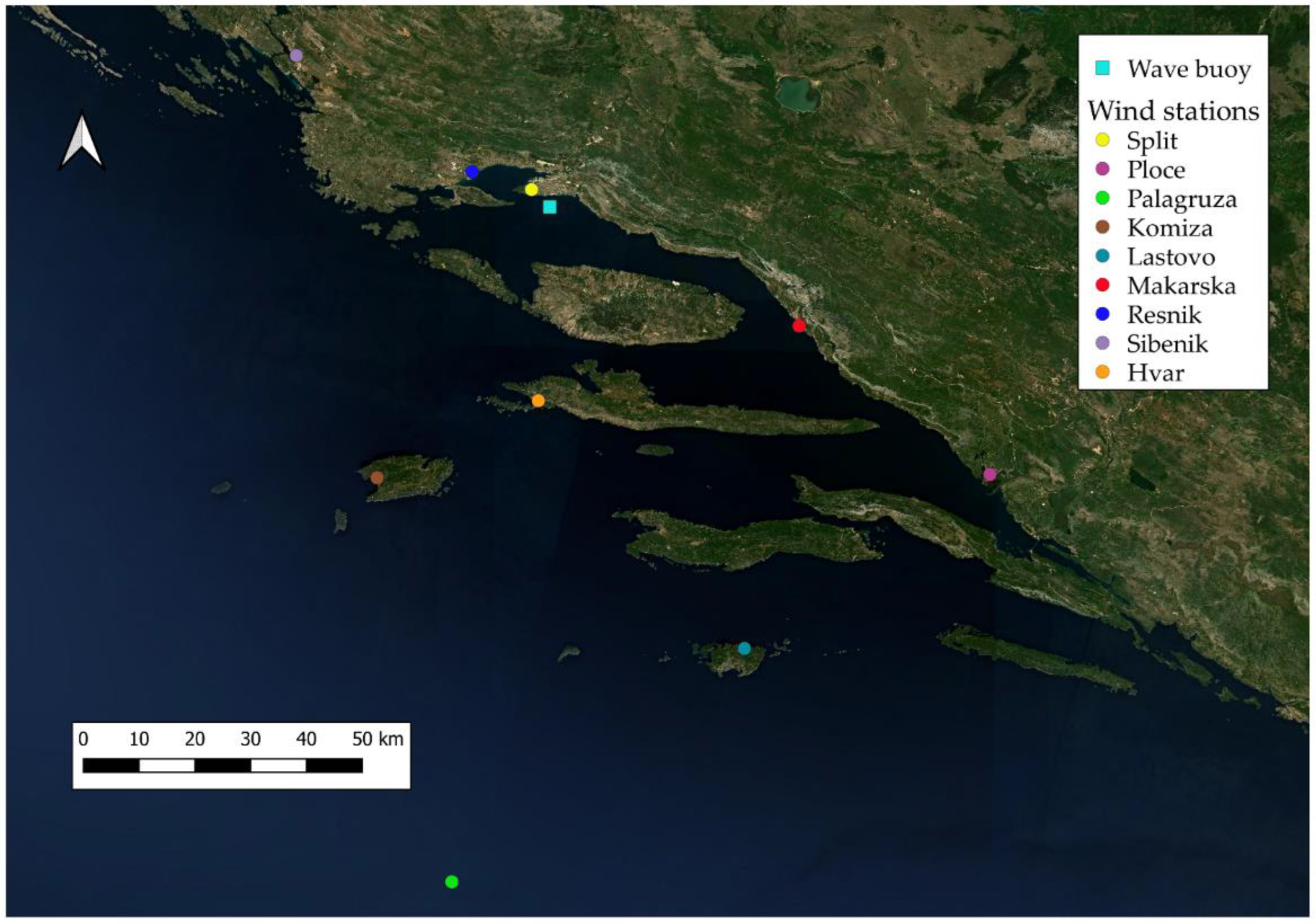
2.1. Study Site

The research area includes the area around Split, Croatia, on the mid-latitude Adriatic Sea, as shown in Figure 1. The area is complex, with two islands in the southwest (Šolta and Vis) and four islands in the southeast (Brač, Hvar, Korčula and Lastovo). The wave buoy measurements were collected off the port of Split (43.48833° N, 16.46500° E) (shown with cyan rectangle in Figure 1). Wind-driven waves dominate on the location of Split, as the surrounding islands protect the site from offshore swells. Therefore, the local winds (mainly bora (NE) and scirocco (SE)) dictate the significant wave heights observed at the wave buoy off Split. This leads to the hypothesis that weather data from surrounding weather stations, which include the wind velocity magnitudes and wind direction, could have significant explanatory power to fill in missing data or extend the wave data.

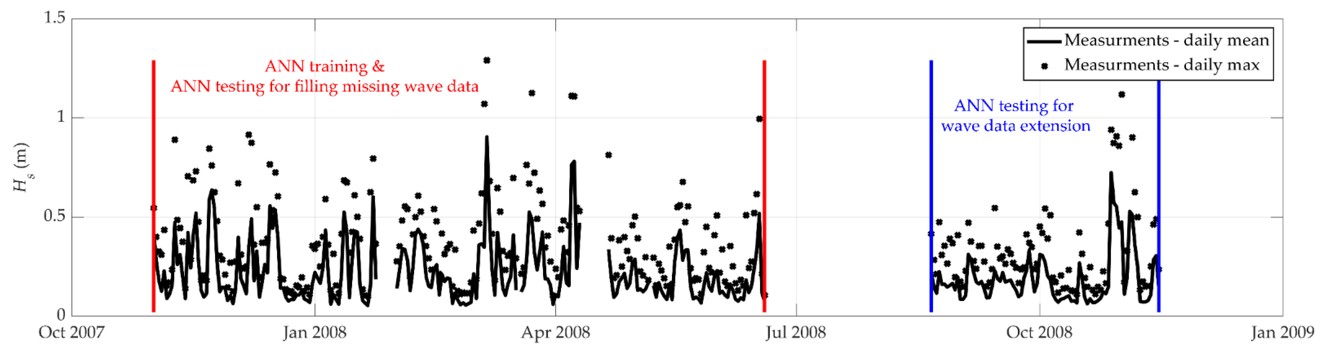
2.2. Wind and Wave Data

Wave measurements were made using the well-known DATAWELL Waverider DWR MKIII anchored in cooperation with the Hydrographic Institute of the Republic of Croatia. The GPS-tracked and anchored Waverider measures wave direction, wave height and peak period. Figure 2 shows a time series of significant wave heights during the wave buoy measurement period from November 2007 to November 2008, with a measurement gap in summer. The wave time series shows a typical year in terms of wave climate. The hourly significant wave height reached 1.29 m on 6 March 2008, the most extreme value for this fetch-limited location (Figure 2). During the measurement period of the buoy site, the average wave height was very low, at 0.21 m (Figure 2). The significant wave heights measured were predominantly in the range of 0.1 m–0.2 m. Figure 2 shows the training period (1 November 2007 to 19 June 2008) for the ANN training and fill testing with missing wave data (separated by red vertical lines). Blue vertical lines separate another test period for testing the trained ANN for wave measurement extension (8 August 2008 to 15 November 2008). Both periods show prominent energetic events for the region under study, making them suitable for ANN training and testing.
The ANN method can generally be used to hindcast the significant wave height given in this study, as well as other wave parameters such as wave period or wave direction. However, we did not consider the wave period in this paper because we did not have enough data (only 2 months of wave period measurements for the considered Split site, from September 2008 to October 2008; see Figure 2).
Weather observation data from the Integrated Surface Database (ISD) were used as features in the input layer of the ANN. The ISD is a global database of synoptic observations compiled from numerous sources and archived and maintained at NOAA [38,39,40]. The ISD contains many parameters at hourly intervals, including wind velocity and direction, temperature, dew point, sea level pressure, etc. In this paper, we extracted the weather data available in the ISD from weather stations near the location of the wave buoy.
Unfortunately, there are missing data in the weather data obtained from ISD. These data points are subjected to exploratory data analysis and data cleaning. As a result of the initial visual analysis, it was determined that some parameters simply do not have data for the station and time period in question, such as wind gusts, precipitation, etc. These empty variables are considered useless, and can therefore be discarded. The variables that provided some data for the weather stations are listed in Table 1 (the locations of the weather stations are shown in Figure 1). A complete list of weather stations with geographic details can be found in Table 2.
The 6 hourly parameters that provide data are still plagued by missing data. If all ‘NaN’ (Not A Number) data points were discarded, too few data points would remain for ANN training and testing. Therefore, missing data gaps that were less than 5 h long were filled in by linear interpolation between the bounding known data points for each variable. If the data gap was longer than 5 h, the data points were simply excluded from further consideration.
To benchmark the accuracy of the ANN, we used a 27 year wave reanalysis for the Mediterranean Sea, MEDSEA [23] (maintained and distributed by Copernicus Marine Service). This wave reanalysis is based on the advanced third generation wave model WAM Cycle 4.6.2 [14,41]. It explicitly solves the wave transport equations without taking the form of the wave spectrum. The included source terms were wind input, white-capping dissipation, nonlinear transmission, and bottom friction. The wind and white-capping dissipation terms were based on Janssen’s quasilinear theory of wind wave generation [42,43], while the empirical JONSWAP formulation was used for the bottom friction term [44]. The numerical model discretized the wave spectra, with 32 frequencies covering a logarithmically scaled frequency band from 0.04177 Hz to 0.8018 Hz and 24 uniformly distributed directional bins (bin size of 15 degrees). Winds from the ERA5 reanalysis 10 m above the sea surface (Copernicus Climate Service—ECMWF) forced the numerical wave model. The bathymetric map was created using the GEBCO bathymetric dataset [45]. The MEDSEA reanalysis model provided hourly 2D instantaneous fields (Table 2) with a horizontal resolution of 1/24°.
Importantly, the MEDSEA reanalysis incorporates a data assimilation procedure that uses significant wave heights obtained from altimeters and adjusts the resulting wave spectrum at each grid point accordingly (originally developed by [46]). This method allows the reanalysis to achieve higher accuracy compared to the initial ‘first guess’ outputs of the WAM numerical wave model.

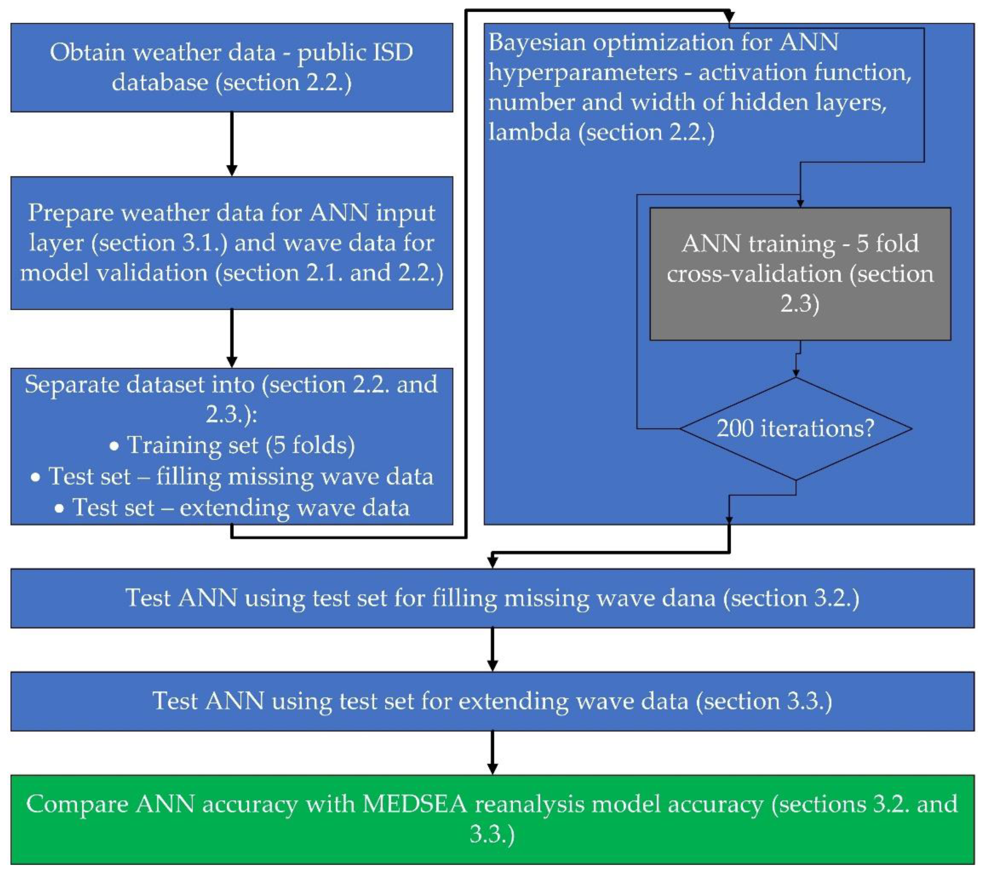
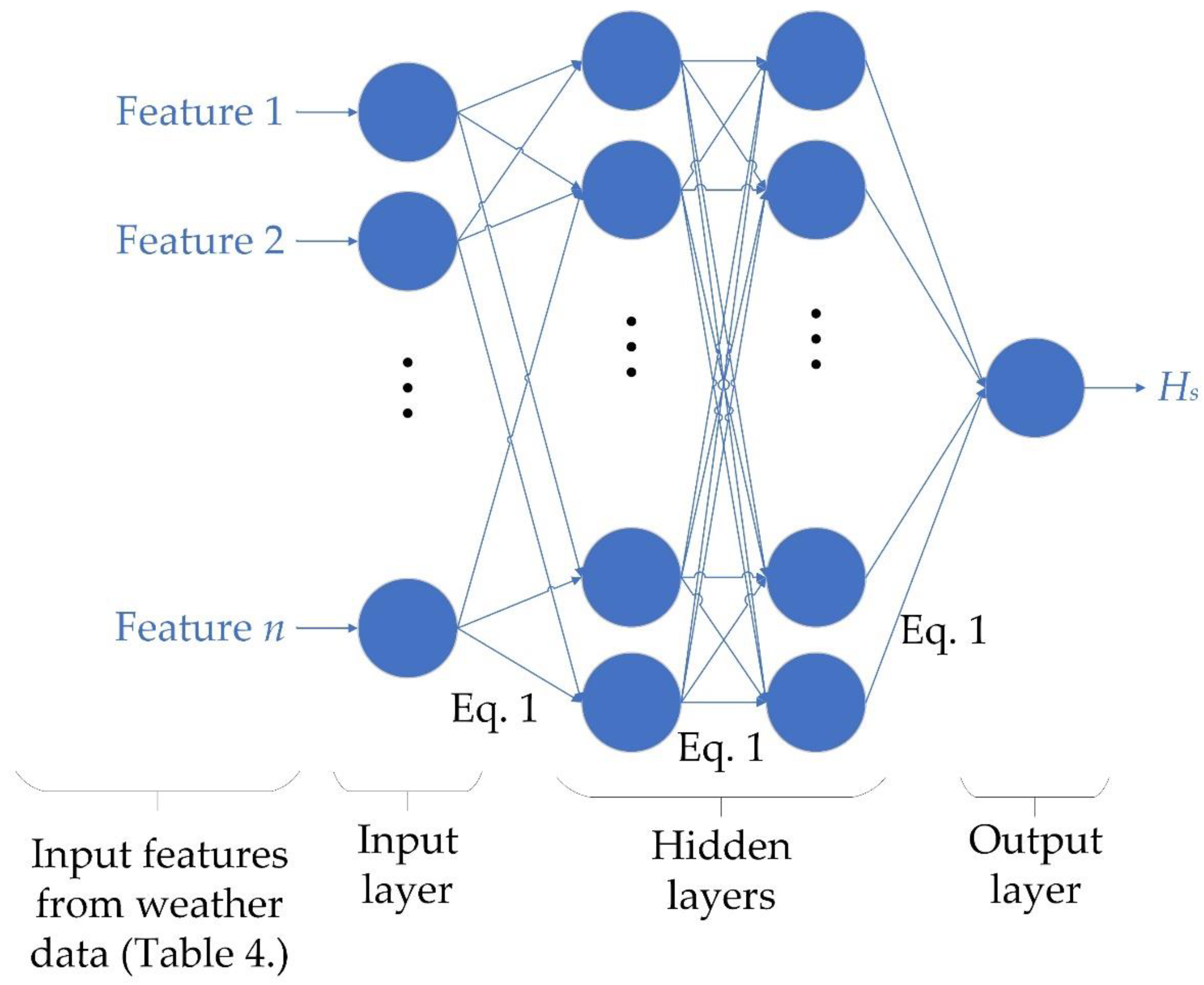
2.3. Artificial Neural Network Training and Model Building Workflow

The ANN building workflow that was used in the paper is summarized in Figure 3, with corresponding sections for a detailed explanation of the various steps undertaken during the ANN model building and accuracy testing.
Prior to the training procedure, we randomly flagged 20% of the data points from the wave time series from 1 November 2007 to 19 June 2008 as “missing” data points (separated by red vertical lines in Figure 2). These data points were discarded from the training dataset to avoid data leakage. The remaining 80% of the time series were used for ANN training. The discarded 20% of data points marked as ‘missing’ were used to test the ability of ANN to fill in random missing data points in the data (results are shown in Section 3.3). The wave time series from 8 August 2008 to 15 November 2008 (separated by blue vertical lines in Figure 2) was used exclusively to test the ability of ANNs to extend the wave time series to a period outside the training period (results shown in Section 3.4). The input and response data were preprocessed to improve the efficiency of the ANN training procedure. Preprocessing included normalizing the inputs and outputs to fall within the range [–1,1] to avoid the vanishing gradient phenomenon. The question of which weather data features should be fed into the ANN was examined using univariate feature ranking (results shown in Section 3.1).
The ANN model itself (gray rectangle in Figure 3) is a regular multilayer feed-forward network, which is commonly used to fit non-linear functions that relate the input data (wind data from ISD, as described in Section 2.2) to the response data (measured wave data, as described in Section 2.2) [24]. Each node (blue circle in Figure 4) passes information, starting from the input layer to the next layer until the output layer [47]. An ANN usually consists of nodes arranged in an input, multiple hidden layers, and an output layer (Figure 4). In this paper, the output layer consists of only one node corresponding to the significant wave height.
Information is passed from the input nodes through the nodes in the hidden layers up to the output layer using the following formulation (arrows in Figure 4):
h j = f a j + i = 1 n w i x i
where xi are the input features, hj are the responses of the subsequent node, wi are the weights, aj are the biases, and f is the activation function.
The ANN training process determines the weights and biases in Equation (1) that connect each node to the nodes in the subsequent layers using the backpropagation algorithm. The algorithm minimizes the difference between the ANN significant wave height prediction and measurements.. The algorithm used the memory-constrained Broyden–Fletcher–Goldfarb–Shanno quasi-Newton algorithm (LBFGS), where the mean square error (MSE) is the optimization objective for training the weights and biases [48]. The usual 5-fold cross-validation was performed during training on the training set to minimize overfitting of the ANN weights and biases to the training data. This paragraph about ANN training is related to one iteration in the Bayesian optimization process, as shown in Figure 3.
To automate the process to some extent, Bayesian optimization (Figure 3) was used to find the best possible values for the hyperparameters for ANN training, such as the activation function, the lambda value for model regularization, and the number and width of the hidden layers. The Bayesian optimization process trained the ANN’s weights and biases 200 times with varying hyperparameters in order to find the best hyperparameter combination for ANN construction and training. The Bayesian optimization process chose the smallest mean square error (MSE) to determine the best possible hyperparameter combination.

2.4. Statistical Error Metrics

The filling and extending capabilities of the trained ANN and the MEDSEA reanalysis model were examined using the statistical errors metrics. These include the scatter indices such as HH proposed by Hanna and Heinold [49] and the normalized root mean square error (NRMSE), and also the common Pearson correlation coefficient (R), along with the normalized bias (NBIAS). These are described in Equations (2)–(5):
R = i = 1 N P i P ¯ O i O ¯ i = 1 N P i P ¯ 2 i = 1 N O i O ¯ 2 1 / 2
H H = i = 1 N P i O i 2 i = 1 N P i O i
N B I A S   = P ¯ O ¯ O ¯
N R M S E = i = 1 N P i O i 2 i = 1 N O i 2
where N is the number of data points examined, Pi and Oi denote the model prediction and observation, respectively, while the overbar indicates respective mean values.
NRSME has shown unrealistically good accuracy toward predictions, with negative bias in previous research, so the HH index is generally recommended for quantifying scattering errors [50]. A high value indicates high scatter, and therefore high error for both HH and NRMSE indices, and thus a smaller value is preferred.

3. Results

To determine which features of the input dataset are most valuable in constructing an ANN, a univariate feature ranking is presented in Section 3.1. Depending on the amount of input data used in the input layer of ANN, three different machine learning models are created. Next, the machine learning models are trained in Section 3.2 and tested for filling missing wave data from the wave buoy in Section 3.3. Finally, the same machine learning models are tested for accuracy in expanding the wave time series outside of the original training and testing period in Section 3.4. These machine learnings are also benchmarked against the MEDSEA reanalysis filling and extension capabilities.

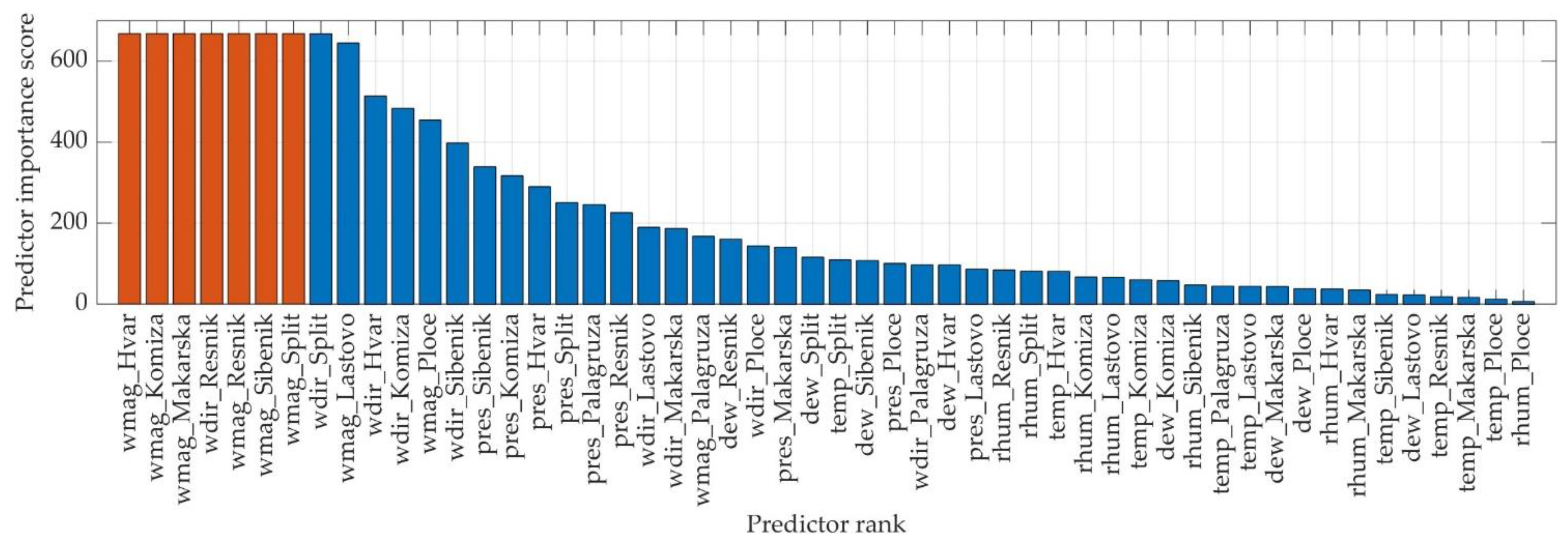
3.1. Univariate Feature Ranking

Feature selection consists of determining a subset of input features from all existing features that show a high explanatory power. In this paper, the F-test was conducted to perform the feature selection. If the F-test results in a small p-value, then the feature is significant. Subsequently, all predictors in the ISD dataset were ranked according to their significance (Figure 5), with the results presented as the negative logarithm of the p-value (−log(p)). When a p-value is close to zero, the output would be Inf. Therefore, the features that had an Inf score were colored orange instead of blue and scaled to the largest non-Inf score that was blue. Overall, a higher score value in Figure 5 means that the corresponding predictor is more important.
The highest ranked features all related to wind at different weather stations (wind velocity magnitude and wind direction). In particular, the wind velocity magnitudes at the weather stations of Hvar, Komiza, Makarska, Split, Resnik and Sibenik are all included in the top 7, as is the wind direction at Resnik. The wind velocity magnitude features that performed less well were measured at the Ploce, Lastovo and Palagruza weather stations. This seems reasonable since these stations are farthest from the location of the wave buoy (wave buoy and wind station locations shown in Figure 1).
Some weather stations were discarded even though they had high scores because the number of available data points was still low (Table 3), even after the data cleaning described in Section 2.2. Stations with available data points below the 95% threshold were Lastovo, Makarska, Palagruza, and Ploce (Table 3). A small number of data points of input features would greatly reduce the number of wave height reconstructions possible with a trained ANN, and is therefore undesirable. Overall, this resulted in the removal of features such as wmag_Makarska that had high predictor importance due to a small number of data points.
In total, three different ANN models were created with a different number of input features in the input layer. These three ANN models contained the first available 6, 8, and 10 ranking features (Table 4). The other features were discarded as unimportant for further analysis.
A matrix of Pearson correlation coefficients between input features was created to avoid including redundant information in the ANN (not shown here for brevity). Features such as air temperature, dew point temperature, and barometric pressure were frequently correlated with each other at different weather stations, but are still not included in the 10 highest ranked variables.

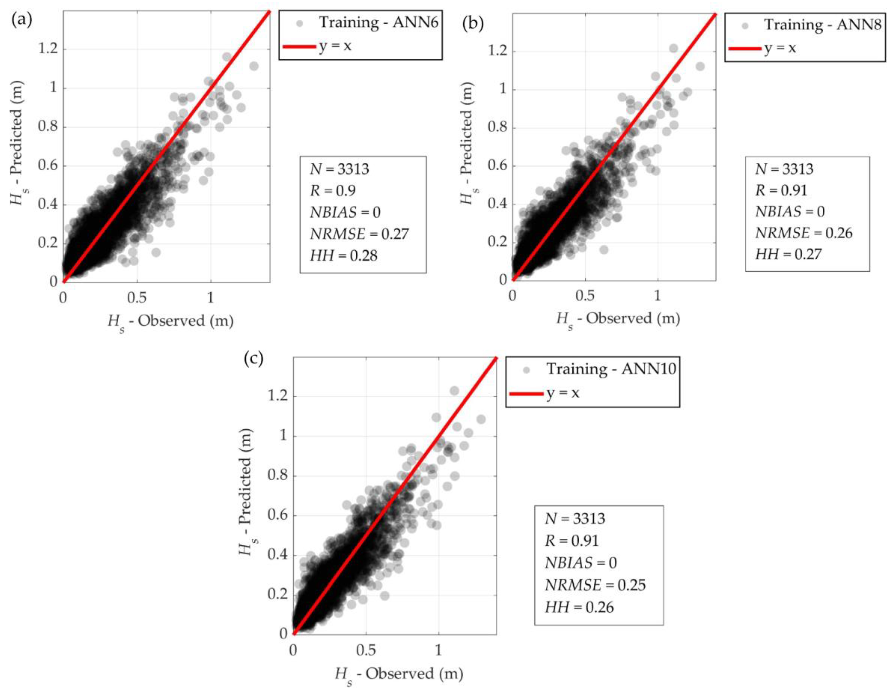
3.2. Training of ANN

The training procedure was performed as described in Section 2.3, using 80% of the available data points from 1 November 2007 to 19 June 2008, while the remaining 20% was used to test filling the missing data points of significant wave height. Figure 6 shows that increasing the features from ANN6 to ANN10 only slightly increased the accuracy of ANN on the training set (from ANN6 to ANN10; HH decreases by 7%). However, this is not a measure of the overall ANN accuracy, but could indicate possible overfitting.
We repeated the random separation of the training set and the test set labeled as ‘missing’ (described in detail in Section 2.3) 10 times to observe the sensitivity of the accuracy of the model ANN to the random separation. This was tested with the ANN10 model, and the results generally showed low sensitivity (Figure 7). The sensitivity to random separation was higher for the training sets with larger standard deviations than for the two test sets, except for the NBIAS, where the situation was reversed. The mean HH and NRMSE indices were slightly higher in the test sets than in the training sets, while the R index was slightly lower than in the training sets, both of which were to be expected.
Although the model performance indices varied little for different random training and test separations (Figure 7), Table 5 shows the hyperparameters of the trained ANNs which performed best during the five-fold cross-validation training. Interestingly, all ANNs trained best with similar hyperparameters (Table 4). Relu was chosen as the best activation function, in combination with only one relatively broad hidden layer (113, 287, and 296 for ANN6, ANN8, and ANN10, respectively). The regularization term, the lambda value, increased with the increase of features to a value of about double (from ANN6 to ANN10).

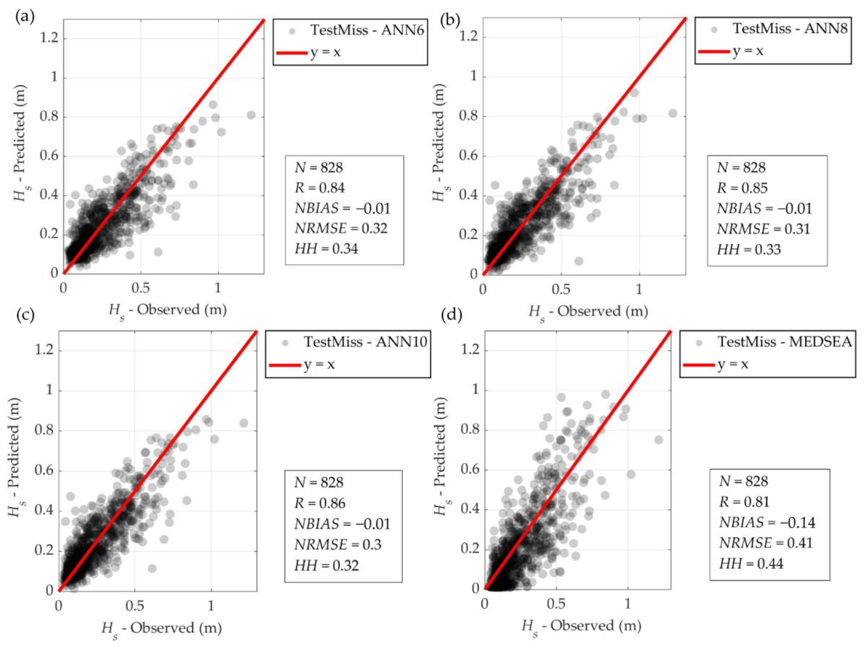
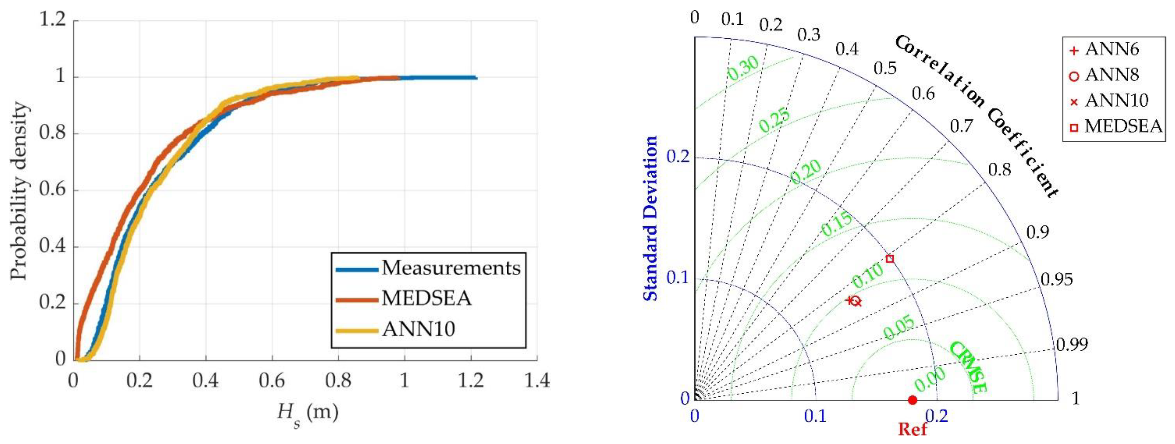
3.3. Filling Missing Wave Data Using an ANN

Filling the missing wave data points with the MEDSEA reanalysis wave model showed relatively poor results compared to the filling capabilities of trained ANNs (Figure 8). The error of filling wave data points with MEDSEA (HH = 0.44) was 37.5% higher than that of ANN10 (HH = 0.32). The ANNs with a smaller number of features, ANN6 and ANN8, showed slightly worse accuracy than ANN10 (HH index decrease of 6% and 3%, respectively). However, they still showed significantly lower error than the fill procedure using MEDSEA reanalysis wave data (29% and 33% for ANN6 and ANN8, respectively).
The correct wave buoy data points were moderately underpredicted (14%) by the MEDSEA reanalysis (Figure 8). MEDSEA predominantly underpredicted the smaller observed significant wave heights Hs < 0.25 m, while it mostly overpredicted the higher significant wave heights Hs > 0.5 m. On the other hand, every ANN showed minor underprediction (−1% for ANN6, ANN8 and ANN10).
The empirical Cumulative Distribution Functions (CDFs) in Figure 9 (left) again show better agreement between the wave data reconstructed by ANN10 and the correct (measured) significant wave heights. The CDF for MEDSEA shows a higher probability density for significant wave heights below 0.4 m, with the curves intersecting at 0.5 m and showing a lower probability density thereafter. The high probability density of the MEDSEA CDF is due to a strong underprediction of low significant wave heights (Hs < 0.4 m) also observed in Figure 8d. On the other hand, the CDF of ANN10 shows greater agreement with measurements for the entire range of significant wave heights. Both MEDSEA and ANN10 CDF fall short of the highest observed significant wave height, indicating underprediction in the highest observed value. The Taylor diagram in Figure 9 (right) again shows that the accuracy of the ANN models (ANN6, ANN8 and ANN10) are very similar, while still showing superior accuracy as opposed to the state-of-the-art reanalysis wave model, MEDSEA.

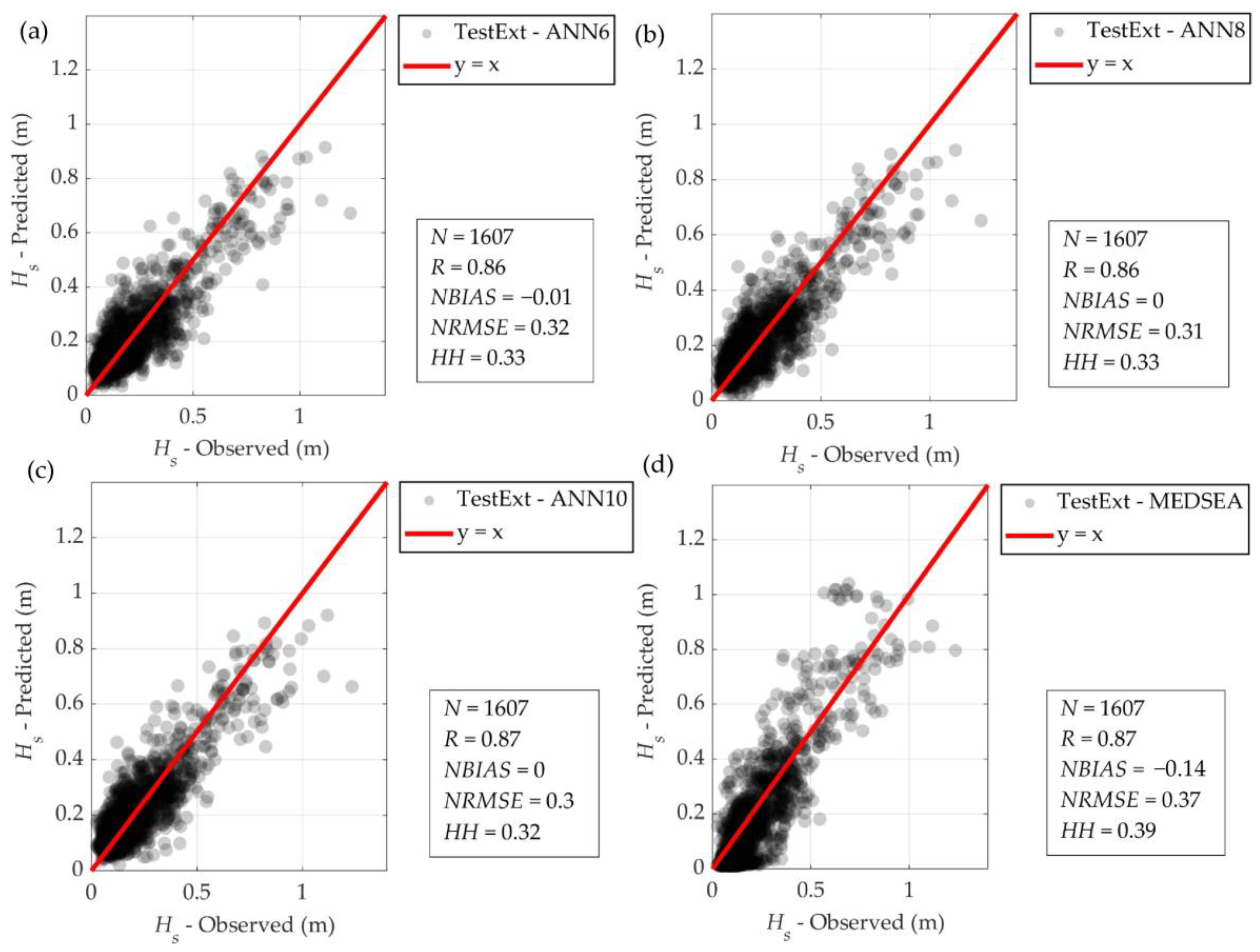
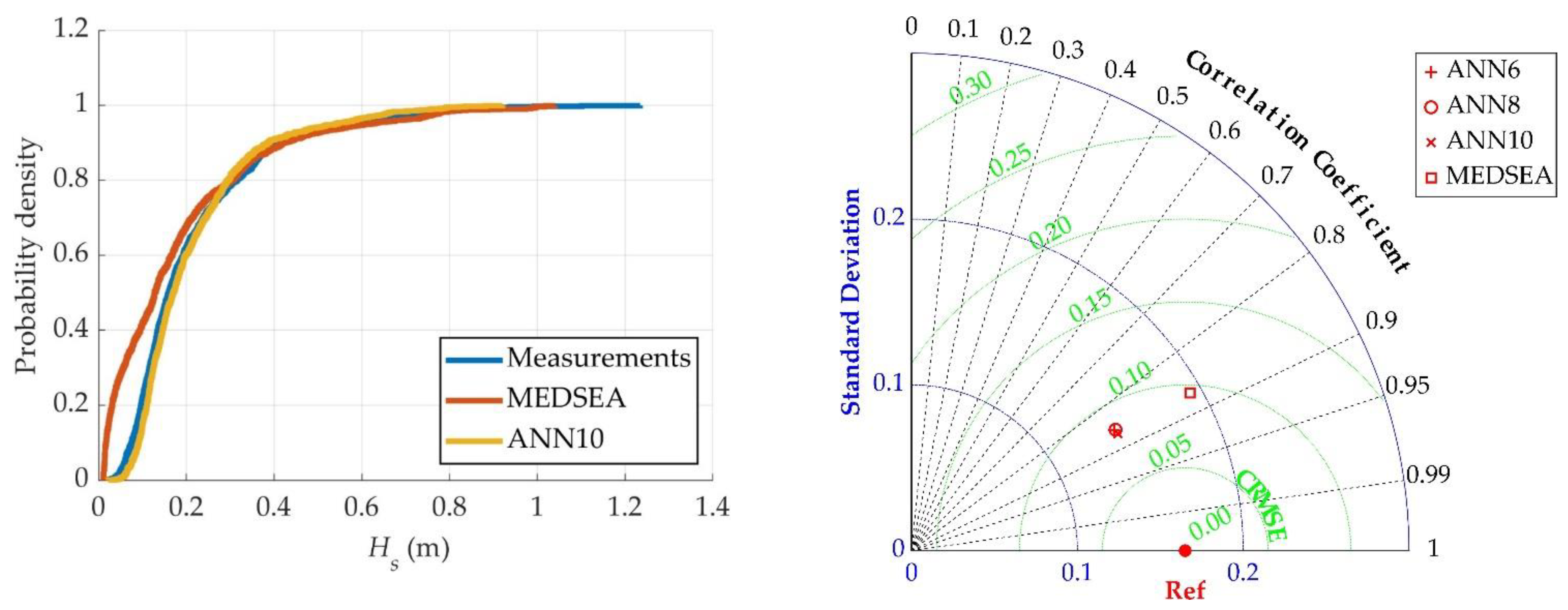
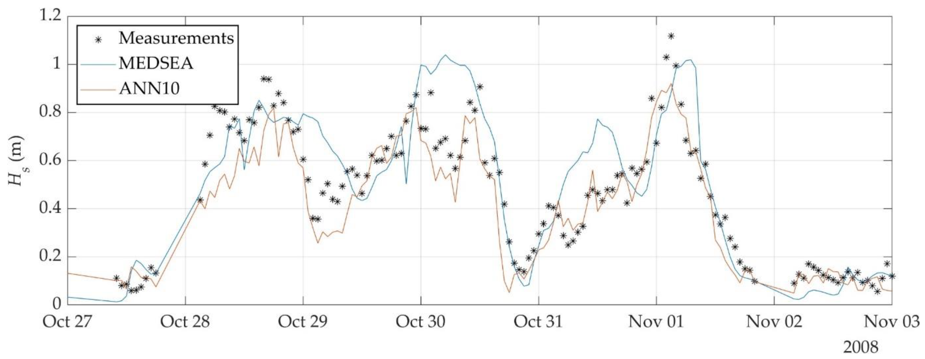
3.4. Extension of Wave Data Using a Trained ANN

Figure 10 shows the accuracy of the ANNs and MEDSEA reanalysis wave data with respect to the measured significant wave heights outside the training period from 8 August 2008 to 15 November 2008 (limits shown with blue vertical lines in Figure 2).
A similar pattern of ANN accuracy is observed for wave extension (Figure 10) as for filling in the missing wave data in Section 3.3. As the number of features in ANN increased, the error decreases slightly (by 3% from ANN6 to ANN10). However, each ANN still shows greater accuracy compared to the wave data from the MEDSEA reanalysis model. The HH index increased by 22% when the MEDSEA reanalysis data were used instead of the reconstructed wave data from ANN. The MEDSEA reanalysis still underestimated the wave buoy measurements (NBIAS = −14%), while the ANNs showed minor underestimation or no bias (NBIAS = −1% for ANN6 and no bias at all for ANN8 and ANN10).
Figure 11 (left) shows the empirical CDF for the measured significant wave heights in the testing period for wave data extension, as described in Section 2.2. The ANN reconstructed wave data again showed better agreement with the measured data, as opposed to the MEDSEA. This was especially evident in the region of low observed significant wave heights Hs < 0.4 m, where the MEDSEA probability density was substantially higher than the measured one. Both MEDSEA and ANN10 CDF fell short of the highest observed significant wave height, indicating underprediction of the peak significant wave heights. The Taylor diagram in Figure 11 (right) again shows that the accuracy of the ANN models (ANN6, ANN8 and ANN10) are very similar, as was the case when testing the accuracy to fill missing wave data (Section 3.3), while still showing slightly better accuracy as opposed to the state-of-the-art reanalysis wave model, MEDSEA.
The time series excerpt shown in Figure 12 illustrates the ability of ANN to follow the trend of measured significant wave heights. The agreement between ANN and the measured wave heights was stronger compared to the MEDSEA reanalysis data, especially when the wave heights showed a downward trend (e.g., early October 29 and 30). However, the ANN showed poorer agreement in situations with local maxima of significant wave heights, such as on November 1, when the ANN reconstructed wave heights tended to underpredict the peak values.

4. Discussion

In contrast to previous findings by Vieira, Cavalcante [34], who assumed that wind data was not an essential parameter in the ANN training procedure, these results suggest that wind in itself can provide reasonable accuracy to fill in missing wave data or an extension of wave data outside the training period. It should be noted that Vieira and Cavalcante [34] also used wave reanalysis data as an input feature for ANN, which have greater explanatory power compared to wind data and therefore overshadowed the explanatory power of wind data. Moreover, the wind data used in [34] were obtained from a reanalysis model and were not measured directly at weather stations, as in this study. Therefore, it could be assumed that the reanalysis wind data did not have the same importance as the measured wind data. On the other hand, Shamshirband, Mosavi [36] have shown that wind data, even from the reanalysis models, can be sufficient for an effective machine learning model, which is consistent with this study.
Mahjoobi and Adeli Mosabbeb [27] cautioned that ANN in wave prediction applications might overfit the training data, which could reduce the accuracy of ANN on the test set, but this was not observed in this study. As the number of features increased, accuracy increased on both the training (Figure 5) and test (Figure 6 and Figure 8) sets. However, this increase in accuracy was only slight; specifically, HH decreased by 6% from ANN6 to ANN10 in the missing wave data test.
The accuracy of ANN for filling missing wave data (Section 3.3) and extending wave data beyond the training period (Section 3.4) was similar (if ANN10 is used the HH was the same; HH = 0.32 for both wave filling and wave extension, respectively). This indicates that the same ANN could be used to further extend the measured wave data without significantly decreasing accuracy. Nevertheless, this should be confirmed in future studies with wave measurements at least several years away from the training period. However, as the results show for both filling in missing wave data and expanding wave data, the ANN methods tend to underpredict the higher observed significant wave heights (Hs > 0.7 m). This could be due to a higher number of lower significant wave heights (Hs < 0.5 m) In the measurements, and therefore in the training and testing sets. The ANN training procedure therefore adjusts the ANN’s node weights and biases in order to minimize the error for the majority of wave data, which in the case of Split, Croatia, are the low significant wave heights. For occasional higher wave heights, the trained ANN does not focus on reconstructing these rare cases, as opposed to the low significant wave heights that make up the majority of the data points. In the future, the input data for the ANN could be pre-filtered to exclude or limit the number of data points with low significant wave heights, or strong weights could be introduced to the loss function of ANN to increase the importance of errors for predicting higher significant wave heights.
In agreement with the report of Korres, Ravdas [23], the MEDSEA model showed relatively low accuracy when validating the reanalysis data with buoy measurements off Split, a well-protected area. This accuracy comparison can be seen in Figure 6 and Figure 8. This degradation in reanalysis accuracy is likely due to the relatively large numerical cell size of the reanalysis model. In these situations, local numerical wave models could be used through the downscaling procedure for a detailed numerical description and an overall increase in accuracy [17,19].
This study was limited to the use of the publicly available Integrated Surface Database [38,39,40], which is itself riddled with missing data, as shown in Section 2.2 and Section 3.1. The cleaning procedure remedied this to some extent, but the authors assume that ANNs trained on complete and more detailed weather data from the National Weather Service would have even better accuracy. This should be confirmed in a future study. Even though the quality of the wind data was not optimal, the trained ANN showed much better accuracy compared to the MEDSEA reanalysis (Figure 6 and Figure 8). As reported by Korres, Ravdas [23], this relatively low accuracy of MEDSEA was probably due to the complex topography and the limited resolution of the wave model. This is all because the eastern Adriatic is a basin that is predominantly semi-enclosed by islands.

5. Conclusions

In this work, ANNs were constructed and trained to test their ability to fill in missing wave data or extend the measured wave data. Different hyperparameter settings and input features were varied to find a robust framework for ANN construction and training.
Univariate feature ranking was performed to select the most relevant input features from weather data publicly available as part of NOAA’s Integrated Surface Database. The analysis revealed that the most important input features were wind magnitude and direction data collected from weather stations near the location of the wave buoy, while data from more distant weather stations had little predictive power and were therefore excluded from the set of input features. Weather data such as air temperature, dew point, relative humidity, and air pressure also had low predictive power, and were therefore also excluded from the feature set.
Based on the univariate feature ranking, ANNs were constructed from the first 6, 8, and 10 ranked features (which were exclusively wind velocity magnitude and wind direction from nearby weather stations, see Table 4) to see if additional features increased the accuracy of ANN. Increasing the number of features from 6 to 10 showed a slight improvement, both in testing the filling of missing wave data and in expanding wave data outside the original measurement period. Therefore, ANNs constructed with a smaller number of input features are preferred to reduce model complexity. In addition, the framework using Bayesian optimization was found to be robust, as the accuracy of ANN on test data showed low sensitivity to the separation of training and test data, while the hyperparameter settings were consistently similar. The hyperparameters identified were consistently the relu activation function and a broad hidden layer (113 to 296 nodes in the hidden layer for a decreasing number of input features from ANN10 to ANN6).
When testing the ANNs on the test data for filling missing wave data and extending wave data beyond the original measurement period, the accuracy is similar (ANN10 showed a scatter of HH = 0.32 and HH = 0.32 and a correlation of R = 0.87 and R = 0.86 for filling missing wave data and extending wave data, respectively). Interestingly, the ANNs showed higher accuracy than a state-of-the-art publicly available reanalysis wave model for the Mediterranean Sea, MEDSEA (provided by Copernicus Marine Service). The MEDSEA reanalysis data points showed a 22% increase in HH for expanding wave data and a 33% increase in HH for filling wave data points. This benchmark against MEDSEA demonstrated that the ANN’s accuracy was reliable. Overall, the paper results demonstrated that a robust method for constructing ANNs based on publicly collected wind strengths and directions can accurately fill in missing wave data and expand wave data beyond the original training period.
The inherent value of machine learning methods in this case should be noted, as they are faster and do not require hard-to-obtain values such as bathymetry and white-capping parameters, as is the case with numerical wave modeling.

Author Contributions

Conceptualization, D.B.; methodology, D.B., T.B. and D.C.; software, D.B.; validation, D.B., T.B. and D.C.; formal analysis, D.B. and H.M.; investigation, D.B., T.B. and H.M.; resources, D.C.; data curation, T.B. and H.M.; writing—original draft preparation, D.B. and T.B.; writing—review and editing, D.B., T.B., D.C. and H.M.; visualization, D.B. and H.M.; supervision, D.C.; project administration, D.C. All authors have read and agreed to the published version of the manuscript.

Funding

This research received no external funding.

Institutional Review Board Statement

Not applicable.

Informed Consent Statement

Not applicable.

Data Availability Statement

The data presented in this study are available on request from the corresponding author.

Conflicts of Interest

The authors declare no conflict of interest. The funders had no role in the design of the study; in the collection, analyses, or interpretation of data; in the writing of the manuscript; or in the decision to publish the results.

References

  1. Nitsure, S.P.; Londhe, S.N.; Khare, K.C. Wave forecasts using wind information and genetic programming. Ocean Eng. 2012, 54, 61–69. [Google Scholar] [CrossRef]
  2. Ojo, A.; Collu, M.; Coraddu, A. Multidisciplinary design analysis and optimization of floating offshore wind turbine substructures: A review. Ocean Eng. 2022, 266, 112727. [Google Scholar] [CrossRef]
  3. Goda, Y. Random Seas and Design of Maritime Structure; University of Tokyo Press: Tokyo, Japan, 1985. [Google Scholar]
  4. Bosom, E.; Jimenez, J.A. Probabilistic coastal vulnerability assessment to storms at regional scale—Application to Catalan beaches (NW Mediterranean). Nat. Hazards Earth Syst. Sci. 2011, 11, 475–484. [Google Scholar] [CrossRef] [Green Version]
  5. IEA. Renewable Power; IEA: Paris, France, 2022. [Google Scholar]
  6. Sacie, M.; Santos, M.; López, R.; Pandit, R. Use of State-of-Art Machine Learning Technologies for Forecasting Offshore Wind Speed, Wave and Misalignment to Improve Wind Turbine Performance. J. Mar. Sci. Eng. 2022, 10, 938. [Google Scholar] [CrossRef]
  7. Robertson, B.; Dunkle, G.; Gadasi, J.; Garcia-Medina, G.; Yang, Z.Q. Holistic marine energy resource assessments: A wave and offshore wind perspective of metocean conditions. Renew. Energy 2021, 170, 286–301. [Google Scholar] [CrossRef]
  8. Wu, M.N.; Stefanakos, C.; Gao, Z. Multi-Step-Ahead Forecasting of Wave Conditions Based on a Physics-Based Machine Learning (PBML) Model for Marine Operations. J. Mar. Sci. Eng. 2020, 8, 992. [Google Scholar] [CrossRef]
  9. Bahaghighat, M.; Abedini, F.; Xin, Q.; Zanjireh, M.M.; Mirjalili, S. Using machine learning and computer vision to estimate the angular velocity of wind turbines in smart grids remotely. Energy Rep. 2021, 7, 8561–8576. [Google Scholar] [CrossRef]
  10. Vannucchi, V.; Taddei, S.; Capecchi, V.; Bendoni, M.; Brandini, C. Dynamical Downscaling of ERA5 Data on the North-Western Mediterranean Sea: From Atmosphere to High-Resolution Coastal Wave Climate. J. Mar. Sci. Eng. 2021, 9, 208. [Google Scholar] [CrossRef]
  11. Peres, D.J.; Iuppa, C.; Cavallaro, L.; Cancelliere, A.; Foti, E. Significant wave height record extension by neural networks and reanalysis wind data. Ocean Model. 2015, 94, 128–140. [Google Scholar] [CrossRef]
  12. World Meteorological Organization. Guide to Wave Analysis and Forecasting; WMO: Geneva, Switzerland, 2018; Volume WMO-No. 702. [Google Scholar]
  13. Goda, Y. Revisiting Wilson’s formulas for simplified wind-wave prediction. J. Waterw. Port Coast. Ocean Eng. 2003, 129, 93–95. [Google Scholar] [CrossRef]
  14. WAMDI Group. The WAM Model—A Third Generation Ocean Wave Prediction Model. J. Phys. Oceanogr. 1988, 18, 1775–1810. [Google Scholar] [CrossRef]
  15. Booij, N.; Ris, R.C.; Holthuijsen, L.H. A third-generation wave model for coastal regions: 1. Model description and validation. J. Geophys. Res. Ocean. 1999, 104, 7649–7666. [Google Scholar] [CrossRef] [Green Version]
  16. Smith, C.A.; Compo, G.P.; Hooper, D.K. Web-Based Reanalysis Intercomparison Tools (WRIT) for Analysis and Comparison of Reanalyses and Other Datasets. B. Am. Meteorol. Soc. 2014, 95, 1671–1678. [Google Scholar] [CrossRef]
  17. Bellotti, G.; Franco, L.; Cecioni, C. Regional Downscaling of Copernicus ERA5 Wave Data for Coastal Engineering Activities and Operational Coastal Services. Water 2021, 13, 859. [Google Scholar] [CrossRef]
  18. Feng, X.; Chen, X. Feasibility of ERA5 reanalysis wind dataset on wave simulation for the western inner-shelf of Yellow Sea. Ocean Eng. 2021, 236, 109413. [Google Scholar] [CrossRef]
  19. Bujak, D.; Loncar, G.; Carevic, D.; Kulic, T. The Feasibility of the ERA5 Forced Numerical Wave Model in Fetch-Limited Basins. J. Mar. Sci. Eng. 2023, 11, 59. [Google Scholar] [CrossRef]
  20. Kim, S.; Tom, T.H.A.; Takeda, M.; Mase, H. A framework for transformation to nearshore wave from global wave data using machine learning techniques: Validation at the Port of Hitachinaka, Japan. Ocean Eng. 2021, 221, 108516. [Google Scholar] [CrossRef]
  21. Hersbach, H.; Bell, B.; Berrisford, P.; Hirahara, S.; Horanyi, A.; Munoz-Sabater, J.; Nicolas, J.; Peubey, C.; Radu, R.; Schepers, D.; et al. The ERA5 global reanalysis. Q. J. Roy. Meteor. Soc. 2020, 146, 1999–2049. [Google Scholar] [CrossRef]
  22. Law-Chune, S.; Aouf, L.; Dalphinet, A.; Levier, B.; Drillet, Y.; Drevillon, M. WAVERYS: A CMEMS global wave reanalysis during the altimetry period. Ocean Dyn. 2021, 71, 357–378. [Google Scholar] [CrossRef]
  23. Korres, G.; Ravdas, M.; Zacharioudaki, A. Mediterranean Sea Waves Hindcast (CMEMS MED-Waves); CMEMS, Ed.; CMEMS: Ramonville-Saint-Agne, France, 2019. [Google Scholar] [CrossRef]
  24. Haykin, S. Neural Networks: A Comprehensive Foundation, 1999; Prentice Hall: Mcmillan, NJ, USA, 2010; pp. 1–24. [Google Scholar]
  25. Berbić, J.; Ocvirk, E.; Carević, D.; Lončar, G. Application of neural networks and support vector machine for significant wave height prediction. Oceanologia 2017, 59, 331–349. [Google Scholar] [CrossRef]
  26. Elbisy, M.S.; Elbisy, A.M.S. Prediction of significant wave height by artificial neural networks and multiple additive regression trees. Ocean Eng. 2021, 230, 109077. [Google Scholar] [CrossRef]
  27. Mahjoobi, J.; Adeli Mosabbeb, E. Prediction of significant wave height using regressive support vector machines. Ocean Eng. 2009, 36, 339–347. [Google Scholar] [CrossRef]
  28. Mahjoobi, J.; Etemad-Shahidi, A.; Kazeminezhad, M.H. Hindcasting of wave parameters using different soft computing methods. Appl. Ocean Res. 2008, 30, 28–36. [Google Scholar] [CrossRef]
  29. Passarella, M.; Goldstein, E.B.; De Muro, S.; Coco, G. The use of genetic programming to develop a predictor of swash excursion on sandy beaches. Nat. Hazards Earth Syst. Sci. 2018, 18, 599–611. [Google Scholar] [CrossRef] [Green Version]
  30. van Maanen, B.; Coco, G.; Bryan, K.R.; Ruessink, B.G. The use of artificial neural networks to analyze and predict alongshore sediment transport. Nonlinear Proc. Geoph. 2010, 17, 395–404. [Google Scholar] [CrossRef]
  31. Goldstein, E.B.; Coco, G.; Plant, N.G. A review of machine learning applications to coastal sediment transport and morphodynamics. Earth-Sci. Rev. 2019, 194, 97–108. [Google Scholar] [CrossRef] [Green Version]
  32. Bujak, D.; Bogovac, T.; Carević, D.; Ilic, S.; Lončar, G. Application of Artificial Neural Networks to Predict Beach Nourishment Volume Requirements. J. Mar. Sci. Eng. 2021, 9, 786. [Google Scholar] [CrossRef]
  33. Londhe, S.N. Soft computing approach for real-time estimation of missing wave heights. Ocean Eng. 2008, 35, 1080–1089. [Google Scholar] [CrossRef]
  34. Vieira, F.; Cavalcante, G.; Campos, E.; Taveira-Pinto, F. A methodology for data gap filling in wave records using Artificial Neural Networks. Appl. Ocean Res. 2020, 98, 102109. [Google Scholar] [CrossRef]
  35. Alexandre, E.; Cuadra, L.; Nieto-Borge, J.C.; Candil-García, G.; del Pino, M.; Salcedo-Sanz, S. A hybrid genetic algorithm—Extreme learning machine approach for accurate significant wave height reconstruction. Ocean Model. 2015, 92, 115–123. [Google Scholar] [CrossRef]
  36. Shamshirband, S.; Mosavi, A.; Rabczuk, T.; Nabipour, N.; Chau, K.-w. Prediction of significant wave height; comparison between nested grid numerical model, and machine learning models of artificial neural networks, extreme learning and support vector machines. Eng. Appl. Comput. Fluid Mech. 2020, 14, 805–817. [Google Scholar] [CrossRef]
  37. Kim, T.; Lee, W.-D. Review on Applications of Machine Learning in Coastal and Ocean Engineering. J. Ocean Eng. Technol. 2022, 36, 194–210. [Google Scholar] [CrossRef]
  38. Smith, A.; Lott, N.; Vose, R. The Integrated Surface Database Recent Developments and Partnerships. B. Am. Meteorol. Soc. 2011, 92, 704–708. [Google Scholar] [CrossRef] [Green Version]
  39. Lott, N.; Vose, R.; Del Greco, S.A.; Ross, T.F.; Worley, S.J.; Comeaux, J. The integrated surface database: Partnerships and progress. In Proceedings of the 24th Conference on Interactive Information Processing Systems for Meteorology, Oceanography and Hydrology, New Orleans, LA, USA, 20 January 2008. [Google Scholar]
  40. Lott, J.N. The quality control of the integrated surface hourly database. In Proceedings of the 14th Conference on Applied Climatology, Seattle, WA, USA, 10–15 January 2004. [Google Scholar]
  41. Komen, G.J.; Cavaleri, L.; Donelan, M.; Hasselmann, K.; Hasselmann, S.; Janssen, P. Dynamics and Modelling of Ocean Waves; Cambridge University Press: Cambridge, UK, 1994. [Google Scholar]
  42. Janssen, P.A.E.M. Wave-Induced Stress and the Drag of Air Flow over Sea Waves. J. Phys. Oceanogr. 1989, 19, 745–754. [Google Scholar] [CrossRef]
  43. Janssen, P. Quasi-linear Theory of Wind-Wave Generation Applied to Wave Forecasting. J. Phys. Oceanogr. 1991, 21, 1631–1642. [Google Scholar] [CrossRef]
  44. Hasselmann, K. On the spectral dissipation of ocean waves due to white capping. Bound.-Layer Meteorol. 1973, 6, 107–127. [Google Scholar] [CrossRef]
  45. Weatherall, P.; Marks, K.M.; Jakobsson, M.; Schmitt, T.; Tani, S.; Arndt, J.E.; Rovere, M.; Chayes, D.; Ferrini, V.; Wigley, R. A new digital bathymetric model of the world’s oceans. Earth Space Sci. 2015, 2, 331–345. [Google Scholar] [CrossRef]
  46. Lionello, P.; Gunther, H.; Janssen, P.A.E.M. Assimilation of Altimeter Data in a Global 3rd-Generation Wave Model. J. Geophys. Res. Ocean. 1992, 97, 14453–14474. [Google Scholar] [CrossRef]
  47. van Gent, M.R.A.; van den Boogaard, H.F.P.; Pozueta, B.; Medina, J.R. Neural network modelling of wave overtopping at coastal structures. Coast. Eng. 2007, 54, 586–593. [Google Scholar] [CrossRef] [Green Version]
  48. Nocedal, J.; Wright, S.J. Numerical Optimization, 2nd ed.; Jorge, N., Ed.; Springer: New York, NY, USA, 2006. [Google Scholar]
  49. Hanna, S.R.; Heinold, D.W. Development and Application of a Simple Method for Evaluating Air Quality; American Petroleum Institute, Health and Environmental Affairs Department: Washington, DC, USA, 1985. [Google Scholar]
  50. Mentaschi, L.; Besio, G.; Cassola, F.; Mazzino, A. Problems in RMSE-based wave model validations. Ocean Model. 2013, 72, 53–58. [Google Scholar] [CrossRef]
Figure 1. Map of the study site on the southern coast of Croatia, showing nine weather stations (circles) and one wave buoy (rectangle), described in detail in Section 2.2.
Wind 03 00010 g001
Figure 2. Time series of measured significant wave heights at the wave buoy location in front of Split with indicated period for ANN training and ANN testing for filling missing data (limited by red vertical lines) and period for ANN testing for wave data extension (limited by blue vertical lines).
Wind 03 00010 g002
Figure 3. Workflow of the ANN model building and testing.
Wind 03 00010 g003
Figure 4. Schematic diagram of a feed-forward neural network constructed for filling in missing wave data or extending wave data.
Wind 03 00010 g004
Figure 5. Univariate feature ranking of each predictor from the ISD weather database (described in Section 2.2) using an F-test; orange bars indicate that the predictor score is actually Inf, but are scaled to the largest non-Inf (blue) score.
Wind 03 00010 g005
Figure 6. Statistical error metrics for evaluating ANN accuracy on the training set for the (a) ANN6, (b) ANN8, and (c) ANN10 (description of ANN shown in Table 3).
Wind 03 00010 g006
Figure 7. Box plots of trained ANN10 models using 10 different random separations for the training set and test set for testing the filling of missing data.
Wind 03 00010 g007
Figure 8. Statistical error metrics for evaluating ANN accuracy for filling missing wave data points on the test set for (a) ANN6, (b) ANN8, and (c) ANN10 (description of ANN shown in Table 3), and MEDSEA reanalysis model accuracy on (d) MEDSEA.
Wind 03 00010 g008
Figure 9. (left) Empirical CDF comparing measurements for the missing wave data points with ANN10 reconstructed wave data and MEDSEA reanalysis wave data; (right) Taylor diagram comparing the accuracy of the models for filling missing wave data.
Wind 03 00010 g009
Figure 10. Statistical error metrics for evaluating ANN accuracy for extending wave data points beyond the original measuring period for (a) ANN6, (b) ANN8, and (c) ANN10 (description of ANN shown in Table 3), and MEDSEA reanalysis model accuracy on (d) MEDSEA.
Wind 03 00010 g010
Figure 11. (left) Empirical CDF comparing measurements with ANN10 reconstructed wave data and MEDSEA reanalysis wave data for the extension of wave data points; (right) Taylor diagram comparing the accuracy of the models for wave data extension.
Wind 03 00010 g011
Figure 12. Time series excerpt of measured wave parameters at wave buoy location in front of Split (Figure 1), modeled MEDSEA reanalysis wave data, and ANN10 reconstructed wave data.
Wind 03 00010 g012
Table 1. Measured meteorological features obtained from ISD for the 9 locations shown in Figure 1 and Table 2 (items 2–10), which were used as inputs in the artificial neural network.
Feature NamePhysical Measure (Units)
tempAir temperature (°C)
dewDew point (°C)
rhumRelative humidity (%)
wdirWind direction (°)
wmagWind magnitude (km/h)
presSea-level air pressure (hPa)
Table 2. The sources of wave and wind data used in the study, with the respective spatial and temporal resolutions.
Wind DataTypeSpatial ResolutionTemporal ResolutionLocation/RegionAltitude
MEDSEAGridded data (Copernicus)0.25° × 0.25°1 hRegional, extracted at wave buoy locationN/A
HvarWeather data (ISD)Point data1 h43° 10′ 15″ N
16° 26′ 14″ E
20 m
ResnikWeather data (ISD)Point data1 h43° 32′ 22″ N
16° 18′ 5″ E
19 m
SplitWeather data (ISD)Point data1 h43° 30′ 30″ N
16° 25′ 35″ E
122 m
LastovoWeather data (ISD)Point data1 h42° 46′ 6″ N
16° 54′ 1″ E
186 m
PalagruzaWeather data (ISD)Point data1 h42° 23′ 36″ N
16° 15′ 05″ E
98 m
KomizaWeather data (ISD)Point data1 h43° 2′ 55″ N
16° 5′ 14″ E
20 m
SibenikWeather data (ISD)Point data1 h43° 43′ 41″ N
15° 54′ 23″ E
77 m
PloceWeather data (ISD)Point data1 h43° 2′ 51″ N
17° 26′ 34″ E
2 m
MakarskaWeather data (ISD)Point data1 h43° 17′ 16″ N
17° 1′ 12″ E
50 m
Table 3. Wave and wind data sources used in this study with corresponding spatial and temporal resolutions.
FeatureAvailable Data Points
Hvar98%
Komiza98%
Lastovo32%
Makarska61%
Palagruza16%
Ploce61%
Resnik99%
Sibenik98%
Split99%
Table 4. Input features used for training the ANNs with 6, 8, and 10 input features; features are ordered by predictor importance (Figure 5); the mark ‘x’ designates the features that are included in the respective ANN, and the mark ‘-‘ designates the features not included in the respective ANN.
ANNANN6ANN8ANN10
wmag_Hvarxxx
wmag_Komizaxxx
wmag_Makarskalow amount of data points
wdir_Resnikxxx
wmag_Resnikxxx
wmag_Sibenikxxx
wmag_Splitxxx
wdir_Split-xx
wmag_Lastovolow amount of data points
wdir_Hvar-xx
wdir_Komiza--x
wmag_Plocelow amount of data points
wdir_Sibenik--x
Table 5. Hyperparameters inside the ANN training procedure that showed the best accuracy.
ANNActivation FunctionLambdaHidden Layers
ANN6 (Figure 6a)relu0.00039296
ANN8 (Figure 6b)relu0.00055297
ANN10 (Figure 6c)relu0.00060113
Disclaimer/Publisher’s Note: The statements, opinions and data contained in all publications are solely those of the individual author(s) and contributor(s) and not of MDPI and/or the editor(s). MDPI and/or the editor(s) disclaim responsibility for any injury to people or property resulting from any ideas, methods, instructions or products referred to in the content.

