Switching Kalman Filtering-Based Corrosion Detection and Prognostics for Offshore Wind-Turbine Structures

Abstract

Since manual inspections of offshore wind turbines are costly, there is a need for remote monitoring of their health condition, including health prognostics. In this paper, we focus on corrosion detection and corrosion prognosis since corrosion is a major failure mode of offshore wind turbine structures. In particular, we propose an algorithm for corrosion detection and three algorithms for corrosion prognosis by using Bayesian filtering approaches, and quantitatively compare their accuracy against synthetic datasets having characteristics typical for wall thickness measurements using ultrasound sensors. We found that a corrosion prognosis algorithm based on the Pourbaix corrosion model using unscented Kalman filtering outperforms the algorithms based on a linear corrosion model and the bimodal corrosion model introduced by Melchers.

1. Introduction

New wind farms are often operating far from shore and under challenging and highly-corrosive operating conditions. To reduce the number of regular manual inspections, remote monitoring of the health condition of critical components and sub-systems in offshore wind turbines is necessary [1]. Moreover, for decommissioning and maintenance scheduling, prognosis of the remaining useful life of wind turbines is essential.

Corrosion, and in particular uniform corrosion, is a major cause of failure of offshore structures [2,3]. Indeed, uniform corrosion may reduce the steel wall of the wind turbine structure beyond its corrosion allowance, at which point the structure reaches the end of useful life. The thickness of the steel wall of the wind turbine structure can be continuously measured using ultrasound sensors mounted on the interior side of the wall [4,5] and corrosion information (including corrosion prognosis) can then be visualized for the onshore wind farm operator [6]. We remark that ultrasound is but one possible technique to monitor corrosion, see, e.g., [7], where electrochemical techniques are used instead of ultrasound. In this paper, we focus on ultrasound due to its attractive trade-off between measurement accuracy and cost [5]. Moreover, we remark that the sensors need not be fixed, but can be equipped on climbing robots, UAVs, or underwater robots [8].

A typical corrosion prognosis method uses historical offline data only to estimate the unknown parameters of an empirical corrosion model, see, e.g., [9,10]. Similarly to in [11,12], we focus in this paper on corrosion prognosis of offshore wind-turbine structures using real-time measurement data. Corrosion prognosis is an essential component within a decision support pipeline where an optimal decommissioning time can be computed depending on the cost of operations and maintenance, energy production, risk aversion, etc. [13].

We present a corrosion detection method and three corrosion prognosis methods based on a technique called Bayesian filtering [14], following an approach as outlined in a high-level in [15]. The corrosion detection method identifies the onset of corrosion, i.e., the initial wall thickness reduction when the coating (at the monitored position) is fully degraded and the bare steel is exposed. The corrosion prognosis algorithms compute the probability distribution of the remaining useful life time. Each corrosion prognosis algorithm is based on a particular corrosion model. In particular, we consider the linear corrosion model, the power-law corrosion model, and the involved bimodal corrosion model [16]. The prognosis algorithms are compared using the well-known remaining useful life $\alpha$-$\lambda$-accuracy metric against synthetic datasets having measurement and process noise levels typical for wall thickness measurements using ultrasound sensors.

A conference version of this paper containing preliminary results is published in the conference proceedings of IWSHM 2021 [17]. More specifically, the present paper (1) considers coated steel (as opposed to bare steel in the conference paper), thereby introducing a corrosion detection phase, (2) considers prognosis methods based on three degradation models (the power-law model was not considered in the conference paper), and (3) provides quantitative (i.e., based on metrics), as opposed to qualitative, performance results.

This paper is structured as follows. Section 2 discusses Bayesian filtering, including Kalman filtering and extensions of Kalman filtering, and in Section 3 we discuss the proposed methodology, consisting of a corrosion detection phase followed by a corrosion prognosis phase. The accuracy performance of the proposed methods against the synthetic datasets is evaluated in Section 4. Finally, we provide a conclusion in Section 5.

2. Bayesian Filtering

While prognosis of a wind turbine structure can be based solely on the current lifetime of the wind turbine and historical data (e.g., the mean useful lifetime of offshore wind turbines), one can improve the accuracy of the remaining useful life prognosis by using online measurements. Since there is currently a very limited amount of historical data available on corrosion of offshore wind turbine structures covering the entire lifetime from commissioning until end of life, using data-driven methods (such as typical AI-based methods) for corrosion detection and prognosis are likely currently unsuitable, i.e., give inaccurate results for newly acquired measurement datapoints. Instead, we employ a well-known technique called Bayesian filtering [14]. In Bayesian filtering, an empirical corrosion model, describing the amount of corrosion loss over time, is used together with online measurements to estimate the unknown parameters of the model. Process noise (i.e., the inaccuracy of the corrosion model) and measurement noise (i.e., the inaccuracy of the measurements) are both taken into account in Bayesian filtering.

In general, Bayesian filtering deals with estimating the state of a system iteratively, given a sequence $z_i$ of measurements at times $t_i$, a model F describing system dynamics over time (more precisely, F is a function mapping each possible system state $x_i$ to its next system state $x_{i+1}$), and a model H mapping system states to their corresponding measurement values. Various Bayesian filtering methods exist depending on the complexity of the functions F and H and the nature of the process noise (describing the accuracy of the model F) and the measurement noise (describing the accuracy of the measurements). These methods include (ordinary) Kalman filtering, extended Kalman filtering, and unscented Kalman filtering. In the next subsections, we recall these Bayesian filtering techniques.

2.1. Kalman Filtering

Kalman filtering [18] is a computationally efficient Bayesian filtering method that provides an optimal solution in the case where F and H are linear transformations and both the process and measurement noise are known and normally distributed. In the case of wall-thickness measurements using ultrasound sensors, H satisfies this condition, since ultrasound sensors typically have a (known) normally distributed measurement noise.

We now briefly recall the Kalman filtering method which serves as a basis understanding of the other variants. For each discrete time step i, we first compute a preliminary, called a priori, estimate $x_i^{\prime }$ of the current system state from the (final/non-preliminary) estimate $x_{i-1}$ of the previous system state, called a posteriori estimate. Moreover, we compute an a priori estimate of the uncertainty of the current system state, described by a covariance matrix $P_i^{\prime }$, using the a posteriori covariance matrix $P_{i-1}$ estimating the uncertainty of the previous system state and a covariance matrix Q describing the amount of process noise:

$$x_i^{\prime }:=F·x_{i-1}$$

(1)

$$P_i^{\prime }:=F·P_{i-1}·F^T+Q,$$

(2)

where F is represented by a matrix and ${\left(·\right)}^T$ denotes the matrix transpose operator. For the first time step $i=0$, the values $x_i$ and $P_i$ need to be provided manually.

The update step computes the a-posteriori state estimate $x_i$ by combining the a priori estimate $x_i^{\prime }$ with the current measurement $z_i$, taking into account the uncertainty of $x_i^{\prime }$ (represented by $P_i^{\prime }$) and the uncertainty of $z_i$ (represented by the covariance matrix R describing the amount of noise in H). Moreover, the update setup computes the a-posteriori state estimate $P_i$ from $P_i^{\prime }$ by taking into account the measurement noise represented by R.

$$x_i:=x_i^{\prime }+K_i·(z_i-H·x_i^{\prime })$$

(3)

$$P_i:=(I-K_i·H)·P_i^{\prime },$$

(4)

where H is represented by a matrix, I is the identity matrix of suitable dimension, and

$$K_i:=P_i^{\prime }{H}^T{(H{P}_i^{\prime }{H}^T+R)}^{-1}$$

(5)

is called the Kalman gain.

2.2. Extensions of Kalman Filtering

In cases where F or H are not linear transformations, Kalman filtering is not suitable. In this case, while still assuming normally distributed measurement and process noise, adaptions of Kalman filtering can be used, such as extended Kalman filtering (EKF) or unscented Kalman filtering (UKF) [19]. In contrast to Kalman filtering, these methods do not necessarily provide optimal solutions. Compared to EKF, UKF provides a higher accuracy at the expense of a larger computational time and is, therefore, more suitable for slow processes, such as corrosion. Both KF and UKF provide a state estimation with an associated uncertainty probability distribution. It is important to remark that the state estimation includes, in addition to the wall thickness estimate, estimation of the parameters of the corrosion model. For example, in the case of the power-law corrosion model described in Equation (11), it includes estimations for parameters A and p and so they need not be known beforehand (although a rough “ballpark” estimate of these parameters improves the quality of the estimation). We remark that in cases where measurement or process noise are not normally distributed, other methods, such as particle filtering, exist.

3. Proposed Methodology

The methodology proposed in this paper consists of two stages, namely corrosion detection in the first stage, followed by the corrosion prognosis stage, where both stages use Bayesian filtering. We propose three methods for the corrosion prognosis stage, corresponding to three well-known corrosion models. For the corrosion detection stage, we use (ordinary) Kalman filtering, while for the corrosion prognosis stage we use either Kalman filtering or unscented Kalman filtering, depending on the underlying corrosion model.

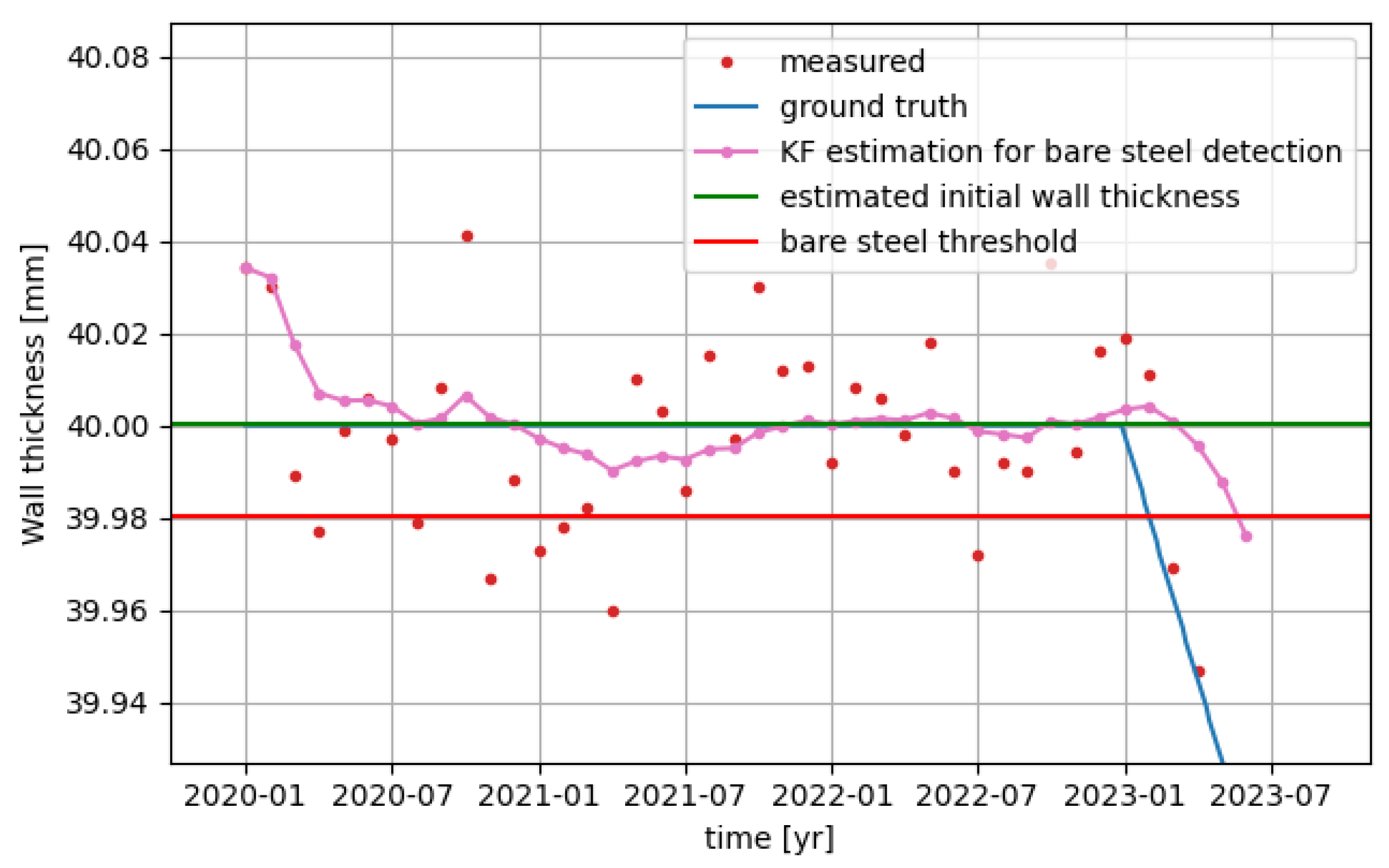
3.1. Corrosion Detection

This section describes a natural method for the detection of the onset of corrosion based on Bayesian filtering, which occurs when the protective coating has fully degraded and the bare steel becomes exposed.

The method to detect the onset of corrosion uses a constant (i.e., no-change) state-transition function F, which corresponds to the assumption that the coating is intact, i.e., no wall thickness degradation. In this case, F is a linear transformation (it is represented by an identity matrix) and, assuming a normally distributed process noise, Kalman filtering is a suitable algorithm for the estimation of the current wall thickness. Mathematically, a system state is a vector of dimension one consisting of the wall thickness. Interpreting such a vector as a scalar, we have $F=H=1$ ($H=1$ since we measure the wall thickness directly), and we have, cf. Section 2.1,

$$x_i:=(1-K_i)·x_{i-1}+K_i·z_i$$

(6)

$$p_i:=(1-K_i)·p_i^{\prime },$$

(7)

where

$$p_i^{\prime }:=p_{i-1}+q$$

(8)

$$K_i:=1/(1+r/p_i^{\prime })$$

(9)

and all terms are scalars (using lower case variable names to signify this). Notice that the distances of the value of $x_i$ to the previous estimate $x_{i-1}$ and to the measurement value $z_i$ are clearly determined by the Kalman gain $K_i\in [0,1]$.

The high-level idea of the algorithm is that corrosion onset is detected once the current wall thickness is significantly below the initial wall thickness, where the significance is defined by a fixed threshold value below the initial wall thickness. Due to manufacturing tolerances, the initial wall thickness is known only up to these some tolerances, and is likely more accurately estimated using ultrasound wall thickness measurements of the first few months (say, the first 6 months) assuming the coating has not yet been fully degraded during this time. In other words, the estimated initial wall thickness is, by definition, the estimated wall thickness after this fixed “calibration” time period. Note that the importance of an accurate estimation of the initial wall thickness. Indeed, if the assumed initial wall thickness is significantly higher than the actual wall thickness, then we erroneously detect corrosion onset straight away (a false positive). On the other hand, with an assumed initial wall thickness that is significantly lower than the actual wall thickness, the onset of corrosion will be detected too late (a false negative).

This calibration time period is a meta-parameter and must be chosen sufficiently short such that it is highly unlikely that the coating was fully degraded and sufficiently long that a reliable estimate can be obtained. Similarly, the threshold value is a meta-parameter of the algorithm. Suitable values for the calibration time and the detection threshold in general depend on the sample rate and measurement noise.

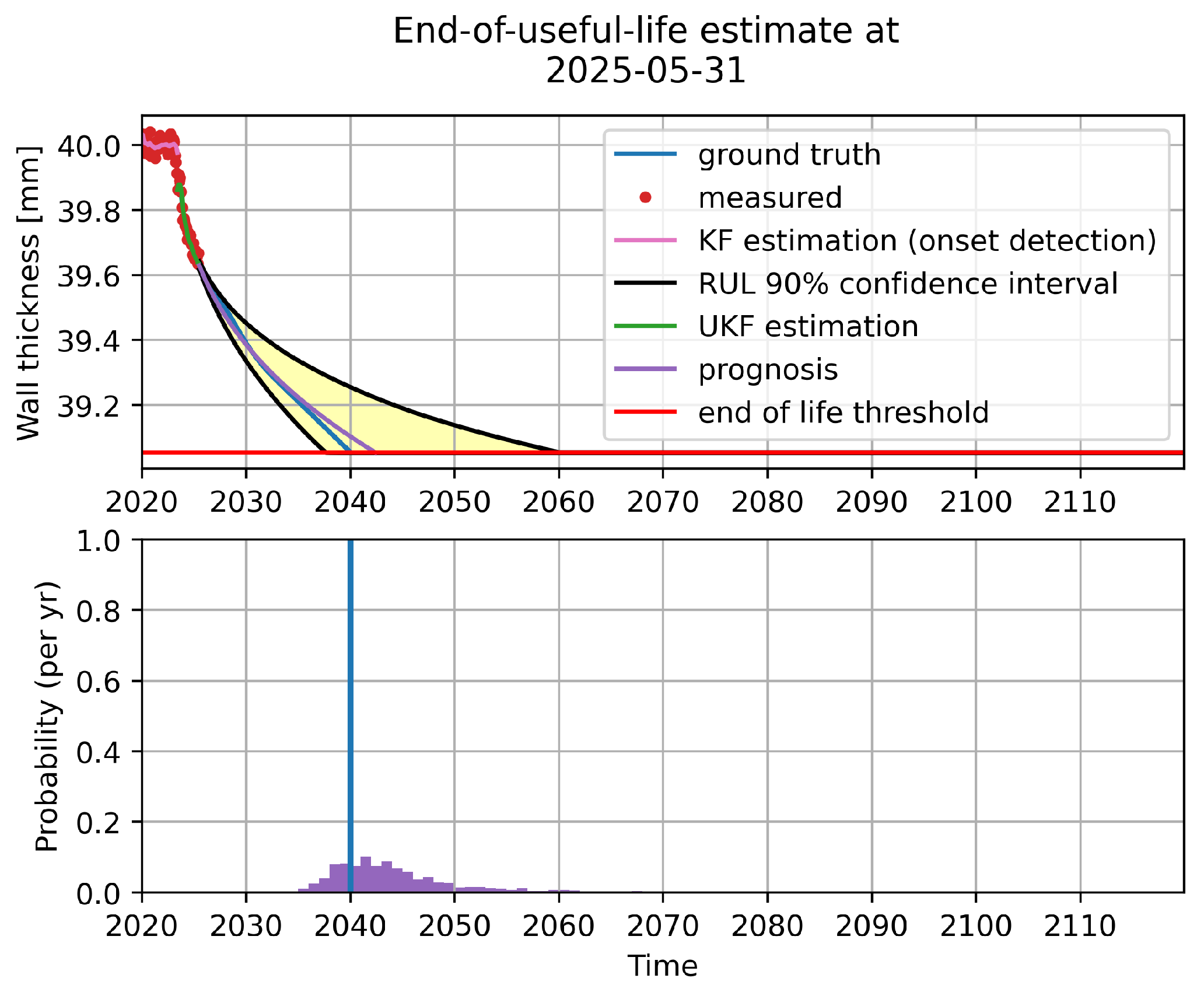
3.2. Corrosion Prognosis

3.2.1. Prognosis Algorithms

Prognosis of End-Of-Life (EOL) of offshore wind turbine structures is vital for scheduling maintenance, while avoiding system faults and escalation of damage. Prognosis can be based on historical data, e.g., the mean lifetime of an offshore wind turbine structure, or on online measurements, or both. In many application domains, the use of online measurements significantly improves prognostic performance compared to only using historical data. The prognosis method consists of two phases. In the first phase of the lifetime of a wind turbine structure, no corrosion has yet been detected and the EOL for the given location is assigned with a nominal probability distribution corresponding, for instance, to prior information on the duration of coating allowance within the applicable operating context. The second phase starts as soon as corrosion is detected. Once corrosion is detected we “switch” to one of the three above-described (ordinary or unscented) Kalman filtering approaches for estimation of the wall thickness during corrosion. This is an instance of a general paradigm called switching Kalman filtering, where different phases are treated by different Kalman filtering algorithms. In order to perform prognosis, the current estimate of the internal state $x_i$ is extrapolated by applying the state-transition function F iteratively.

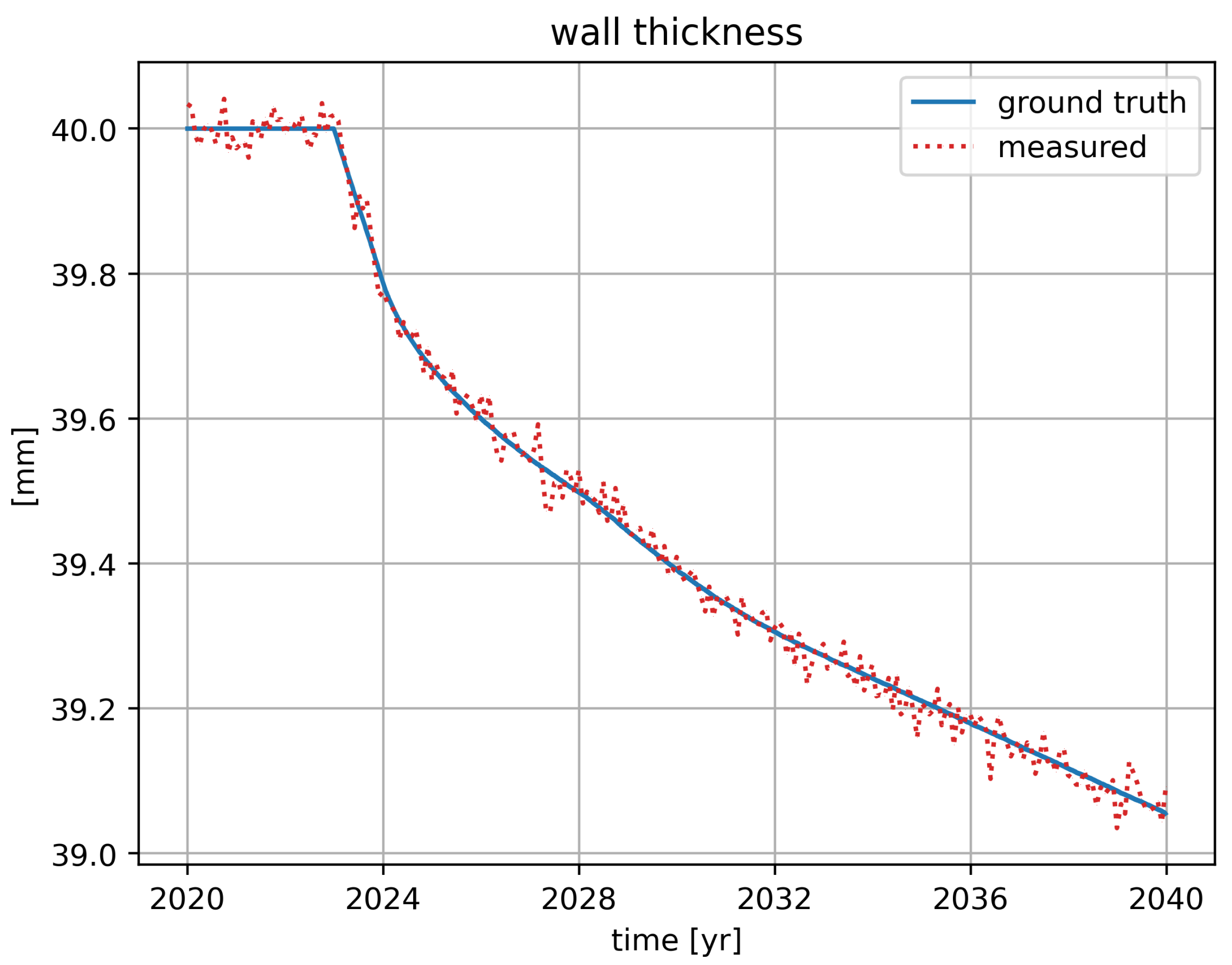
3.2.2. Wall Thickness Estimation during Steel Corrosion

An essential part of prognosis is the estimation of the wall thickness during steel corrosion. We consider three algorithms corresponding to three corrosion/degradation models in the literature:

• Linear corrosion model;
• Power-law corrosion model;
• Bi-modal corrosion model.

Each of these models assumes bare steel, and so these models are only used after corrosion is detected (i.e., when the steel is exposed due to coating degradation).

In general, a corrosion model $w\left(t\right)$ is a function describing wall thickness degradation over time due to corrosion. We have $w\left(t\right)=w_0-c_{\mathrm{loss}}\left(t\right)$, where $w_0$ denotes the initial wall thickness (e.g., in mm) and $c_{\mathrm{loss}}\left(t\right)$ denotes the loss of wall thickness after time t.

The linear corrosion model simply assumes a constant corrosion rate r, and so the corrosion loss is $c_{\mathrm{loss}}\left(t\right)=r·t$ and we have

$$w\left(t\right)=w_0-r·t.$$

(10)

For the Pourbaix equation [20] (see also [21]), we have $c_{\mathrm{loss}}\left(t\right)=A·t^p$, where A and p, with $0<p<1$, denote empirical constants assuming constant environmental conditions. Notice that the corrosion rate $A·p·t^{p-1}$ within this model is infinite initially (i.e., at $t=0$). A natural adaption is to introduce flexibility in the initial corrosion rate by introducing a non-negative time offset parameter $t_0$, to obtain $c_{\mathrm{loss}}\left(t\right)=A·{(t+t_0)}^p$ and so

$$w\left(t\right)=w_0-A·{(t+t_0)}^p.$$

(11)

By power-law corrosion model we denote this corrosion model adapted from the Pourbaix equation.

A refinement of the power-law corrosion model for time scales of decades is called the bi-modal corrosion model, proposed in [16]. This model has two “modes” where the corrosion rate in each mode decreases over time following the power-law corrosion model. Both modes also contain a constant corrosion rate phase: the power law is prepended by a constant corrosion rate phase in the first mode and appended by such a phase in the second mode. The first mode starts with a constant corrosion-rate phase, with a smooth transition to the power law model, while the second mode ends with a constant corrosion-rate phase. More precisely, the bi-modal model is defined in terms of corrosion rate as follows:

$$\begin{array}{c}\hfill \mathrm{biModalCorrRate}\left(t\right):=\left\{\begin{array}{cc}{A}_1·p_1·{t_1}^{p_1-1}\hfill & \mathrm{if}t\le t_s\hfill \\ A_1·p_1·{(t-t_s+t_1)}^{p_1-1}\hfill & \mathrm{if}{t}_s\le t\le t_{\mathrm{bi}}\hfill \\ A_2·p_2·{(t-t_{\mathrm{bi}}+t_2)}^{p_2-1}\hfill & \mathrm{if}{t}_{\mathrm{bi}}<t\le t_e\hfill \\ A_2·p_2·{(t_e-t_{\mathrm{bi}}+t_2)}^{p_2-1}\hfill & \mathrm{if}{t}_e\le t\hfill \end{array}\right.,\end{array}$$

(12)

where $A_i$ and $p_i$ are as in Equation (11) for each Mode $i\in \{1,2\}$, $t_s$ is the time of the start of the first power-law phase (and duration of the first phase), $t_{\mathrm{bi}}$ is the time of the start of Mode 2, and $t_e$ is the time of the second phase of Mode 2 (i.e., the start of the final linear phase). The values for $t_i$ are such that $r_{0,i}:=A_i·p_i·{t_i}^{p_i-1}$ correspond to the initial corrosion rates of each mode. Equivalently, we have

$$\begin{array}{c}\hfill \mathrm{biModalCorrRate}\left(t\right)=\left\{\begin{array}{cc}{r}_{0,1}\hfill & \mathrm{if}t\le t_{\mathrm{s}}\hfill \\ r_{0,1}·{((t-t_{\mathrm{s}})/t_1+1)}^{p_1-1}\hfill & \mathrm{if}{t}_{\mathrm{s}}\le t\le t_{\mathrm{bi}}\hfill \\ r_{0,2}·{((t-t_{\mathrm{bi}})/t_2+1)}^{p_2-1}\hfill & \mathrm{if}{t}_{\mathrm{bi}}<t\le t_{\mathrm{e}}\hfill \\ r_{0,2}·{((t_{\mathrm{e}}-t_{\mathrm{bi}})/t_2+1)}^{p_2-1}\hfill & \mathrm{if}{t}_{\mathrm{e}}\le t\hfill \end{array}\right..\end{array}$$

(13)

3.2.3. Implementation

Since the linear corrosion model corresponds to a linear state-transition function F, we use Kalman filtering for wall-thickness estimation. The other two corrosion models correspond to non-linear state-transitions functions, and so we use Unscented Kalman Filtering (UKF).

Linear Corrosion Model

We now consider a degradation model F based on constant-rate corrosion. In other words, we assume that the corrosion loss per unit of time is constant. Of course, constant-rate corrosion is a very crude approximation of the real corrosion process as, for example, it ignores external influences, such as temperature. Nevertheless, such a baseline algorithm might still give satisfying results, since, even though the degradation model assumes constant corrosion rate, the corrosion rate is constantly updated by Bayesian filtering (in fact, Kalman filtering) according to real-time incoming measurements.

Let us define a system state $x={\left(wr\right)}^T$ to be a column vector of length 2 consisting of the (estimated) wall thickness w and the (estimated) corrosion rate r. Recall that the model F sends each possible system state x to the next system state $x^{\prime }$ after some (fixed) period of time $\Delta t$. Therefore, $F\left(x\right)=x^{\prime }$ with $x^{\prime }={\left(w^{\prime }{r}^{\prime }\right)}^T$, $w^{\prime }=w-\Delta t·r$, and $r^{\prime }=r$. Indeed, since the corrosion rate r is fixed, $r^{\prime }=r$, and $w^{\prime }$ is simply the linear extrapolation of w corresponding to an increase in time $\Delta t$. We notice that F is a linear transformation (since $\Delta t$ is fixed), and so it is represented by the following matrix (which by slight abuse of notation we also denote by F):

$$F=\left[\begin{array}{cc}1& -\Delta t\\ 0& 1\end{array}\right].$$

(14)

Since we assume we measure the wall thickness directly (albeit with measurement noise), H simply sends x to the 1-by-1 matrix containing w. Therefore, H is the linear transformation represented by the matrix $H=\left[10\right]$.

To finalize the Kalman filter implementation of this corrosion model, we are left with defining the initial state $x_0$, the initial covariance matrix $P_0$, and the covariance matrices Q and R representing the magnitude of the process noise and the measurement noise. We assume the initial independence of the stochastic random variables w and r, and so $P_0$ is a diagonal matrix. Since the corrosion detection algorithm provides an estimate of the initial wall thickness $w_0$, we set the first entry of $x_0$ to this estimate. Moreover, we set the entry ${\left(P_0\right)}_{1,1}$ to the value of the 1-by-1 matrix P from the corrosion detection algorithm at the moment the corrosion detection algorithm fixes its initial wall thickness estimate. Since the initial corrosion rate is unknown, we set the second entry of $x_0$ to some “typical” value (we have chosen $0.2$) and set ${\left(P_0\right)}_{2,2}$ to a relatively large value of $0.{05}^2$. The 1-by-1 matrix R contains the variance ${\sigma }_R^2$ of the noise of the measurement device. The measurement noise level of ultrasound sensors is usually known and provided. For validation, we have considered several measurement noise levels ${\sigma }_R\in \{0.005,0.020,0.105\}$ consistent with noise levels encountered for ultrasound sensors. Since the model is a constant velocity model (the velocity being the corrosion rate), we use a process noise covariance matrix Q suitable for this type of model, as described in [22]. Specifically, $Q={\sigma }_Q^2·G^T·G$, where G is the row vector $\left(\frac{{(\Delta t)}^2}{2}\Delta t\right)$ and ${\sigma }_Q$ is a scalar. The value ${\sigma }_Q$ is difficult to estimate in practice, and is, therefore, often used as a “tuning” parameter. To automate tuning, we choose the value of ${\sigma }_Q$ that obtains highest accuracy for equidistant values on a base-10 log scale against some synthetic training datasets (see Section 4 for descriptions of the datasets and the accuracy metric). In this way, we have obtained ${\sigma }_Q=0.01$.

While, as mentioned above, there is a potentially large deviation of the ground truth with the constant-rate corrosion model, corresponding, therefore, to a relatively large process noise, it does enjoy a number of favorable properties compared to more complex models. First, F is linear, which together with linearity of H (and assuming normally distributed noise sources), allow for Kalman filtering to be applicable. Second, the length of the system state (it is of dimension 2) is essentially minimal, avoiding potential overfitting in state estimations relying on larger system states (as is the case of more complex models) and minimizes the problem of providing suitable initial estimates and (co)variances of unknown constants of the model (as only the initial estimate of the corrosion rate is required). Third, it provides robust results if the underlying physical mechanism is poorly understood (e.g., if certain external effects, such as temperature influence, are not known) or the measurement data are of (very) low quality. Fourth, since (1) the accuracy of corrosion prognosis for the remaining useful life estimation is most important near the end of life, and (2) as empirically confirmed in [16], the last phase of corrosion has a constant rate, we can expect accurate results in the most important last phase of the lifetime of an offshore wind turbine.

Bi-Modal and Power-Law Corrosion Models

Recall the bi-modal corrosion model of Equation (13) describing the corrosion rate as a function in time t. While several of the 9 parameters of this model are known to be temperature dependent [16], for Bayesian filtering we assume that they are constants. Similarly to as in the constant-rate corrosion model of Section 3.2.3, we rely on Bayesian filtering to adapt these constants to account for mechanisms and influences (such as temperature influences) not explicitly covered in the degradation model. If we would explicitly take into account, say, temperature influence, then this would result in a “blow-up” of constants that needs to be estimated. Indeed, in this case we would have, e.g., $t_{\mathrm{bi}}=a{e}^{bT}+c$ for some constants a, b, and c, resulting in a threefold increase in the number of constants to estimate (or fourfold if one includes the estimation of temperature itself).

Exactly as in Section 3.2.3, the wall thickness $w(t+\Delta t)$ at time $t+\Delta t$ is equal to $w\left(t\right)-\Delta t·\mathrm{corrRate}\left(t\right)$. A system state x is defined as an 11-tuple

$$(t,w,t_1,t_2,t_{\mathrm{s}},t_{\mathrm{bi}},t_{\mathrm{e}},r_{0,1},r_{0,2},p_1,p_2),$$

(15)

where t is the time, w is the wall thickness, and the other 9 values are the constants of Equation (13). We have $F\left(x\right)=x^{\prime }$, where ${\left(x^{\prime }\right)}_1=t+\Delta t$, ${\left(x^{\prime }\right)}_2=w-\Delta t·{\mathrm{corrRate}}_x\left(t\right)$ with ${\mathrm{corrRate}}_x\left(t\right)$ as in Equation (13) using the constants as given in x, and ${\left(x^{\prime }\right)}_i={\left(x\right)}_i$ for $i\in \{3,\dots ,11\}$. In other words, the values other than t and w are constants. The measurement function H simply sends x to its wall thickness entry ${\left(x\right)}_2$.

To finalize the unscented Kalman filter implementation of this corrosion model, we are again left with defining the initial state $x_0$ and the initial covariance matrices $P_0$, Q, and R. We set the entries of $x_0$ according to historical data provided in [16,23]. In particular, $p_1=0.5$, $p_2=1/3$, and at 20 ${}^{\circ }$C we have $r_{0,1}=r_{0,2}=0.2$, $t_1=0.23$, and $t_2=0.36$ (while adjustments can be made if the initial temperature is known, as described above, we take temperature into account through automatic adjustments due to Bayesian filtering). For matrix $P_0$ we assume the independence of the parameters (i.e., a diagonal matrix), where the entries corresponding to the constants $p_i$, $r_{0,i}$, and $t_i$ are set to a large uncertainty of ${\sigma }^2$ with $\sigma =0.1$. Again, we consider Q as a tuning matrix and automate the tuning. To avoid overfitting, we assume the process noise of the elements of the state are mutually independent, in other words, Q is a diagonal matrix. Moreover, optimize the accuracy of $Q:=s·P_0$ over a set of equidistant values for the scalar s in the base-10 log scale against the synthetic training datasets. Finally, matrix R is defined as in Section 3.2.3.

The power-law corrosion model is essentially a degenerate case of the bi-model corrosion model. A system state x is then defined as a 4-tuple

$$(t,w,A,p,t_0),$$

(16)

where the entries are as in Equation (11). Since the long-term behavior is most important, we mimic the power-law of the second mode in Equation (13) and choose $p=1/3$, $t_0=0.36$, and $A=r_{0,2}/\left(p·{t_0}^{p-1}\right)\approx 0.3$ (using, for the computation of A, the formula given in the paragraph above Equation (13)). Additionally, Q is computed in the same way as described for the bi-modal case.

Model Complexitity vs. State Estimation

The accuracy of a prognosis method is dependent on both the accuracy of the estimate of the current internal state and the accuracy of the degradation model. There is commonly a trade-off: the more accurate the degradation model, (typically) the more complex the degradation model (for example, more parameters to estimate), and so the more difficult it is to obtain an accurate estimate of the current internal state. The three degradation/corrosion models on which the three prognosis algorithms are based, reflect this trade-off: the bimodal corrosion model being the most accurate/complex model, the linear corrosion model being the simplest one, and the power law model in-between these two models regarding model complexity.

4. Results

In this section, we evaluate the performance of the corrosion detection algorithm and the three corrosion prognosis algorithms.

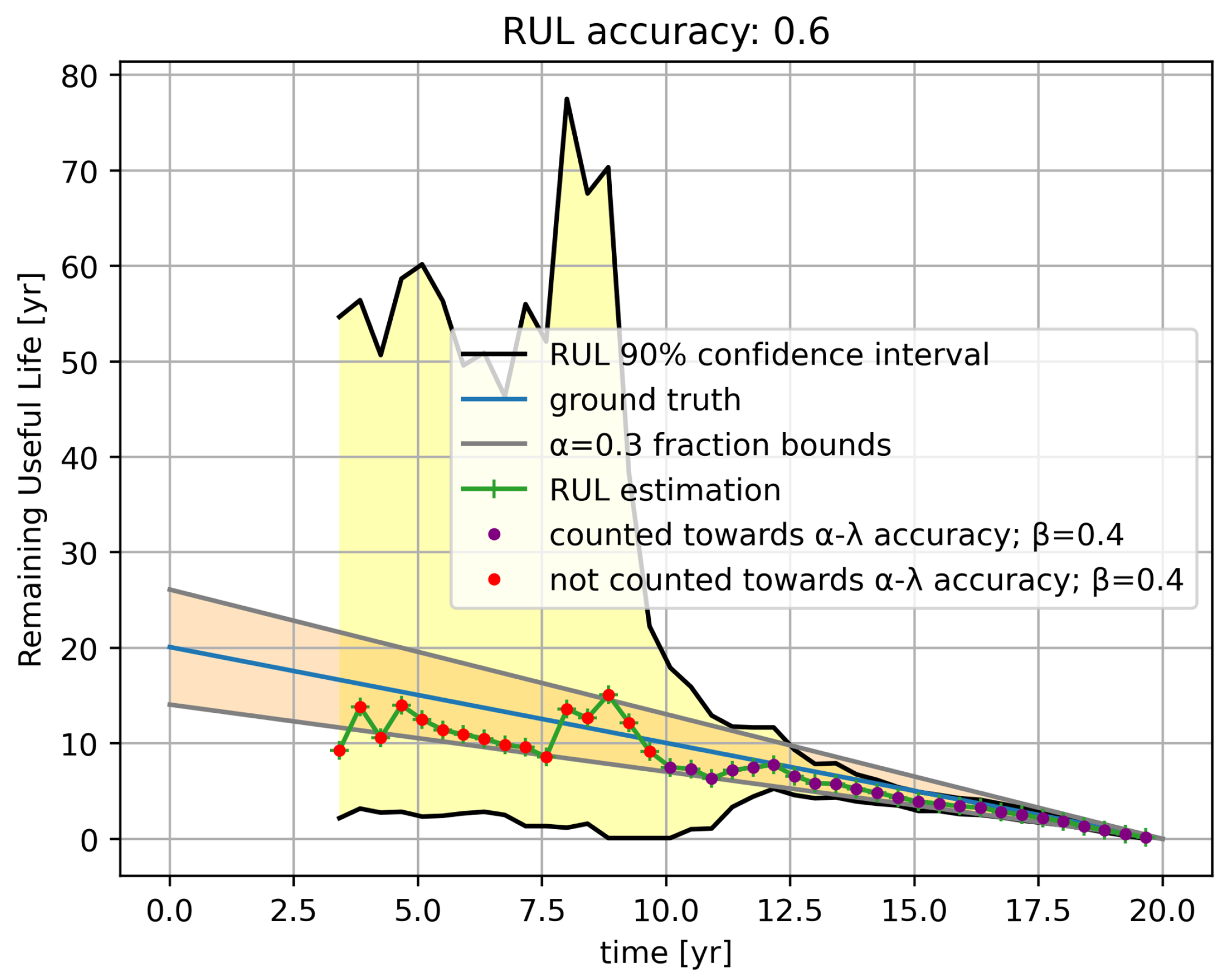
4.1. Performance Metric

To objectively compare the three prognosis algorithms, we employ the well-known $\alpha$-$\lambda$-accuracy metric [24]. This metric is defined as the fraction of the remaining useful life (RUL) estimations, from commencing the wind turbine until end of life, where at least an area of $\beta$ (with $\beta$ some value between 0 and 1) of the RUL distribution is within a factor of $1\pm \alpha$ of the ground truth RUL. Note that this accuracy metric is applied after EOL due to the required availability of the ground truth RUL.

4.2. Datasets

Due to limited available field data, we have simulated the wall thickness “ground truth” data and, using this ground truth data, also simulated the corresponding measurement data. The simulated ground truth data were obtained using the bimodal corrosion model. We assume here that the online monitoring system converts the raw ultrasound measurements into wall thickness values, which for convenience we simply call wall thickness measurements here. The parameters of the bi-modal model for which no suitable (real world) values were provided in [16], were instead estimated based on fitting (using a fitting tool that we specifically made for the bimodal corrosion model) the calculated corrosion-loss behavior from the corrosion loss plots given in that paper. In the bi-modal model, the corrosion rate at the end of the first mode is different from the corrosion rate at the beginning of the second mode leading to a discontinuity in the corrosion rate. Since such a discontinuity in corrosion rate is unrealistic, smoothing method is suggested. We employ the following smoothing method:

$$r_{\mathrm{transition}}\left(t\right)=w\left(t\right)r_1+(1-w\left(t\right))r_2,$$

(17)

where $r_{\mathrm{transition}}$ is the corrosion rate at time t with t between the start $t_{1,s}$ and end $t_{2,s}$ of the smoothing process, $r_1$ and $r_2$ are the corrosion rates for Mode 1 and Mode 2, respectively, assuming no smoothing, and

$$w\left(t\right)=\frac{t-t_{1,s}}{t_{2,s}-t_{1,s}}$$

(18)

is a weight factor. The temperature variation due to seasonal variation was simulated by a sine wave with a period of one year and an amplitude based on the seasonal temperature variation compatible with Canary islands as a concrete use case. Finally, we incorporated the influence of temperature on the level of corrosion by introducing a global factor of $e^{T-T_{\mathrm{ref}}}$ on the corrosion rate, as described in [23]. Various simulated ground truth corrosion datasets were generated using various realistic process and measurement noise variations and temperature variations. The ground truth is computed using a sampling rate of 0.01 year. From the simulated wall thickness ground truth, we have simulated corresponding wall thickness measurements by sampling at the expected measurement period of one month per position, and, following [11], a Gaussian measurement uncertainty was used with standard deviations ranging between 5 and 105 μm. An example simulated corrosion process with measurement data is given in Figure 1, where the coating has degraded after three years (i.e., the onset of corrosion starts in year 2023). Given the initial wall thickness, the three plots depicting the wall thickness, corrosion rate, and corrosion loss all represent the same information (assuming the initial wall thickness is known).

4.3. Corrosion Detection

Figure 2 shows the output of the corrosion detection algorithm on simulated measurement data from a single position of the wind turbine structure. This current wall thickness is the pink curve. The calibration time period is set to 8 months and the wall thickness detection threshold is set to 0.02 mm (recall these meta-parameters in Section 3.1).

Notice that several measurements that are coincidentally below the ground truth in the first half of 2021 do not lead to a detection, while corrosion is detected (the moment the pink curve drops below the red threshold line) 6 months after it commenced in the first month of 2023. This period of 6 months between corrosion onset and detection depends on the measurement noise and the measurement frequency, and can be reduced by increasing the measurement frequency.

4.4. Corrosion Prognosis

Figure 3 shows the output of the corrosion prognosis algorithm based on the power-law corrosion model on the above-described (simulated) measurement data (along with the ground truth for reference). The above-mentioned extrapolation of the current estimate of the internal state corresponds to the purple curve in the top plot of the figure. Recall that (ordinary or unscented) Kalman filtering provides more generally a probability distribution of the current estimate of the internal state. Extrapolating a large number of elements/particles drawn from this probability distribution allows one to obtain a confidence interval for prognosis (again top plot of the figure) and a probability distribution for the EOL estimate (bottom plot in the figure).

4.5. Accuracy of Remaining Useful Life Estimates

Figure 4 illustrates the computation of the $\alpha$-$\lambda$-accuracy metric on a dataset containing measurements from corrosion detection (after 3 years) until end of life. The red (purple, resp.) dots correspond to timestamps where less (more, resp.) than an area of $\beta$ of the RUL distribution is within a factor of $1\pm \alpha$ of the ground truth RUL. The fraction of purple dots among the purple and red dots is 0.6, and so the $\alpha$-$\lambda$-accuracy for this dataset is 0.6. To obtain a robust comparison of the three prognosis algorithms, we compare the mean of the $\alpha$-$\lambda$-accuracy values over five representative datasets with varying relevant measurement and process noise and temperature variations. The results are shown in

Table 1. Comparison of the accuracy of the prognosis algorithms based on the three corrosion models. Highest mean accuracy in bold.

Prognosis Algorithm	Mean Accuracy
Linear	0.400
Power law	0.415
Bimodal	0.376

. We observe that the prognosis algorithm based on the power law model performs best, and, therefore, this algorithm is selected as the final prognosis algorithm.

5. Conclusions

We considered a corrosion detection method and three corrosion prognosis methods based on Bayesian filtering, in particular, ordinary and unscented Kalman filtering. The three corrosion prognosis methods cover a range of corrosion model complexities, from the very simple linear corrosion model to the involved bimodal corrosion model, to evaluate the trade-off between model accuracy and current state estimation accuracy. Using the $\alpha$-$\lambda$-accuracy metric, we quantitatively compared the performance of the three prognosis algorithms against a number of synthetic datasets, which cover a range of measurement and process noise levels typical for wall thickness measurements of offshore wind turbines using ultrasound sensors. We observed that the prognosis method based on the power-law corrosion model (in model complexity between the linear corrosion model and the bimodal corrosion model) has the highest mean accuracy score.

References

1. Coronado, D.; Fischer, K. Condition Monitoring of Wind Turbines: State of the Art, User Experience and Recommendations; Technical Report; Fraunhofer Institute for Wind Energy and Energy System Technology (Fraunhofer IWES): Bremerhaven, Germany, 2015; Available online: https://www.vgb.org/vgbmultimedia/383_Final+report-p-9786.pdf (accessed on 5 October 2022).
2. Martinez-Luengo, M.; Kolios, A.; Wang, L. Structural health monitoring of offshore wind turbines: A review through the Statistical Pattern Recognition Paradigm. Renew. Sustain. Energy Rev. 2016, 64, 91–105. [Google Scholar] [CrossRef] [Green Version]
3. Adedipe, O.; Brennan, F.; Kolios, A. Review of corrosion fatigue in offshore structures: Present status and challenges in the offshore wind sector. Renew. Sustain. Energy Rev. 2016, 61, 141–154. [Google Scholar] [CrossRef]
4. Watereye Consortium. Watereye Project Website. 2022. Available online: https://watereye-project.eu/ (accessed on 5 October 2022).
5. Thibbotuwa, U.C.; Cortés, A.; Irizar, A. Ultrasound-Based Smart Corrosion Monitoring System for Offshore Wind Turbines. Appl. Sci. 2022, 12, 808. [Google Scholar] [CrossRef]
6. Verhelst, J.; Coudron, I.; Ompusunggu, A.P. SCADA-Compatible and Scaleable Visualization Tool for Corrosion Monitoring of Offshore Wind Turbine Structures. Appl. Sci. 2022, 12, 1762. [Google Scholar] [CrossRef]
7. Ahuir-Torres, J.I.; Bausch, N.; Farrar, A.; Webb, S.; Simandjuntak, S.; Nash, A.; Thomas, B.; Muna, J.; Jonsson, C.; Mathew, D. Benchmarking parameters for remote electrochemical corrosion detection and monitoring of offshore wind turbine structures. Wind. Energy 2019, 22, 857–876. [Google Scholar] [CrossRef] [Green Version]
8. Liu, Y.; Hajj, M.; Bao, Y. Review of robot-based damage assessment for offshore wind turbines. Renew. Sustain. Energy Rev. 2022, 158, 112187. [Google Scholar] [CrossRef]
9. Chookah, M.; Nuhi, M.; Modarres, M. A probabilistic physics-of-failure model for prognostic health management of structures subject to pitting and corrosion-fatigue. Reliab. Eng. Syst. Saf. 2011, 96, 1601–1610. [Google Scholar] [CrossRef]
10. Vachtsevanos, G. Corrosion Diagnostic and Prognostic Technologies. In Corrosion Processes: Sensing, Monitoring, Data Analytics, Prevention/Protection, Diagnosis/Prognosis and Maintenance Strategies; Vachtsevanos, G., Natarajan, K.A., Rajamani, R., Sandborn, P., Eds.; Springer: Cham, Switzerland, 2020; pp. 231–311. [Google Scholar] [CrossRef]
11. Rommetveit, T.; Johnsen, R.; Johansen, T.F.; Baltzersen, Ø. High Resolution Ultrasound Wall Thickness Measurements through Polyester Coating and Real-Time Process Control. In Proceedings of the Corrosion 2009, Atlanta, GA, USA, 22–26 March 2009; NACE International: San Diego, CA, USA, 2009. [Google Scholar]
12. Rommetveit, T.; Johansen, T.F.; Johnsen, R. A Combined Approach for High-Resolution Corrosion Monitoring and Temperature Compensation Using Ultrasound. IEEE Trans. Instrum. Meas. 2010, 59, 2843–2853. [Google Scholar] [CrossRef]
13. Vásquez, S.; Verhelst, J.; Brijder, R.; Ompusunggu, A. Corrosion Detection, Prognosis and Decision Support Tool for Offshore Wind Turbine Structures. Wind 2022, 2, 747–765. [Google Scholar] [CrossRef]
14. Särkkä, S. Bayesian Filtering and Smoothing; Institute of Mathematical Statistics (IMS) Textbooks; Cambridge University Press: Cambridge, UK, 2013. [Google Scholar] [CrossRef]
15. Brijder, R.; Hagen, C.H.M.; Cortés, A.; Irizar, A.; Thibbotuwa, U.C.; Helsen, S.; Vásquez, S.; Ompusunggu, A.P. Review of corrosion monitoring and prognostics in offshore wind turbine structures: Current status and feasible approaches. Front. Energy Res. 2022, 10, 991343. [Google Scholar] [CrossRef]
16. Melchers, R.E. Progress in developing realistic corrosion models. Struct. Infrastruct. Eng. 2018, 14, 843–853. [Google Scholar] [CrossRef]
17. Brijder, R.; Helsen, S.; Ompusunggu, A.P. Corrosion Prognostics for Offshore Wind-Turbine Structures using Bayesian Filtering with Bi-modal and Linear Degradation Models. In Proceedings of the 13th International Workshop on Structural Health Monitoring (IWSHM), Stanford, CA, USA, 15–17 March 2022; Farhangdoust, S., Guemes, A., Chang, F.K., Eds.; DEStech Publications, Inc.: Lancaster, PA, USA, 2022; pp. 452–459. [Google Scholar]
18. Kalman, R.E. A New Approach to Linear Filtering and Prediction Problems. J. Basic Eng. 1960, 82, 35–45. [Google Scholar] [CrossRef] [Green Version]
19. Wan, E.A.; Van Der Merwe, R. The unscented Kalman filter for nonlinear estimation. In Proceedings of the IEEE 2000 Adaptive Systems for Signal Processing, Communications, and Control Symposium, Lake Louise, AB, Canada, 1–4 October 2000; pp. 153–158. [Google Scholar]
20. Pourbaix, M. International cooperation in the prevention of corrosion of materials. In Proceedings of the IX International Congress of Metallic Corrosion, Toronto, ON, Canada, 3–7 June 1990; Volume 1, pp. 57–100. [Google Scholar]
21. Kenny, E.D.; Paredes, R.S.; de Lacerda, L.A.; Sica, Y.C.; de Souza, G.P.; Lázaris, J. Artificial neural network corrosion modeling for metals in an equatorial climate. Corros. Sci. 2009, 51, 2266–2278. [Google Scholar] [CrossRef]
22. Bar-Shalom, Y.; Li, X.; Kirubarajan, T. Estimation for Kinematic Models. In Estimation with Applications to Tracking and Navigation; John Wiley & Sons, Ltd.: Hoboken, NJ, USA, 2002; Chapter 6; pp. 267–299. [Google Scholar] [CrossRef]
23. Melchers, R. Maritime Corrosion—New insights. In Proceedings of the Symposion on Corrosion and Fouling, Warsaw, Poland, 2–7 June 2019; Available online: http://corrosion.hzs.be/abstracts.html#Melchers (accessed on 1 April 2021).
24. Saxena, A.; Celaya, J.; Saha, B.; Saha, S.; Goebel, K. Metrics for Offline Evaluation of Prognostic Performance. Int. J. Progn. Health Manag. 2010, 1, 1. [Google Scholar] [CrossRef]
Figure 1. A dataset of simulated wall thickness measurements (a Gaussian measurement noise with a standard deviation of 20 μm is used here) along with the ground truth and the corresponding corrosion rate and corrosion loss. Only the wall thickness measurements are used in the corrosion detection and corrosion prognosis [24].
Wind 03 00001 g001
Figure 2. Output of the corrosion detection algorithm on simulated measurement data of a single position, along with the ground truth for reference. Again, a Gaussian measurement noise with a standard deviation of 20 μm is used here.
Wind 03 00001 g002
Figure 3. Output of the corrosion prognosis algorithm based on the power-law corrosion model on (simulated) measurement data, along with the ground truth for reference, see also [13].
Wind 03 00001 g003
Figure 4. Remaining useful life estimates over time, along with the ground truth and an illustration of the computation of the corresponding α - λ -accuracy.
Wind 03 00001 g004