


Detection, Prognosis and Decision Support Tool for Offshore Wind Turbine Structures


Abstract
:1. Introduction
1.1. Main Contributions
1.2. Paper Organisation
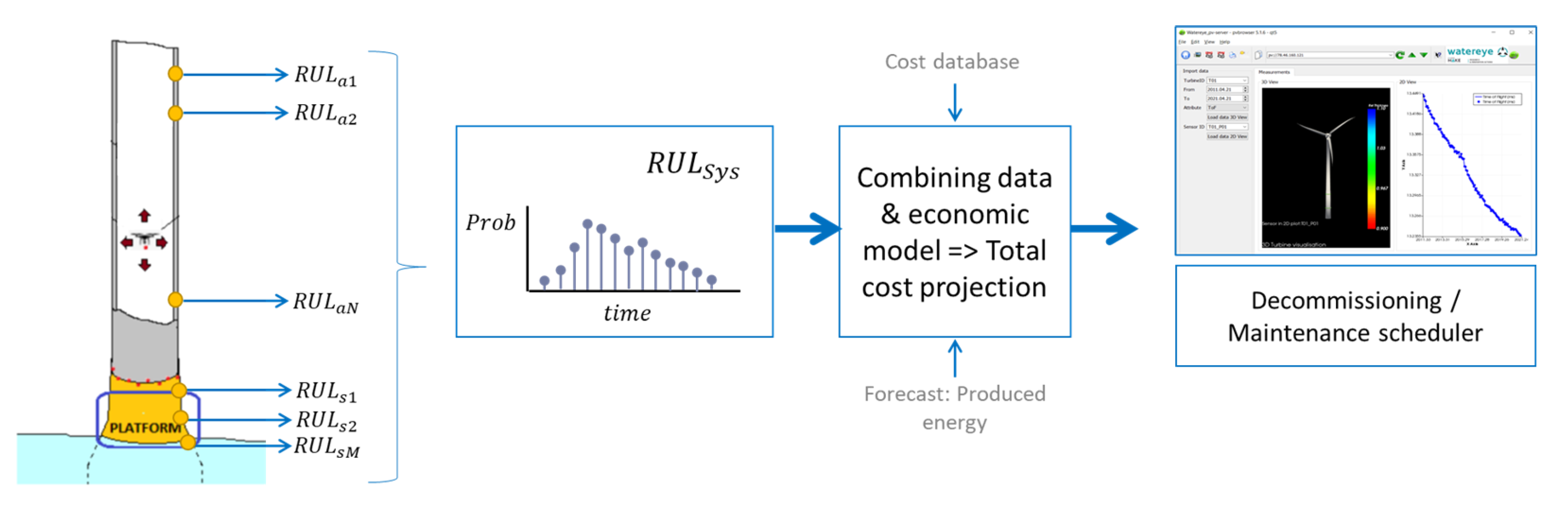
2. Overview of the Developed System
3. Corrosion Detection and Prognosis
3.1. Methodology
3.2. Local Detection and Prognosis
3.2.1. Corrosion Detection
3.2.2. Corrosion Prognosis
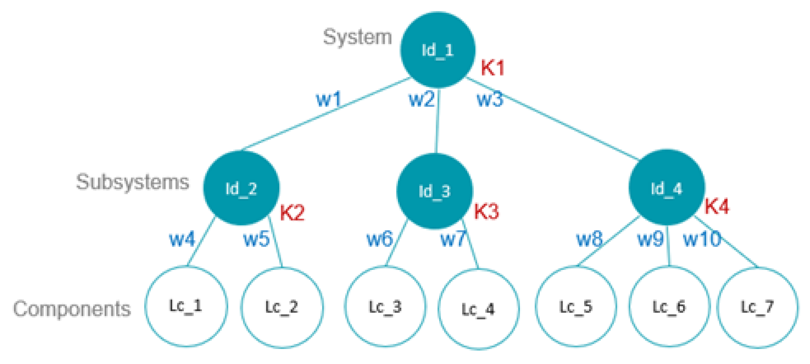
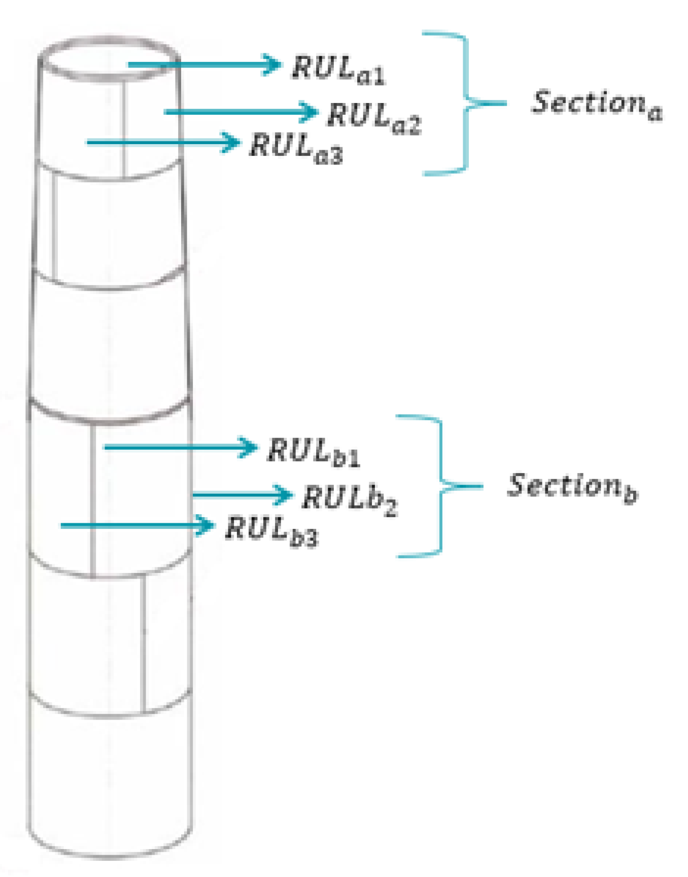
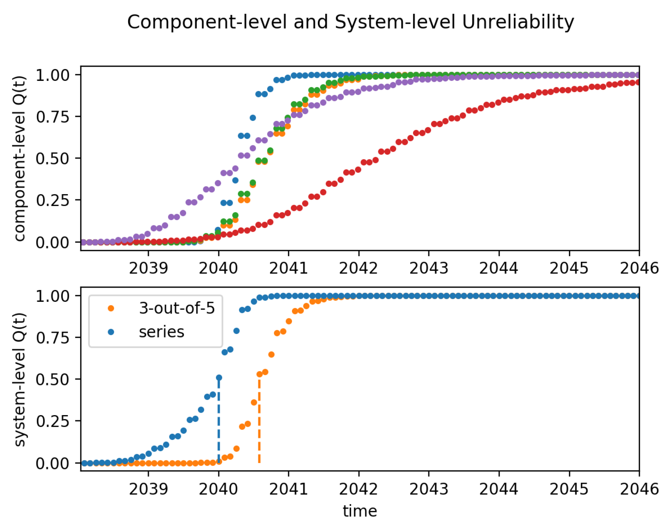
3.3. System-Level Prognosis
4. Decision Support Tool
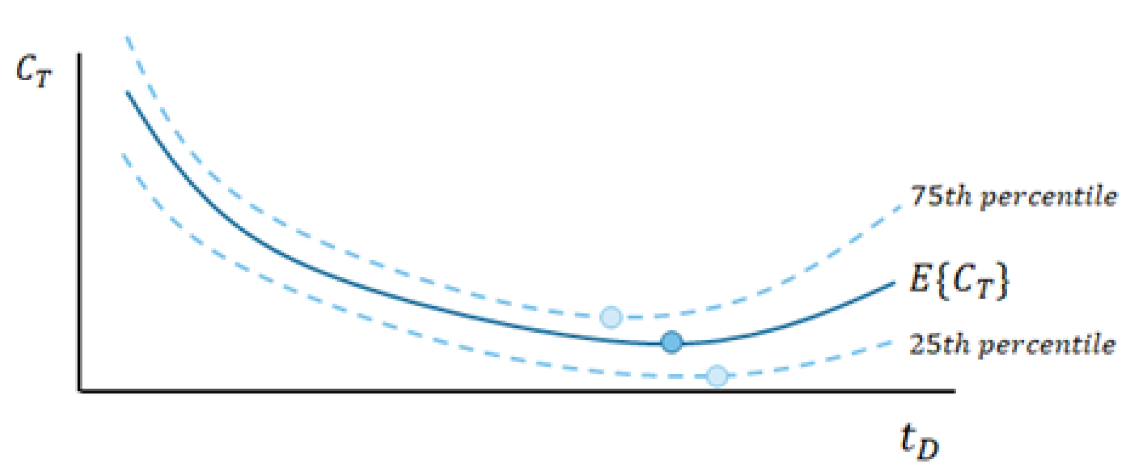
4.1. Economical Optimization
4.2. Definitions for Economical Optimization
- Capital costs ()This cost involves the wind turbine investment (i.e., all costs related to the initial investment for bringing the wind turbine to an operable status), including the investment for implementing the monitoring and prognosis software and hardwareThese costs may be considered as a single payment or spread in time following an amortization formula, taking into account loan interest rates. Note that is a fixed cost that does not depend on or , and so it does not contribute to the optimization of . However, it does serve for the interpretation of the results.
- Operational costs ()This cost term encompasses all ongoing expenses that are inherent to the operation of the wind turbine (such as operation, maintenance, inspection, insurance, leasing and taxes costs). With regard to the impact of the failure, we split this cost aswhere is a monthly recurring cost that continues until the decommissioning or failure date, defined as:where reflects the costs before the failure, and —the incurring costs of preserving the asset, once the failure takes place, until the decommissioning (e.g., additional inspections). is a one-time-incurred cost that lumps all costs related with the failure. It is defined aswithNotably, the use of the delta Dirac function reflects the fact that if the decommissioning takes place before the failure, there are no costs associated to it. The cost includes both direct and indirect losses due to the failure occurrence. Direct losses include, for instance, fines due to inoperability of the asset and inspections or corrective actions that need to take place because of the failure. Indirect losses include environmental, human, and financial losses. Note that the production losses are included as part of , which is defined below.
- Decommissioning costs ()This one-time cost summarizes all costs related to the decommissioning of the wind turbine.with denoting the cost of decommission being defined as:which reflects the possible difference in costs depending on the occurrence of the failure (i.e., ). Note that the time dependency of these costs allows for penalizing actions that take place during months where the accessibility to the wind turbine is difficult due to, for example, weather conditions or logistics.
- Produced energy ()The produced energy is defined as:with denoting the expected produced energy in a failure-free condition (e.g., estimated from historical production data or from a wind resource characterization of the site including the expected turbine efficiency and possibly the reduction of production due to wake effects), and denoting a function that reflects the impact of the failure and the decommissioning being defined as:
- Income for produced energy ()This income is defined as:with denoting the price of energy per unit.Note that the remaining value of the asset after decommissioning is not included explicitly as a separate income term, as it is not recurrent, it is highly uncertain and difficult to estimate years in advance. However, it can be included indirectly by the users of the methodology, by merging this remaining value as an income term (thus, a negative modifier) to the decommissioning term .
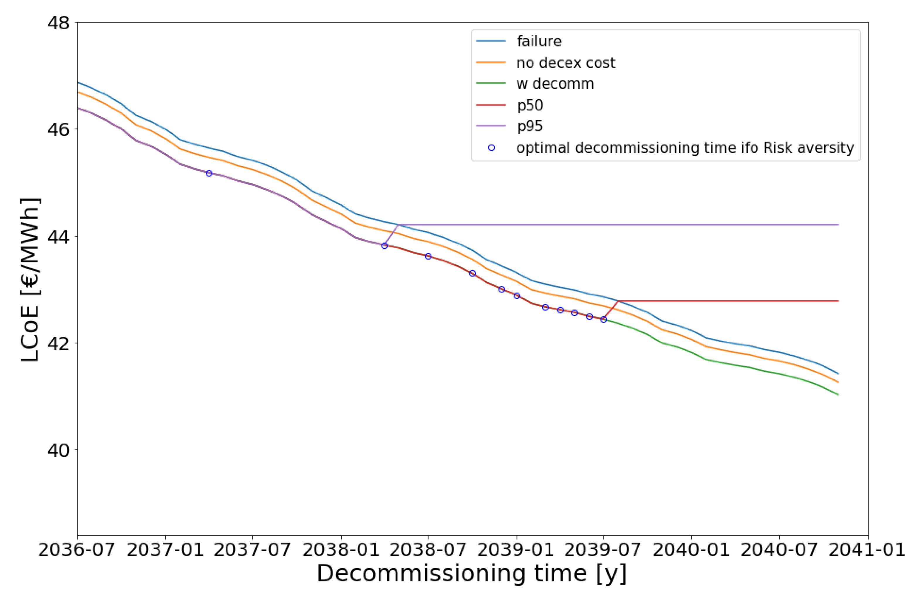
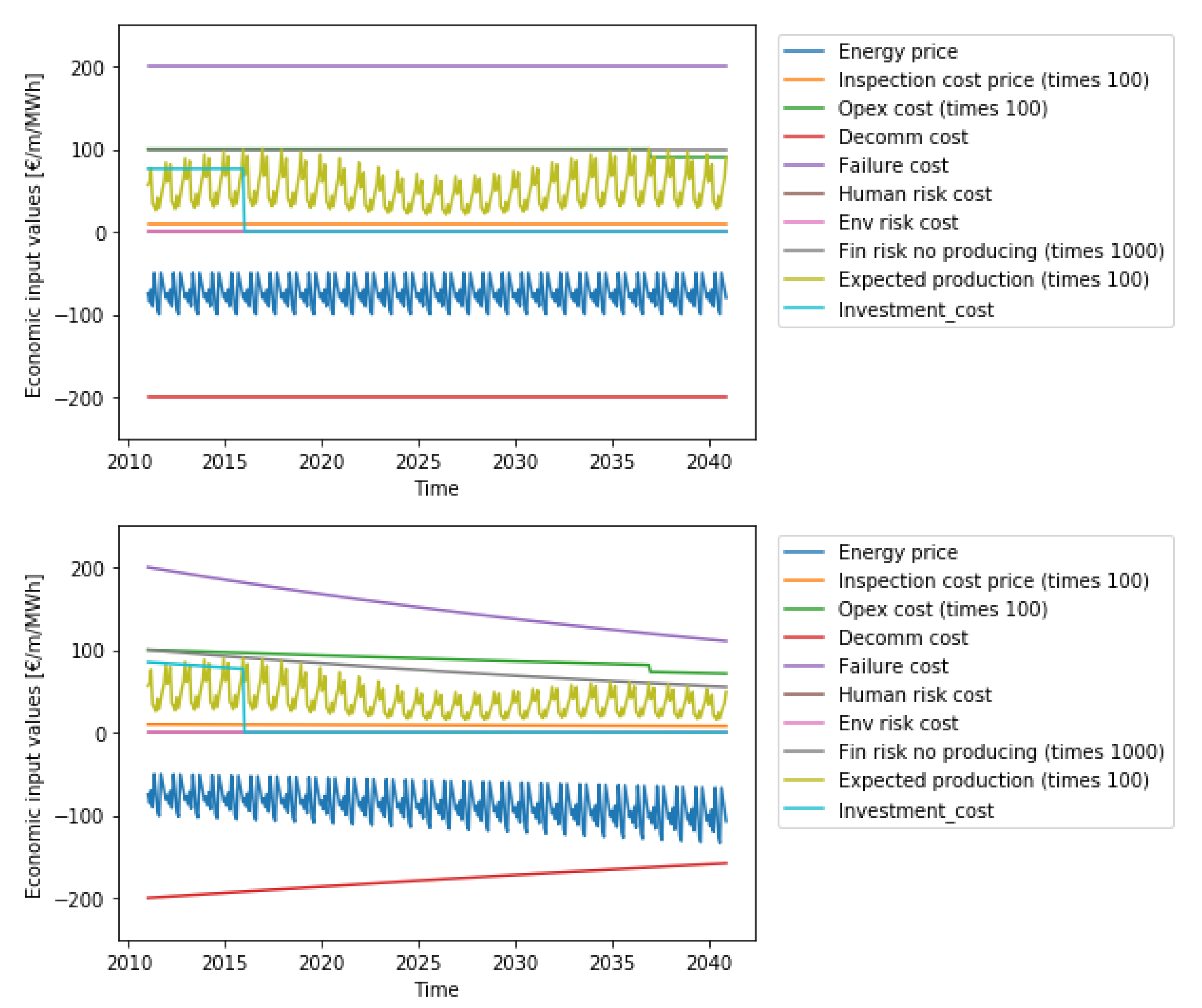
4.3. Simulation
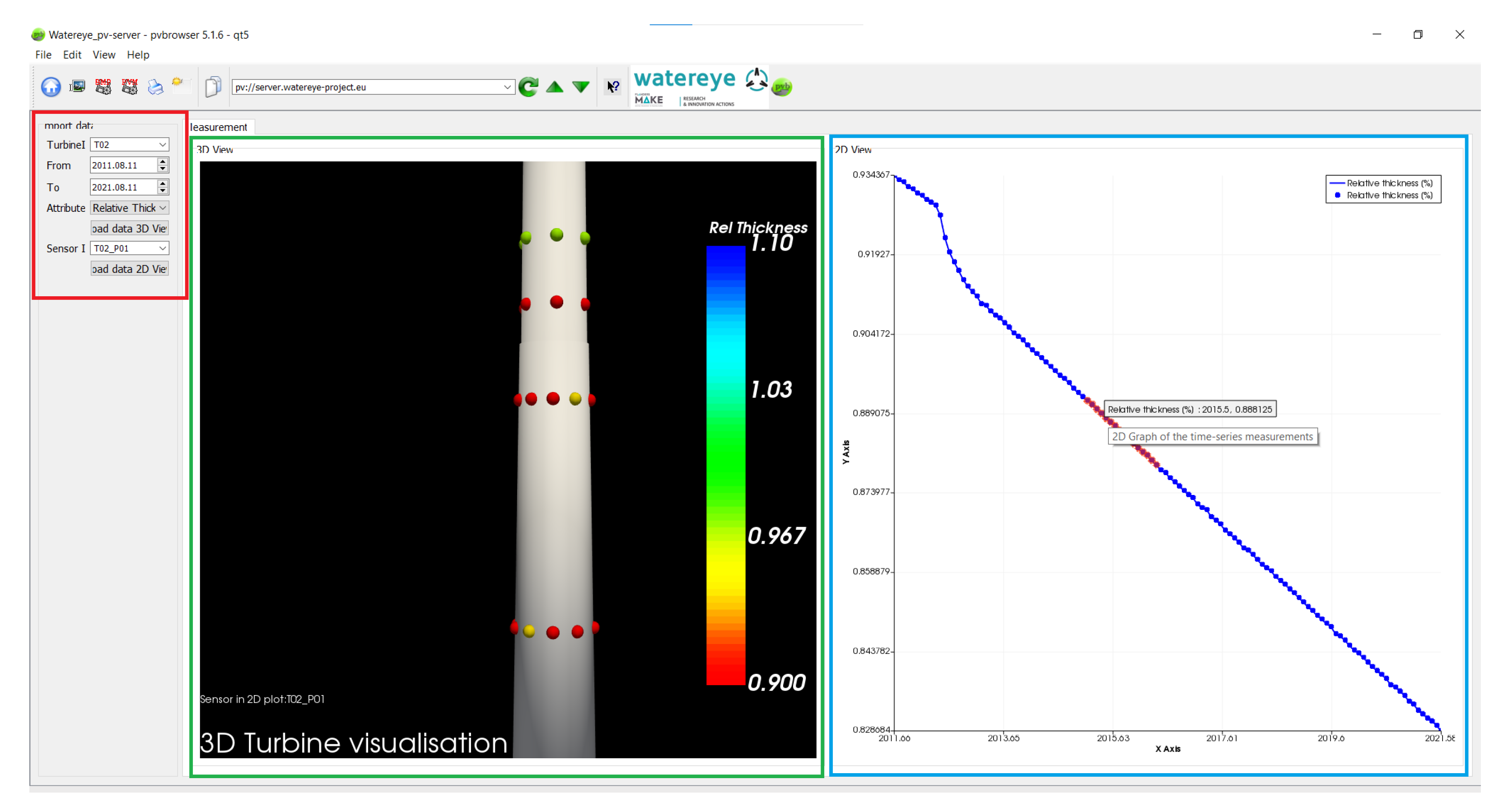
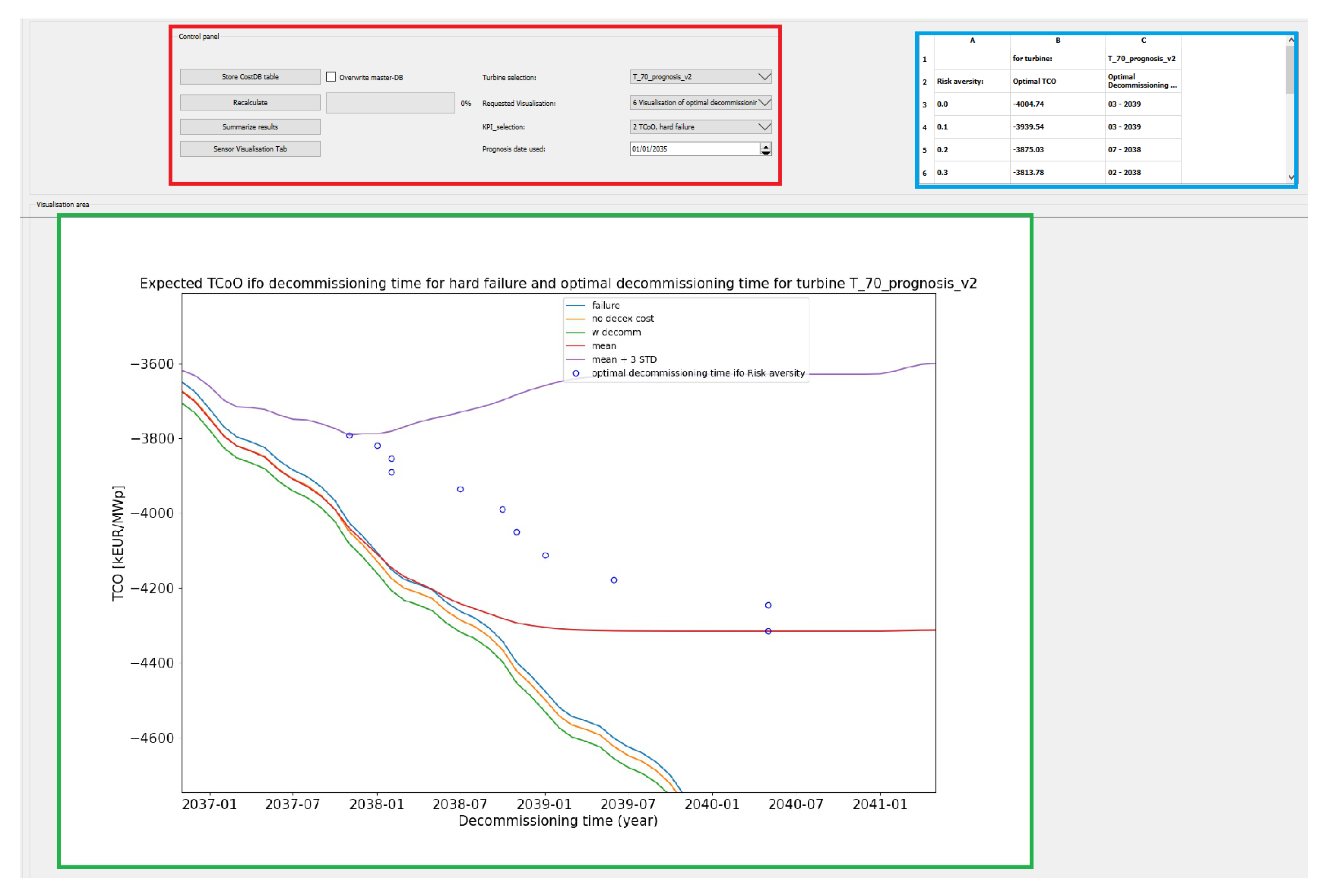
5. Graphical User Interface
6. Conclusions
Author Contributions
Funding
Institutional Review Board Statement
Informed Consent Statement
Data Availability Statement
Acknowledgments
Conflicts of Interest
Appendix A. Economic Assumptions

References
- Global Wind Energy Council (GWEC). GWEC Global Wind Report 2022; GWEC: Brussels, Belgium, 2022. [Google Scholar]
- International Renewable Energy Agency (IRENA). Renewable Power Generation Costs in 2019; IRENA: Abu Dhabi, United Arab Emirates, 2020. [Google Scholar]
- Chen, J.; Kim, M.H. Review of Recent Offshore Wind Turbine Research and Optimization Methodologies in Their Design. J. Mar. Sci. Eng. 2022, 10, 28. [Google Scholar] [CrossRef]
- Failla, G.; Arena, F. New perspectives in offshore wind energy. Philos. Top. 2015, 373, 20140228. [Google Scholar] [CrossRef] [PubMed] [Green Version]
- Wu, X.; Hu, Y.; Li, Y.; Yang, J.; Duan, L.; Wang, T.; Adcock, T.; Jiang, Z.; Gao, Z.; Lin, Z.; et al. Foundations of offshore wind turbines: A review. Renew. Sustain. Energy Rev. 2019, 104, 379–393. [Google Scholar] [CrossRef] [Green Version]
- Price, S.J.; Figueira, R.B. Corrosion Protection Systems and Fatigue Corrosion in Offshore Wind Structures: Current Status and Future Perspectives. Coatings 2017, 7, 25. [Google Scholar] [CrossRef]
- Martinez-Luengo, M.; Kolios, A.; Wang, L. Structural health monitoring of offshore wind turbines: A review through the Statistical Pattern Recognition Paradigm. Renew. Sustain. Energy Rev. 2016, 64, 91–105. [Google Scholar] [CrossRef] [Green Version]
- Brijder, R.; Hagen, C.H.M.; Cortés, A.; Irizar, A.; Thibbotuwa, U.C.; Helsen, S.; Vásquez, S.; Ompusunggu, A.P. Review of corrosion monitoring and prognostics in offshore wind turbine structures: Current status and feasible approaches. Front. Energy Res. 2022, 10, 1433. [Google Scholar] [CrossRef]
- Verhelst, J.; Coudron, I.; Ompusunggu, A.P. SCADA-Compatible and Scaleable Visualization Tool for Corrosion Monitoring of Offshore Wind Turbine Structures. Appl. Sci. 2022, 12, 1762. [Google Scholar] [CrossRef]
- WATEREYE_H2020. O&M Tools Integrating Accurate Structural Health in Offshore Energy. 2022. Available online: https://cordis.europa.eu/project/id/851207 (accessed on 7 September 2022).
- Thibbotuwa, U.C.; Cortés, A.; Irizar, A. Ultrasound-Based Smart Corrosion Monitoring System for Offshore Wind Turbines. Appl. Sci. 2022, 12, 808. [Google Scholar] [CrossRef]
- Ortegon, K.; Nies, L.F.; Sutherland, J.W. Preparing for end of service life of wind turbines. J. Clean. Prod. 2013, 39, 191–199. [Google Scholar] [CrossRef]
- Topham, E.; Gonzalez, E.; McMillan, D.; João, E. Challenges of decommissioning offshore wind farms: Overview of the European experience. In Proceedings of the WindEurope Conference and Exhibition 2019, Journal of Physics: Conference Series, Bilbao, Spain, 2–4 April 2019; Volume 1222. [Google Scholar]
- Irawan, C.A.; Wall, G.; Jones, D. An optimisation model for scheduling the decommissioning of an offshore wind farm. OR Spectrum 2019, 41, 513–548. [Google Scholar] [CrossRef]
- DNV GL AS. DNVGL-RP-0416: Corrosion Protection for Wind Turbines; Technical Report; DNV GL AS: Høvik, Norway, 2016. [Google Scholar]
- DNV GL AS. DNVGL-ST-0126: Support Structures for Wind Turbines. Technical Report; DNV GL AS: Høvik, Norway, 2016. [Google Scholar]
- Daigle, M.; Bregon, A.; Roychoudhury, I. A Distributed Approach to System-Level Prognostics. In Proceedings of the Annual Conference of the PHM Society, Minneapolis, MN, USA, 23–27 September 2012; Volume 4. [Google Scholar] [CrossRef]
- Brijder, R.; Helsen, S.; Ompusunggu, A.P. Switching Kalman Filtering Based Corrosion Detection and Prognostics for Offshore Wind-Turbine Structures. Wind, 2022; Submitted. [Google Scholar]
- Pourbaix, M. International cooperation in the prevention of corrosion of materials. In Proceedings of the IX International Congress of Metallic Corrosion, Toronto, ON, Canada, 3–7 June 1984; Volume 1, pp. 57–100. [Google Scholar]
- Kalman, R.E. A New Approach to Linear Filtering and Prediction Problems. J. Basic Eng. 1960, 82, 35–45. [Google Scholar] [CrossRef] [Green Version]
- Brijder, R.; Helsen, S.; Ompusunggu, A.P. Corrosion Prognostics for Offshore Wind-Turbine Structures using Bayesian Filtering with Bi-modal and Linear Degradation Models. In Proceedings of the 13th International Workshop on Structural Health Monitoring (IWSHM 2021), Stanford, CA, USA, 15–17 March 2022. [Google Scholar]
- Melchers, R.E. Progress in developing realistic corrosion models. Struct. Infrastruct. Eng. 2018, 14, 843–853. [Google Scholar] [CrossRef]
- Wu, J.S.; Chen, R.J. An algorithm for computing the reliability of weighted-k-out-of-n systems. IEEE Trans. Reliab. 1994, 43, 327–328. [Google Scholar] [CrossRef] [Green Version]
- Chang, Y.; Mai, Y.; Yi, L.; Yu, L.; Chen, Y.; Yang, C.; Gao, J. Reliability Analysis of k-out-of-n Systems of Components with Potentially Brittle Behavior by Universal Generating Function and Linear Programming. Math. Probl. Eng. 2020, 2020, 8087242. [Google Scholar] [CrossRef] [Green Version]
- Louhichi, R.; Sallak, M.; Pelletan, J. A cost model for predictive maintenance based on risk-assessment. In Proceedings of the 13ème Conférence Internationale CIGI QUALITA 2019, HAL, Montreal, QC, Canada, 14 August 2019. [Google Scholar]
- Jin, T.; Tian, Z.; Huerta, M.; Piechota, J. Coordinating maintenance with spares logistics to minimize levelized cost of wind energy. In Proceedings of the 2012 International Conference on Quality, Reliability, Risk, Maintenance, and Safety Engineering, Chengdu, China, 15–18 June 2012; pp. 1022–1027. [Google Scholar] [CrossRef]
- Feng, J.; Cai, H.; Liu, Z.; Lee, J. A Systematic Framework for Maintenance Scheduling and Routing for Off-Shore Wind Farms by Minimizing Predictive Production Loss. In Proceedings of the E3S Web of Conferences, 2020 2nd International Academic Exchange Conference on Science and Technology Innovation, Guangzhou, China, 18–20 December 2020. [Google Scholar] [CrossRef]
- Lei, X.; Sandborn, P.; Bakhshi, R.; Kashani-Pour, A.; Goudarzi, N. PHM based predictive maintenance optimization for offshore wind farms. In Proceedings of the 2015 IEEE Conference on Prognostics and Health Management (PHM), Austin, TX, USA, 22–25 June 2015; pp. 1–8. [Google Scholar] [CrossRef]
- Besnard, F.; Patriksson, M.; Strömberg, A.B.; Wojciechowski, A.; Bertling, L. An optimization framework for opportunistic maintenance of offshore wind power system. In Proceedings of the 2009 IEEE Bucharest PowerTech, Bucharest, Romania, 28 June–2 July 2019. [Google Scholar] [CrossRef]
- Yu, Q.; Patriksson, M.; Sagitov, S. Optimal scheduling of the next preventive maintenance activity for a wind farm. Wind Energy Sci. 2021, 6, 949–959. [Google Scholar] [CrossRef]
- Yeter, B.; Garbatov, Y.; Soares, C.G. Risk-based maintenance planning of offshore wind turbine farms. Reliab. Eng. Syst. Saf. 2020, 202, 107062. [Google Scholar] [CrossRef]
- Ashwin, R. Understanding Risk-Aversion through Utility Theory. 2022. Available online: https://web.stanford.edu/class/cme241/lecture_slides/UtilityTheoryForRisk.pdf (accessed on 16 June 2022).


| TCO Metric | LCOE Metric | |||
|---|---|---|---|---|
|
Risk Aversion Factor |
Optimal Decom. Date |
Est. TCO 1 |
Optimal Decom. Date |
Est. LCOE |
| September 2039 | −5543.47 | July 2039 | 42.50 | |
| November 2038 | −5284.50 | January 2039 | 43.31 | |
| Scenario | Planned Decom. | True TCO 1 | True LCOE |
|---|---|---|---|
| A: No prognosis info. Early decom. | 2032-07-01 (early) | −4089.81 | 44.19 |
| B: No prognosis info. Failure before decom. | 2040-01-01 (failure) | −5544.12 | 44.36 |
| C1: With prognosis info, using TCO or LCOE metric with | 2039-07-01 (maximizing expected mean) | −6031.34 | 41.15 |
| C2: With prognosis info, using TCO or LCOE metric with | 2039-01-01 (risk averse) | −5846.53 | 41.60 |
Publisher’s Note: MDPI stays neutral with regard to jurisdictional claims in published maps and institutional affiliations. |
© 2022 by the authors. Licensee MDPI, Basel, Switzerland. This article is an open access article distributed under the terms and conditions of the Creative Commons Attribution (CC BY) license (https://creativecommons.org/licenses/by/4.0/).
Share and Cite
Vásquez, S.; Verhelst, J.; Brijder, R.; Ompusunggu, A.P. Detection, Prognosis and Decision Support Tool for Offshore Wind Turbine Structures. Wind 2022, 2, 747-765. https://doi.org/10.3390/wind2040039
Vásquez S, Verhelst J, Brijder R, Ompusunggu AP. Detection, Prognosis and Decision Support Tool for Offshore Wind Turbine Structures. Wind. 2022; 2(4):747-765. https://doi.org/10.3390/wind2040039
Chicago/Turabian StyleVásquez, Sandra, Joachim Verhelst, Robert Brijder, and Agusmian Partogi Ompusunggu. 2022. "Detection, Prognosis and Decision Support Tool for Offshore Wind Turbine Structures" Wind 2, no. 4: 747-765. https://doi.org/10.3390/wind2040039