Effects of Inflow Parameters and Disk Thickness on an Actuator Disk inside the Neutral Atmospheric Boundary Layer

Abstract

An accurate choice of the inflow parameters has been shown to affect the CFD results significantly. In this study, the actuator disk method (AD) is used to investigate the effects of the widely used inflow formulations, the logarithmic and power-law formulations, in the neutral atmospheric boundary layer simulations. Based on the one-dimensional momentum theory, the AD model is a rapid method that replaces the turbine with a permeable disk and is among the most used methods in the literature. The results of the k-$\omega$ AD simulation indicated that in spite of the logarithmic method’s widespread use, the power law formulation gives a better description of the velocity field. Furthermore, an actuator disk thickness study also showed that given the effect of actuator disk thickness on the rate of convergence, more attention should be dedicated towards finding a suitable disk thickness value. The combination of an optimized mesh and a suitable choice of AD thickness can help with the rate of convergence which in turn shortens the simulation’s run time.

1. Introduction

According to IRENA [1], to limit global warming to a mere 1.5 degree Celsius, wind power should be able to grow from about 2% to 35% of the total global energy need. To meet this steep demand, a robust and accurate wind turbine and wind farm design method is needed. Computational fluid dynamics (CFD) is at the vanguard of methods that help with the layout optimization and wake recovery of wind farms. This paper aims to explore and investigate the validity of the most used CFD models that give high-speed estimates of velocity fields.

The main challenge in the design and optimization of wind farms is modeling the interaction between the incoming atmospheric turbulent wind and the blades of the wind turbine. The well-known methods for tackling this problem can be divided into two main categories, based on their approach: 1. Direct Rotor Modelling (DRM) 2. Indirect rotor modeling (IRM). Direct rotor modeling is the most precise and also the most time-consuming method. In this method, the detailed CAD design is supplied to a solver where all the geometric features of the turbine are modeled. This method, coupled with meshing and turbulence modeling, leads to run times that are onerous in the initial stages of the wind turbine design.

Traditionally, IRM-based methods are employed to simulate the wake dynamics of wind farms. The actuator disk (AD) model is among the simplest methods which are still in use today. Developed by Froude [2], the AD model replaces the rotor and the hub with a permeable disk that uniformly exerts an axial force, which in turn causes a pressure drop and a velocity deficit in the wake. Although simple, actuator disk models have successfully modeled numerous different wind farm working conditions [3,4]. This simplicity has two main drawbacks: 1. The lack of geometric properties of the blades means that AD models cannot be used to optimize the turbine’s blade design 2. With no swirl or rotation of the flow in the wake, the disk only exerts force resisting the wind direction, and as a result, any information regarding the three-dimensionality of the turbine is not modeled.

To address the main shortcomings of the basic AD model, the Blade element momentum method (BEM) was developed [5]. In this method, the geometric features of the rotor are taken into account by using the lift and the drag coefficient of the blade. Mou Lin conducted a set of LES simulations using the actuator disk and actuator disk-BEM model and highlighted that the AD-BEM method better predicts both the mean stream-wise velocity deficit and the turbulence intensity [6]. A transient simulation using the AD-BEM and AD-no rotation formulation showed that the former better simulates the turbulence intensity while under-predicting the velocity deficit in the near wake [7]. The discrepancy between the two approaches is more evident in the near wake, given that the effects of wake rotation are stronger in this region. Apart from the actuator disk-based methods, vortex wake methods such as the actuator line (AL) or actuator surface (AS) approaches are also used to study the turbine performance. Developed by Sorensen [8], this class of methods replaces the blade with a rotating line. The benefit of using vortex-based methods is their ability to account for the trailing and shed vortices and their accuracy for non-axis-symmetric flows [9].

The inflow parameters, namely the inlet velocity and turbulence kinetic energy profiles, are an important factor that can drastically alter the validity of the results [10]. The main objective of the current study is to investigate the effects of inflow parameters on the accuracy of CFD results. Two main approaches have been developed to accurately re-create the CFD inflow parameters in a neutral atmospheric boundary layer: 1. Logarithmic Profiles developed by Richard & Hoxey [11], 2. Power law profiles developed by the Architectural Institute of Japan [12]. The formulation of the velocity, turbulence kinetic energy, and turbulent dissipation at the inlet are dependent on the method of choice. An inflow analysis utilizing these two profiles is carried out due to the sensitivity of CFD results to inlet profiles. A study of recent research papers has indicated that very few articles employ the power law formulation, with the majority of studies preferring to adopt the logarithmic inflow profile. A summary of these papers is shown in

Table 1. A summary of atmospheric boundary layer modelling methods.

Author	Method	Inflow Condition
Santo et al. [15]	Direct rotor Modelling	Richard & Hoxey
Fazil et al. [16]	Direct rotor Modelling	Richard & Hoxey
Cabezón et al. [17]	Actuator Disk	Richard & Hoxey
Pichandi et al. [18]	Actuator Disk	Richard & Hoxey
Tian et al. [19]	Actuator Disk—BEM	Richard & Hoxey
Song et al. [20]	Actuator Disk	Richard & Hoxey
Ichenial et al. [21]	Direct rotor Modelling	Richard & Hoxey
Naderi et al. [22]	Actuator Disk—BEM	Richard & Hoxey
Sedaghatizadeh. [23]	Direct rotor Modelling	Power Law
Tian et al. [24]	Actuator Disk	Power Law
Uchida et al. [25]	Direct rotor Modelling	Power Law

. The urban environment simulations have also shown to prefer the logarithmic formulation over power law [13,14]. Despite the fact that both of these techniques have shown to be quite accurate, even a small difference between the working conditions and the imposed velocity profile might cause findings to differ significantly [10]. With this in mind, the reliability of the power law and logarithmic profiles are investigated in rough terrain.

The second objective of our work is to examine the little-studied impact of actuator disc thickness on the flow structures. Few researchers have disclosed the value of their disc thickness or merely reported the value without conducting any additional study [24,26,27,28,29,30,31]. The studies using the LES/AD formulation [32,33,34] have also shown the same attitude towards the AD thickness. Behrouzifar [35] is among the few papers that studied the effects of AD thickness. These 2D results showed that using a variable grid thickness based on the actual thickness of the blades does help with the convergence and accuracy of results. Using the PHOENICS software, Simisiroglou [36] also conducted a grid thickness study of the 1-D momentum AD theory; results showed that the different thickness values have little effect on the results.

To this aim, first, the fundamentals of the actuator disk model using the k-ω turbulence model are discussed. The CFD simulations are then validated using the data collected in a small-scale atmospheric boundary-layer wind tunnel at the Saint Anthony Falls Laboratory [37]. The results of the simulation, including the inflow profile study and the actuator disk study, are then presented in Section 3. Lastly, the conclusion is presented in the Section 4.

2. Methodology

In this study section, the fundamentals of numerical simulation, starting with the equations governing the flow behavior, are presented.

2.1. Governing Equations

In order to simulate the flow through the actuator disk, the incompressible Reynolds averaged Navier-Stokes and continuity equations were used:

$$\frac{\partial u_i}{\partial x_i}=0$$

(1)

$$\rho u_i\frac{\partial u_j}{\partial x_i}=-\frac{\partial p}{\partial x_j}+\frac{\partial }{\partial x_i}\left(\mu \frac{\partial u_j}{\partial u_i}-\rho \overline{u_i^{{}^{\prime }}{u}_j^{{}^{\prime }}}\right)+f_{turb},$$

(2)

where $u_i$ is the averaged velocity, $\rho$ is the density, p is the pressure, $\mu$ is the dynamic viscosity, $u_i^{\prime }$ is the velocity fluctuation and $f_{turb}$ represents the body force brought on by the turbine. The turbulent fluctuations $\overline{u_i^{{}^{\prime }}{u}_j^{{}^{\prime }}}$ is modeled using the k-$\omega$ turbulence model and the second term, $f_{turb}$, is modeled based on the actuator disk formulation. In the AD-no rotation formulation $f_t$ is only added to the axial direction, while in the AD/BEM formulation $f_t$ and $f_{\theta }$ are added to the axial and azimuthal direction.

2.2. Actuator Disk Model

The actuator disc model swaps the wind turbine with a thin, permeable disc. The benefit of using this model is that no direct modeling of the rotor is required since the thrust ($f_t$) is delivered uniformly to the disc.

$$f_t=\frac{1}{2}\rho u_{hub}^2{c}_t$$

(3)

thrust is calculated using Equation (3) where $c_t$ is the thrust coefficient and $u_{hub}$ is the hub height velocity. $c_t$ can be calculated using the wind turbine power and thrust curves and is equal to $c_t=0.58$ in the current study [38] and the actuator disk has a diameter of d = 15 cm. It should be mentioned that the force calculated in the equation above is converted into a body force by dividing it by the volume of the actuator disk before passing it to the solver. Embedded within this formulation are two assumptions: 1. The flow is symmetric 2. The turbine does not induce any rotation on the wake. The validity of these assumptions will be investigated in the next sections. The substitution of the blades and hub helps simplify the simulations by reducing the mesh requirements since the fine details of the rotor are not modeled. This, in turn, helps the computations by reducing the run time of simulations. An overview of the actuator disk and the mesh requirements are further explained in Section 2.4 and Section 3.2.

2.3. Validation Data

The experiments conducted by Chamorro & Porte-Agel [37,39] in the Saint Anthony Falls Laboratory’s boundary-layer wind tunnel were chosen to validate the findings. This experiment used a model wind turbine to study the velocity deficit and turbulence characteristics in a neutral atmospheric boundary layer. This set-up included a three-blade GWS/EP-6030x3 wind turbine with a cross-sectional area of 1.55 m × 1.35 m and a diameter of d = 15 cm that was positioned 2 m from the intake. The air was supplied to the wind tunnel using a 200 h.p. fan, and by tripping the air, the turbulent flow was provided at the inlet. As a result, the air had a logarithmic velocity profile with a turbulence intensity of 1% and a mean free-stream velocity of 2.5 m/s.

Two sets of surfaces were used to collect the data, one Rough and one Smooth. The friction velocity ($u_{\ast r}$) and the aerodynamic surface roughness lengths ($y_{0r}$) of these configurations can be found at

Table 2. The friction velocity ($u_{\ast r}$) and the aerodynamic surface roughness lengths ($y_{0r}$) of the wind tunnel data.

Surface Type	${\mathit{y}}_{0\mathit{r}}$	${\mathit{u}}_{*\mathit{r}}$
Rough	1.2 mm	0.16 m/s
Smooth	0.05 mm	0.11 m/s

. By using high-resolution hot-wire anemometers, the velocity, turbulence kinetic energy, and kinematic shear stress were studied at multiple locations, $x/d=3$, $x/d=5$, $x/d=10$ and $x/d=15$ downstream of the turbine, at a rate of 1 kHZ at 60 s intervals, which were then averaged.

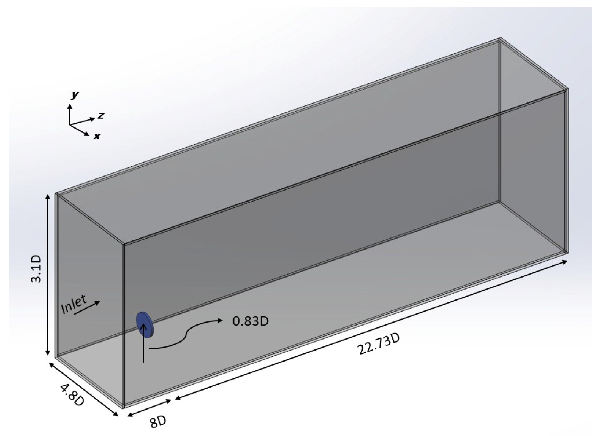
2.4. Computational Settings

Ansys-FLUENT 2020 R2 was chosen as the solver for this study. The domain of the study is a $31D\times 4.8D\times 3.1D$ box with the turbine located at 8D from the inlet. Given the choice of SST k-$\omega$ as the turbulence model, an inflation layer was used at the bottom surface. The results showed the value of $y^{+}<1$ in all of the adjacent wall cells. A general view of the domain is shown in Figure 1:

The domain dimensions have been chosen according to similar studies in the Saint Anthony Falls Laboratory [33]. A larger domain of $31D\times 8D\times 6.8D$ was also used to study the profiles in the wake and minimal differences between the results of the two domains were observed. The grid was refined upstream and especially downstream of the disk, and a super-refined grid was implemented inside the disk. The grid is made up of about one million cells. The boundary condition for this simulation consists of an inlet velocity profile at the inlet, a pressure outlet with zero gradients, no-slip condition at the bottom boundary, fixed velocity and turbulence intensity at the upper boundary, and symmetry condition at the lateral walls.

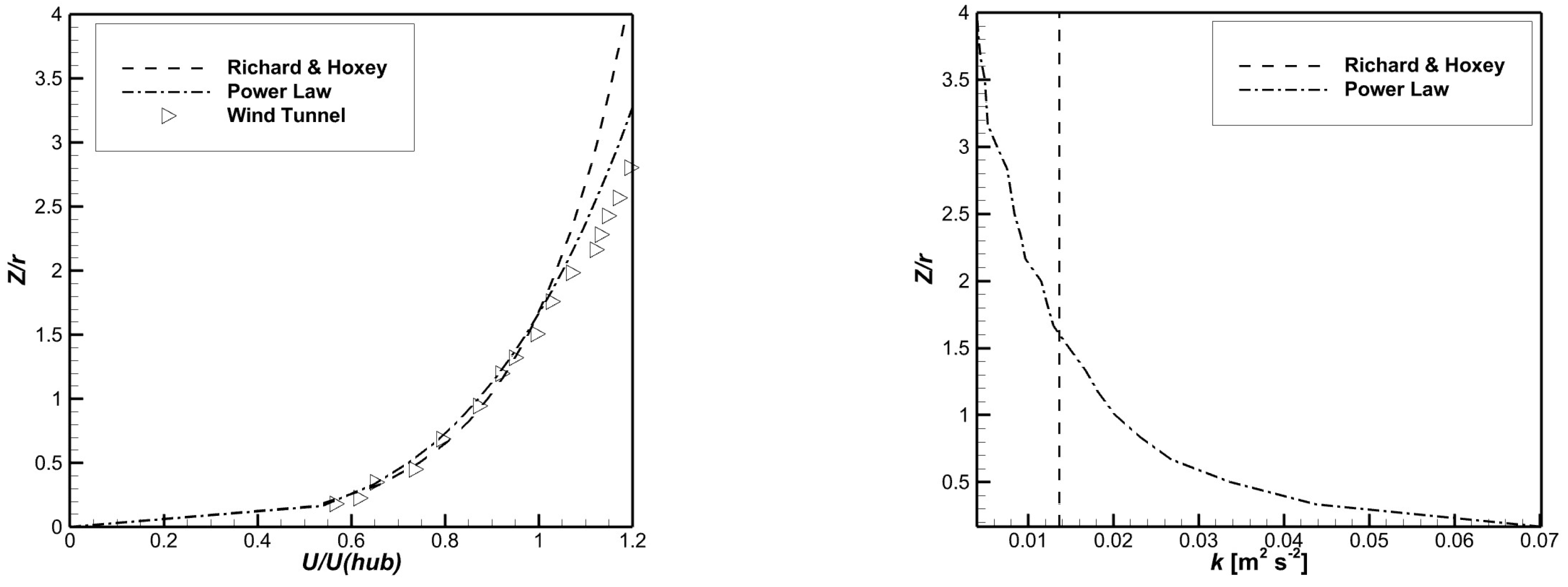
2.4.1. Inflow Conditions

Two sets of profiles were studied at the intake, as previously indicated. By making use of the Richard & Hoxey equation, (4)–(7) [11] and employing the experimental friction velocity and surface roughness, the logarithmic profile can be calculated:

$$U\left(y\right)=\frac{u_{*}}{\kappa }ln\left(\frac{y+y_0}{y_0}\right)$$

(4)

$$k\left(y\right)=\frac{u_{*}^3}{\sqrt{c_{\mu }}}$$

(5)

$$ϵ\left(y\right)=\frac{u_{*}^3}{\kappa (y+y_0)}$$

(6)

$$\omega =\frac{ϵ}{k{c}_{\mu }}$$

(7)

where $c_{\mu }$ is the model constant, $\kappa$ is the von-Kármán constant, $u_{*}$ is the friction velocity and $y_0$ is the surface roughness length.

An alternative method is to obtain a formula for velocity and turbulent kinetic energy using the power law equations:

$$U\left(z\right)=U_{ref}{\left(\frac{z}{z_{hub}}\right)}^{\alpha }$$

(8)

$$T_I\left(z\right)=0.1{\left(\frac{z}{z_{hub}}\right)}^{-\alpha -0.05}$$

(9)

$$k\left(z\right)=\frac{3}{2}{\left[U\left(z\right)TI\left(z\right)\right]}^2$$

(10)

$$ϵ\left(z\right)=\alpha c_{\mu }^{1/2}\frac{U_{ref}}{z_{hub}}{\left(\frac{z}{z_{hub}}\right)}^{\alpha -1}$$

(11)

where $U_{ref}$ is the inlet velocity at the hub height, $T_I$ is the turbulent intensity, and the terrain roughness is used to calculate the power law coefficient, $\alpha$. A value of $\alpha =0.27$ was chosen to recreate the rough wall velocity profile using the roughness classification of Uchida [40]. Figure 2 depicts the velocity and kinetic energy profiles at the inlet. It should be mentioned that these equations are only valid in the case of isotropic turbulence, and different formulations should be implemented if one were to use the anisotropic models, such as the RSM, for closure.

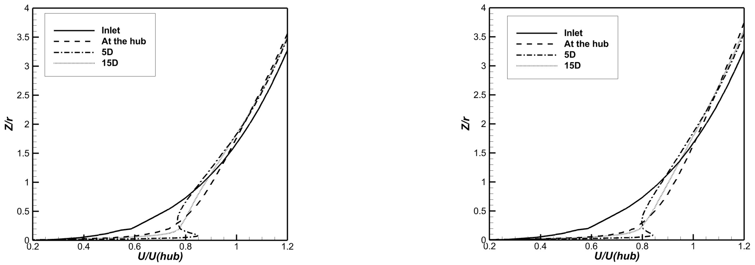
2.4.2. Horizontal Homogeneity

In order to have an accurate representation of the neutral atmospheric boundary layer, the horizontal homogeneity of the flow must be kept in check. Multiple methods of achieving homogeneity exist, including explicit modeling of the roughness element, minimization of upstream domain length, and more [41]. An additional wall shear stress condition was imposed on the wall (located between the inlet and the turbine) to tackle this problem. This method ensures that wall friction velocity is equal to ABL’s friction velocity, and as a result, the discrepancy is limited to 5% [41]. The wall shear is calculated using Equation (12):

$${\tau }_w=\rho {\left(u_{abl}^{*}\right)}^2$$

(12)

where $u_{abl}^{*}$ is the friction velocity of the boundary layer.

3. Results and Discussion

In this section, the results of the numerical simulation are presented. Firstly a set of simulations were conducted to study the development of the neutral atmospheric boundary layer in the absence of the wind turbine (Figure 3).

The over-prediction of the horizontal velocity in regions close to the wall is associated with the constant shear condition imposed between the disk and inlet instead of the no-slip condition. This is to ensure that the friction velocity of the simulation is equal to the wind tunnel experiment. In the upcoming sections, a study of the inflow profiles, followed by the study of the actuator disk thickness, will be presented.

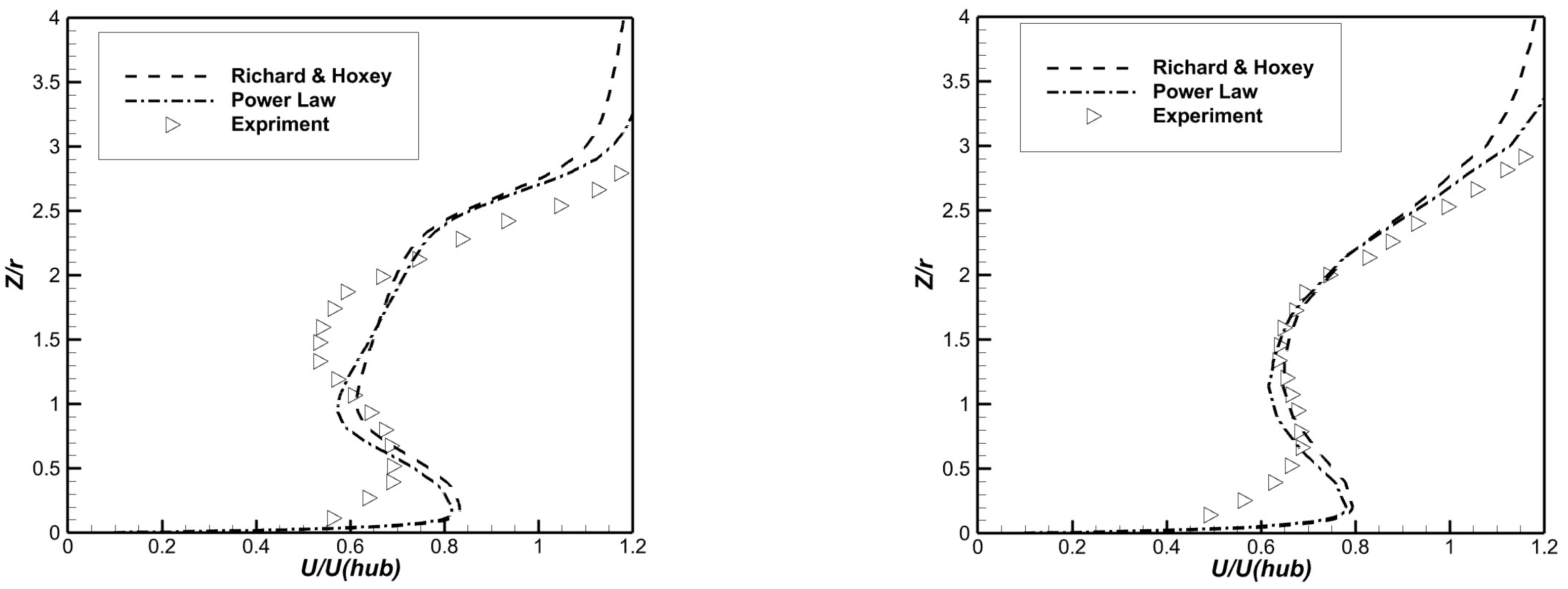
3.1. A Study of Inflow Parameters

As mentioned, the experimental data are collocated at four downstream cross-sections. From Figure 4, the rough wall velocity profiles in the near wake can be seen. The simple AD-no rotation model does not account for the pressure drop brought on by the swirl and the rotation of the flow, and as a result, the velocity profile is over-predicted in the near wake, as seen in this figure. The same type of behavior has also been observed in other sources [31]. Furthermore, the current model replaces not only the blades but the hub and the tower altogether. The interaction between the wind and tower also induces a velocity deficit in the wake, which causes an additional over-prediction of the velocity in the wake. The essence of the wake is closely simulated by both profiles. However, the power law appears more acceptable in both cross sections.

A phenomenon that is captured both by the numerical data and the experimental data is the symmetry of the velocity profile. This can be better seen in Figure 5 where the velocity deficit profiles show symmetry, with the deficit reaching its peak just above hub height. The $r^{*}$ parameter in Figure 5 is the non-dimensionalized vertical location with $r^{*}=0$ being the center of the actuator disk and r is the radius of the actuator disk. This is interesting, given that the incoming velocity profile is clearly asymmetrical. The same type of behavior is also evident in the experimental data. The symmetry seems to be less evident in the regions with $r^{*}=0>1.5$. Although both methods do over- and under-predict the velocity profile at different horizontal locations, overall, the profiles of the velocity deficit are fairly accurate with an error of <5% for $|r^{*}=0|>0.5$ and an error of 5% to 20% for $|r^{*}=0|<0.5$. The peak deficit is under-predicted by ∼20%, but the symmetrical behavior of the profile is evident in both cases. The reason for the under-predication of the peak velocity deficit is due to the absence of the wake rotation and tower. This under-prediction could be accounted for by using the LES/BEM [6] methods or by increasing the axial thrust of the disk by adding a drag force that accounts for the presence of the tower and hub. Similar to the velocity profiles, the accuracy of the results increases at $x/d=5$, where all three profiles overlap. By comparing the curves presented in Figure 5, it can also be deduced that the wake momentum deficit is gradually being refilled/smoothed in the far wake from the nearby unaffected flow.

The accuracy of the simulation increases at greater distances from the rotor in the far wake (Z/r > 4D). As seen in Figure 6, the power law shows a closer fit to the experimental data in the far wake. This is expected given that the main reason for the inaccuracy of the results in the near wake was due to the viscous interaction of the turbine and the air and the fact that the rotation of the blades was not taken into account. Once the flow evolves to the far wake, the shear stress between the wake and free stream and turbulent diffusion help the wake to recover the velocity deficit by transferring momentum from the free stream, and as a result, the effects of the near wake become less and less pronounced. However, for the entire wake, we observe under-prediction of the velocity in regions closer to the wall. The reason for this inconsistency lies in the shear stress that was added to the ground (wall) between the inlet and the turbine to account for the horizontal homogeneity of the flow. The added shear stress does not account for the no-slip condition but does assure that the friction velocity of the wall is equal to that of the experiment.

The velocity deficit profile in the far wake is shown in Figure 7. By comparing Figure 5 and Figure 7, an interesting observation can be noted that the velocity profile in the far wake is flatter than upstream. While the velocity deficit profile in the near wake showed a clear symmetry with a bell shape, the velocity deficit in the far wake is similar to a top hot profile. The reason for this difference is that as the velocity profile is fully recovered, the difference between the far wake velocity and the inlet velocity gets smaller, which in turn, results in a smaller and smoother velocity deficit.

The turbulence intensity profiles, depicted in Figure 8, are under-predicted by both the inflow profiles, particularly at the hub height. Interestingly though, the Richard & Hoxey formulation seems to better capture the turbulence intensity changes in both the near and far wake. The inaccuracy of the current model is due to multiple reasons, including the absence of rotation in the model and the absence of a hub structure. However, the main reason for this inaccuracy is probably the viscous interaction of the flow with the rotor and the anisotropic nature of turbulence in the near wake. This would mean that isotropic turbulence models, including the two-equation eddy viscosity models, fail to accurately predict the turbulence intensity levels. This discrepancy has been pointed out by other researchers, and methods such as using a modified k-$\omega$ model have been proposed to improve the accuracy of the turbulence intensity in the near-wake [42]. Alternatively, anisotropic methods such as Reynolds stress models have proven to better simulate the turbulence intensity distribution and quantity [31].

Again it is seen that similar to the velocity deficit profiles, both turbulence intensity profiles yield better results in the far wake than in the near wake. In addition to wake recovery, the general decline in turbulence intensity and flow anisotropy is another factor contributing to the improvement in precision. Figure 6 and Figure 8 also show that the velocity and turbulence intensity profiles have mostly recovered their inlet values. The logarithmic profile thus exhibits a higher degree of agreement with the experimental data in Z > 5D, as shown. As a whole, the power law better matches the experimental velocity profiles, while the logarithmic profiles are more adapted to capture the turbulence characteristics, notably in the far wake.

Nevertheless, both models are successful in capturing the key characteristics of the wake. As seen from Figure 9, the presence of the actuator disk causes the energy to be extracted from the flow. This can be better understood by comparing the Figure 9a,b. Additionally, the deceleration of flow and the wake recovery is also depicted in Figure 9c, where flow fully recovers in the far wake.

3.2. Actuator Disk Thickness

Three different thickness ratios of $T/r=0.0032,0.0064,0.0016$ were selected to study the sensitivity of the results to the disc thickness. A thorough examination of the turbulence intensity and turbulent kinetic energy, depicted in Figure 10, shows significant consistency between the three cases. In the $1D$ and $2D$ sections, all three thickness ratios behave remarkably similarly, aside from a negligible difference in predicting the peak turbulent kinetic energy. The turbulence intensity contours corresponding to these ratios are depicted in Figure 11. This suggests that the value of the disc thickness has minimal bearing on the outcomes of actuator disc simulations. The reason for this is that the source term in the N-S equation, which accounts for the thrust, has a constant value. Meaning once the body force is multiplied by the volume of the disk, the result is the same in all three cases.

Nevertheless, two quantities are affected by the value chosen for the thickness ratio, the actuator disk’s mesh refinement, and the computational time of the simulation. As the disks get smaller, the disk volume also decreases, resulting in a larger volumetric body force. This suggests that the smaller disks experience a more substantial force discontinuity and would, therefore, a fine mesh is needed to model the sudden changes in the domain accurately. The previous studies have indicated that a mesh size of $\Delta x=0.1D$ would yield satisfactory results [43]. A $\Delta x=D/30$ was implemented in this study to ensure that the mesh is sufficiently refined inside the actuator disk. Figure 12 shows the mesh used for the three cases. The same structured mesh was used to study the rate of convergence in all cases. Ansys Fluent employs two methods of calculating the residuals, scaled and normalized. The global scaled method is a more suitable measure of convergence for the majority of the simulations [44]. The global scaled continuity residuals (GSCR) is calculated using the equation below:

$$\mathit{GSCR}=\frac{{\mathit{R}}_{\mathit{Iteration}\mathit{N}}^{\mathit{c}}}{{\mathit{R}}_{\mathit{Iteration}\mathit{5}}^{\mathit{c}}}$$

(13)

where $R_{IterationN}^c$ is the continuity residual at the current iteration and $R_{Iteration5}^c$ is the largest absolute value of the continuity residual in the first five iterations of the simulation, the scaled continuity residuals for the thinnest disc failed to reach the lower levels of convergence, with the code not able to reduce the continuity residuals below ${10}^{-6}$, while for the other cases it reached ${10}^{-7}$ in half the time, with the $T/r=0.0064$ case achieving satisfactory convergence in the shortest time. All of this suggests that, while the precise actuator disc thickness does not significantly influence the simulation outcome, choosing a thickness of $T/r>0.0032$ does aid in convergence and computing efficiency. Furthermore, relative thickness less than $0.0032$ should be avoided. It should be mentioned that these results were obtained using a mesh sizing of $\Delta x=D/30$ inside the disk, which is a third of the value recommended by researchers. A grid independence study was also conducted, and the results again showed that the cases $T/r<0.0032$ were the slowest to reach the proper limits of convergence.

4. Conclusions

Given the effects of the inflow condition on the accuracy of the CFD simulations, an investigation of the two popular formulations used in the neutral atmospheric boundary layer simulation has been conducted. By comparing the Richard & Hoxey logarithmic formulation and the Architectural Institute of Japan formulation with a set of wind tunnel experiments, it was found that the power law profile is the superior all-around inflow profile despite the fact that the logarithmic formulation is the most used. This accuracy of the power law formulation is better for the wake’s velocity profiles. In contrast, The logarithmic profile of Richard & Hoxey slightly outperformed the power law at simulating the turbulence intensity profile. Although the actuator disc model can accurately simulate the profiles of the far wake, it is imprecise in the near wake, and alternative methods should be implemented if the physics of the near wake is to be studied. Both inflow profiles successfully captured velocity profiles in regions with $x/d>5$, but the logarithmic profile underestimated the velocity recovery in the upper regions with $Z/r>2.5$. Finally, an analysis of the impact of actuator disc thickness on the simulation also showed that the outcome of the simulation is not significantly affected by the exact value of the actuator disk’s thickness. This study also suggests that implementing relatively small disks elongates the simulations’ run time, and a suitable choice of AD thickness helps increase the convergence rate and reduce computational resources.

References

1. IRENA. Future of Wind: Deployment, Investment, Technology, Grid Integration and Socio-Economic Aspects; Report; International Renewable Energy Agency: Abu Dhabi, United Arab Emirates, 2019. [Google Scholar]
2. Froude, R.E. On the Part Played in Propulsion by Difference in Pressure. Trans. Inst. Nav. Archit. 1889, 30, 390–423. [Google Scholar]
3. Sumner, J.; España, G.; Masson, C.; Aubrun, S. Evaluation of RANS/actuator disk modelling of wind turbine wake flow using wind tunnel measurements. Int. J. Eng. Syst. Model. Simul. 2013, 5, 147–158. [Google Scholar] [CrossRef]
4. Antonini, E.; Romero, D.; Amon, C. Improving CFD wind farm simulations incorporating wind direction uncertainty. Renew. Energy 2018, 133, 1011–1023. [Google Scholar] [CrossRef]
5. Glauert, H. Airplane Propellers. In Aerodynamic Theory: A General Review of Progress under a Grant of the Guggenheim Fund for the Promotion of Aeronautics; Durand, W.F., Ed.; Springer: Berlin/Heidelberg, Germany, 1935; pp. 169–360. [Google Scholar] [CrossRef]
6. Lin, M.; Porté-Agel, F. Large-Eddy Simulation of Yawed Wind-Turbine Wakes: Comparisons with Wind Tunnel Measurements and Analytical Wake Models. Energies 2019, 12, 4574. [Google Scholar] [CrossRef] [Green Version]
7. Lavaroni, L.; Watson, S.; Cook, M.; Dubal, M. A comparison of actuator disc and BEM models in CFD simulations for the prediction of offshore wake losses. J. Phys. Conf. Ser. 2014, 524, 012148. [Google Scholar] [CrossRef]
8. Sorrensen, J.N.; Shen, W.Z. Numerical Modeling of Wind Turbine Wakes. J. Fluids Eng. 2002, 124, 393–399. [Google Scholar] [CrossRef]
9. Troldborg, N. Actuator Line Modeling of Wind Turbine Wakes. Ph.D. Thesis, Technical University of Denmark, Lyngby, Denmark, 2009. [Google Scholar]
10. Richards, P.J.; Norris, S.E. Appropriate boundary conditions for computational wind engineering models revisited. J. Wind Eng. Ind. Aerodyn. 2011, 99, 257–266. [Google Scholar] [CrossRef]
11. Richards, P.J.; Hoxey, R.P. Appropriate boundary conditions for computational wind engineering models using the k-ϵ turbulence model. J. Wind Eng. Ind. Aerodyn. 1993, 46–47, 145–153. [Google Scholar] [CrossRef]
12. Japan, A.I.O. Guidebook for CFD Predictions of Urban Wind Environment; Architectural Institute of Japan: Tokyo, Japan, 2007. [Google Scholar]
13. Mattar, S.J.; Kavian Nezhad, M.R.; Versteege, M.; Lange, C.F.; Fleck, B.A. Validation Process for Rooftop Wind Regime CFD Model in Complex Urban Environment Using an Experimental Measurement Campaign. Energies 2021, 14, 2497. [Google Scholar] [CrossRef]
14. Kavian Nezhad, M.R.; Lange, C.F.; Fleck, B.A. Performance Evaluation of the RANS Models in Predicting the Pollutant Concentration Field within a Compact Urban Setting: Effects of the Source Location and Turbulent Schmidt Number. Atmosphere 2022, 13, 1013. [Google Scholar] [CrossRef]
15. Santo, G.; Peeters, M.; Van Paepegem, W.; Degroote, J. Effect of rotor–tower interaction, tilt angle, and yaw misalignment on the aeroelasticity of a large horizontal axis wind turbine with composite blades. Wind Energy 2020, 23, 1578–1595. [Google Scholar] [CrossRef]
16. Syed Ahmed Kabir, I.F.; Ng, E. Effect of different atmospheric boundary layers on the wake characteristics of NREL Phase VI Wind Turbine. Renew. Energy 2018, 130, 1185–1197. [Google Scholar] [CrossRef]
17. Cabezón, D.; Migoya, E.; Crespo, A. Comparison of turbulence models for the computational fluid dynamics simulation of wind turbine wakes in the atmospheric boundary layer. Wind Energy 2011, 14, 909–921. [Google Scholar] [CrossRef] [Green Version]
18. Pichandi, C.; Pitchandi, P.; Kumar, S.; Sudharsan, N.M. Improving the performance of a combined horizontal and vertical axis wind turbine for a specific terrain using CFD. Mater. Today Proc. 2022, 62, 1089–1097. [Google Scholar] [CrossRef]
19. Tian, W.; Zheng, K.; Hu, H. Investigation of the wake propagation behind wind turbines over hilly terrain with different slope gradients. J. Wind Eng. Ind. Aerodyn. 2021, 215, 104683. [Google Scholar] [CrossRef]
20. Song, Y.L.; Tian, L.L.; Zhao, N. Numerical simulation and model prediction of complex wind-turbine wakes. J. Chin. Inst. Eng. 2021, 44, 627–636. [Google Scholar] [CrossRef]
21. Ichenial, M.M.; Elhajjaji, A. A study of the wind turbine wake dynamics in the neutral boundary layer using large eddy simulation. Procedia Manuf. 2019, 32, 775–785. [Google Scholar] [CrossRef]
22. Naderi, S.; Parvanehmasiha, S.; Torabi, F. Modeling of horizontal axis wind turbine wakes in Horns Rev offshore wind farm using an improved actuator disc model coupled with computational fluid dynamic. Energy Convers. Manag. 2018, 171, 953–968. [Google Scholar] [CrossRef]
23. Sedaghatizadeh, N.; Kelso, R.; Cazzolato, B.; Ghayesh, M.; Arjomandi, M. The effect of the boundary layer on the wake of a horizontal axis wind turbine. Energy 2019, 182, 1202–1221. [Google Scholar] [CrossRef]
24. Tian, L.; Song, Y.; Zhao, N.; Shen, W.; Zhu, C.; Wang, T. Effects of turbulence modelling in AD/RANS simulations of single wind and tidal turbine wakes and double wake interactions. Energy 2020, 208, 118440. [Google Scholar] [CrossRef]
25. Uchida, T.; Taniyama, Y.; Fukatani, Y.; Nakano, M.; Bai, Z.; Yoshida, T.; Inui, M. A New Wind Turbine CFD Modeling Method Based on a Porous Disk Approach for Practical Wind Farm Design. Energies 2020, 13, 3197. Available online: https://www.mdpi.com/1996-1073/13/12/3197 (accessed on 1 November 2022). [CrossRef]
26. Boni Cruz, L.E.; Carmo, B. Wind farm layout optimization based on CFD simulations. J. Braz. Soc. Mech. Sci. Eng. 2020, 42, 433. [Google Scholar] [CrossRef]
27. Chiang, Y.C.; Hsu, Y.C.; Chau, S.W. Power Prediction of Wind Farms via a Simplified Actuator Disk Model. J. Mar. Sci. Eng. 2020, 8, 610. [Google Scholar] [CrossRef]
28. Hamlaoui, M.N.; Smaili, A.; Dobrev, I.; Pereira, M.; Fellouah, H.; Khelladi, S. Numerical and experimental investigations of HAWT near wake predictions using Particle Image Velocimetry and Actuator Disk Method. Energy 2022, 238, 121660. [Google Scholar] [CrossRef]
29. Rezaeiha, A.; Micallef, D. Wake interactions of two tandem floating offshore wind turbines: CFD analysis using actuator disc model. Renew. Energy 2021, 179, 859–876. [Google Scholar] [CrossRef]
30. Richmond, M.; Antoniadis, A.; Wang, L.; Kolios, A.; Al-Sanad, S.; Parol, J. Evaluation of an offshore wind farm computational fluid dynamics model against operational site data. Ocean. Eng. 2019, 193, 106579. [Google Scholar] [CrossRef]
31. Tian, L.; Song, Y.; Zhao, N.; Shen, W.; Wang, T. AD/RANS Simulations of Wind Turbine Wake Flow Employing the RSM Turbulence Model: Impact of Isotropic and Anisotropic Inflow Conditions. Energies 2019, 12, 4026. [Google Scholar] [CrossRef] [Green Version]
32. Creech, A.; Früh, W.G.; Maguire, A.E. Simulations of an Offshore Wind Farm Using Large-Eddy Simulation and a Torque-Controlled Actuator Disc Model. Surv. Geophys. 2015, 36, 427–481. [Google Scholar] [CrossRef] [Green Version]
33. Wu, Y.T.; Porté-Agel, F. Modeling turbine wakes and power losses within a wind farm using LES: An application to the Horns Rev offshore wind farm. Renew. Energy 2015, 75, 945–955. [Google Scholar] [CrossRef]
34. Moens, M.; Duponcheel, M.; Winckelmans, G.; Chatelain, P. LES of wind farm response to transient scenarios using a high fidelity actuator disk model. J. Phys. Conf. Ser. 2016, 753, 032053. [Google Scholar] [CrossRef]
35. Behrouzifar, A.; Darbandi, M. An improved actuator disc model for the numerical prediction of the far-wake region of a horizontal axis wind turbine and its performance. Energy Convers. Manag. 2019, 185, 482–495. [Google Scholar] [CrossRef]
36. Simisiroglou, N.; Karatsioris, M.; Nilsson, K.; Breton, S.; Ivanell, S. The Actuator Disc Concept in Phoenics. Energy Procedia 2016, 94, 269–277. [Google Scholar] [CrossRef]
37. Chamorro, L.; Porté-Agel, F. A Wind-Tunnel Investigation of Wind-Turbine Wakes: Boundary-Layer Turbulence Effects. Bound.-Layer Meteorol. 2008, 132, 129–149. [Google Scholar] [CrossRef] [Green Version]
38. Stevens, R.; Martínez-Tossas, L.; Meneveau, C. Comparison of wind farm large eddy simulations using actuator disk and actuator line models with wind tunnel experiments Turbulence Effects. Renew. Energy 2018, 116, 470–478. [Google Scholar] [CrossRef]
39. Chamorro, L.; Porté-Agel, F. Effects of Thermal Stability and Incoming Boundary-Layer Flow Characteristics on Wind-Turbine Wakes: A Wind-Tunnel Study. Bound.-Layer Meteorol. 2010, 136, 515–533. [Google Scholar] [CrossRef] [Green Version]
40. Uchida, T. Design Wind Speed Evaluation Technique in Wind Turbine Installation Point by Using the Meteorological and CFD Models. J. Flow Control. Meas. Vis. 2018, 6, 168–184. [Google Scholar] [CrossRef] [Green Version]
41. Blocken, B.; Stathopoulos, T.; Carmeliet, J. CFD simulation of the atmospheric boundary layer: Wall function problems. Atmos. Environ. 2007, 41, 238–252. [Google Scholar] [CrossRef]
42. Bouras, I.; Ma, L.; Ingham, D.; Pourkashanian, M. An improved k-ω turbulence model for the simulations of the wind turbine wakes in a neutral atmospheric boundary layer flow. J. Wind Eng. Ind. Aerodyn. 2018, 179, 358–368. [Google Scholar] [CrossRef] [Green Version]
43. Gargallo-Peiró, A.; Avila, M.; Owen, H.; Prieto-Godino, L.; Folc, A. Mesh generation, sizing and convergence for onshore and offshore wind farm Atmospheric Boundary Layer flow simulation with actuator discs. J. Comput. Phys. 2018, 375, 209–227. [Google Scholar] [CrossRef]
44. Ansys, Inc. Ansys Fluent User’s Guide; Ansys, Inc.: Canonsburg, PA, USA, 2022; p. 5864. [Google Scholar]
Figure 1. Numerical domain.
Wind 02 00038 g001
Figure 2. Power law and logarithmic profiles at the inlet, velocity profile (left) and turbulence kinetic energy ( m 2 / s 2 ) (right).
Wind 02 00038 g002
Figure 3. Development of power law (left) and logarithmic velocity profile (right) in the absence of the actuator disk.
Wind 02 00038 g003
Figure 4. Power law and logarithmic velocity profile in the near wake at 3 D (left) 5 D (right).
Wind 02 00038 g004
Figure 5. Power law and logarithmic velocity deficit profile in the near wake at 3 D (left) 5 D (right).
Wind 02 00038 g005
Figure 6. Power law and logarithmic velocity profile in the far wake at 10 D (left) 15 D (right).
Wind 02 00038 g006
Figure 7. Power law and logarithmic velocity deficit profile in the far wake at 10 D (left) 15 D (right).
Wind 02 00038 g007
Figure 8. Turbulence Intensity at 3 D 5 D 10 D 15 D from left to right.
Wind 02 00038 g008
Figure 9. The velocity counter at (a) x y plane at z = 0.5 m (b) x y plane at z = 0.075 (c) at y z plane.
Wind 02 00038 g009
Figure 10. Turbulence kinetic energy ( m 2 / s 2 ) at 1 D (left) and 2 D (right).
Wind 02 00038 g010
Figure 11. Turbulence intensity at z = 1 D (a) T / r = 0.0016 (b) T / r = 0.0032 (c) T / r = 0.0064 .
Wind 02 00038 g011
Figure 12. The domain mesh (a) isometric view (b) side view of the domain at the disk (c) disk.
Wind 02 00038 g012