Entangled Dual Universe ^†

Abstract

Advances in cosmology and astronomical observations have brought to light significant tensions and uncertainties within the current model of cosmology, which assumes a spatially flat Universe and is known as the ΛCDM model. Moreover, the Planck Legacy 2018 release has preferred that the early Universe had a positive curvature with a confidence level more than 99%. This study reports a quantum mechanism that could potentially replace the concept of dark matter/energy by taking into the account the primordial curvature while generating the present-day spatial flatness. The approach incorporates the primordial curvature as the background curvature to extend the field equations into brane-world gravity. It utilizes a new wavefunction of the Universe that propagates in the bulk with respect to the scale factor and curvature radius of the early Universe upon the emission of the cosmic microwave background. The resulting wavefunction yields both positive and negative solutions, revealing the presence of a pair of entangled wavefunctions as a manifestation of the creation of matter and antimatter sides of the Universe. The wavefunction shows a nascent hyperbolic expansion away from early energy in opposite directions followed by a first decelerating expansion phase during the first ~10 Gyr and a subsequent accelerating expansion phase in reverse directions. During the second phase, both Universe sides are free-falling towards each other under gravitational acceleration. The simulation of the predicted background curvature evolution shows that the early curved background caused galaxies to experience external fields, resulting in the fast orbital speed of outer stars. Finally, the wavefunction predicts that the Universe will eventually undergo a rapid contraction phase resulting in a Big Crunch, which reveals a cyclic Universe.

1. Introduction

The Planck Legacy 2018 recent release implied a high confidence level of over 99% for a positively curved early Universe [1]. Efforts to recover spatial flatness by employing baryon acoustic oscillation data have encountered difficulties due to a discrepancy in the curvature parameter between the two datasets, which is 2.5 to 3σ [2].

Despite the success of the ΛCDM model of a spatially flat Universe, it masks large areas of ambiguity [3]. It is built upon vague components, namely, inflation, dark matter, and dark energy that have not been identified or fully understood despite extensive research efforts over decades. It leaves numerous enigmas, including the inferred baryon asymmetry, coincidence, cosmological constant problems, etc. Moreover, advances in cosmology and the enhanced precision of observations revealed inconsistencies among the essential parameters of the model—notably, the Hubble tension at 4 to 6σ [4].

The objective of this paper is to tackle the issues related to the Universe’s accelerated expansion and the high speed of the outer stars by adopting a quantum approach. Instead of the concept of dark matter/energy, this paper considers a quantum mechanism that is consistent with the preferred positively curved early Universe while yielding the present-day spatial flatness.

2. Interaction Field Equations

The Planck Legacy 2018 release preferred a closed early Universe, which indicates a curved early bulk. By considering the bulk effect, an extended action is obtained as

$$S=E_D{{\displaystyle \int }}_C^{ }\left[\frac{R}{\mathcal{R}}+\frac{L}{\mathcal{L}}\right]\sqrt{-g} d^4\rho$$

(1)

where $R$ and $\mathcal{R}$ are the localized and bulk curvatures, while $L$ and $\mathcal{L}$ are their Lagrangian densities, respectively. The bulk’s modulus, $E_D$, can be stated in terms of its resistance or field strength by using a Lagrangian formalism as $E_D=-{\mathcal{F}}_{\lambda \rho }{\mathcal{F}}^{\lambda \rho }/4{\mu }_0$. Due to bulk’s constant modulus and by considering its expansion, a dual action can be presented as

$$S={{\displaystyle \int }}_B^{ }\left[\frac{-{\mathcal{F}}_{\lambda \rho }{\tilde{g}}^{\lambda \gamma }{\mathcal{F}}_{\gamma \alpha }{\tilde{g}}^{\rho \alpha }}{4{\mu }_0}\right]\sqrt{-\tilde{g}} {{\displaystyle \int }}_C^{ }\left[\frac{R_{\mu \nu }{g}^{\mu \nu }}{{\mathcal{R}}_{\mu \nu }{\tilde{g}}^{\mu \nu }}+\frac{L_{\mu \nu }{g}^{\mu \nu }}{{\mathcal{L}}_{\mu \nu }{\tilde{g}}^{\mu \nu }}\right]\sqrt{-g} d^4\rho d^4\mathsf{\sigma }$$

(2)

Given that inducing a curvature requires high energy densities, it can be deemed that the bulk’s curvature (both induced and conformal) remains constant with respect to the quantum fields. Consequently, the action can be further expanded to

$$S={{\displaystyle \int }}_B^{ }\left[\frac{-{\mathcal{F}}_{\lambda \rho }{\tilde{g}}^{\lambda \gamma }{\mathcal{F}}_{\gamma \alpha }{\tilde{g}}^{\rho \alpha }}{4{\mu }_0}\right]\sqrt{-\tilde{g}}{{\displaystyle \int }}_C^{ }\left[\frac{R_{\mu \nu }{g}^{\mu \nu }}{{\mathcal{R}}_{\mu \nu }{\tilde{g}}^{\mu \nu }}\right]\sqrt{-g} {{\displaystyle \int }}_Q^{ }\left[\frac{p_{\mu }{p}_v{q}^{\mu \nu }}{{\pi }_{\mu }{\pi }_v{g}^{\mu \nu }}+\frac{L_{\alpha \beta }{q}^{\alpha \lambda }{L}_{\lambda \gamma }{q}^{\beta \gamma }}{2{\chi }_0{\mathcal{L}}_{\mu \nu }{g}^{\mu \nu }}\right]\sqrt{-q} {\vartheta }^2{d}^{12}\mathsf{\sigma }$$

(3)

where the two entangled Lagrangian densities are denoted by $L_{\alpha \beta }{L}^{\alpha \beta }/2{\chi }_0$, while their respective four-momentum is represented by $p_{\mu }{p}^v$. The four-momentum for vacuum energy density is represented by ${\pi }_{\mu }{\pi }^v$. The derivation of Equation (2) in Ref. [5] results in

$$\frac{R_{\mu \nu }}{\mathcal{R}}-\frac{1}{2}\frac{R}{\mathcal{R}}{g}_{\mu \nu }-\frac{R{\mathcal{R}}_{\mu \nu }}{{\mathcal{R}}^2}+\frac{R\left({\mathcal{K}}_{\mu \nu }-\frac{1}{2}\mathcal{K}{\widehat{p}}_{\mu \nu }\right)-\mathcal{R}\left(K_{\mu \nu }-\frac{1}{2}K{\widehat{q}}_{\mu \nu }\right)}{{\mathcal{R}}^2}=\frac{{\widehat{T}}_{\mu \nu }}{{\mathcal{T}}_{\mu \nu }}$$

(4)

These interaction field equations indicate that the induced over conformal curvatures equals the imposed over vacuum energy densities. By transforming the bulk’s intrinsic, $\mathcal{R}$, and extrinsic, $\mathcal{K}$, curvatures in Ref. [5], the interaction field equations reduce to

$$R_{\mu \nu }-\frac{1}{2}R{\widehat{g}}_{\mu \nu }-\left(K_{\mu \nu }-\frac{1}{2}K{\widehat{q}}_{\mu \nu }\right)=\frac{8\pi G_{\mathcal{R} }}{c^4}{\widehat{T}}_{\mu \nu }$$

(5)

where ${\widehat{g}}_{\mu \nu }=g_{\mu \nu }+2{\mathcal{R}}_{\mu \nu }/\mathcal{R}-2{\stackrel{=}{g}}_{\mu \nu }$, which can be expressed as ${\widehat{g}}_{\mu \nu }=g_{\mu \nu }+2{\tilde{g}}_{\mu \nu }-2{\stackrel{=}{g}}_{\mu \nu }$ because ${\mathcal{R}}_{\mu \nu }/\mathcal{R}={\mathcal{R}}_{\mu \nu }/{\mathcal{R}}_{\mu \nu }{\tilde{g}}^{\mu \nu }={\tilde{g}}_{\mu \nu }$, is the conformally transformed metric. The implicit term $R{\mathcal{R}}_{\mu \nu }/\mathcal{R}=R{\tilde{g}}_{\mu \nu }\equiv \Lambda g_{\mu \nu }$ resembles the cosmological ‘constant’ or parameter term as the bulk conformal curvature while $G_{\mathcal{R} }$relies on the background curvature.

Whereas the above equations describe the behavior of particles, the corresponding wave duality can be expressed by utilizing Equation (3) (obtained in Ref. [5]), which gives

$${\widehat{p}}_{\mu }\psi -\frac{1}{2}{\widehat{p}}^{\nu }{\xi }_{\mu \nu }\psi -\left(J^{\mu }{A}_{\mu }-\frac{1}{2}{J}^{\mu }{A}^{\nu }{\zeta }_{\mu \nu }\right)\psi =\frac{\hslash G_{\mathcal{R}}}{2c^2{g}_R}{\widehat{\mathcal{T}}}_{\mu }\psi$$

(6)

where ${\widehat{p}}_{\mu }$ and ${\widehat{\mathcal{T}}}_{\mu }$ are the momentum and gravitational operators, respectively; ${\xi }_{\mu \nu }=q_{\mu \nu }+2{\tilde{q}}_{\mu \nu }-2{\stackrel{=}{q}}_{\mu \nu }$ is the quantum cloud’s conformally transformed metric and $g_R$ is the gravitational field strength of its parent cloud-world. By applying the quantum operators,

$$i\hslash {\gamma }^{\mu }{\partial }_{\mu }\psi -\frac{1}{2}i\hslash {\gamma }^{\mu }{\partial }^{\nu }{\xi }_{\mu \nu }\psi -\left(J^{\mu }{A}_{\mu }-\frac{1}{2}{J}^{\mu }{A}^{\nu }{\zeta }_{\mu \nu }\right){\psi }^{ }=\frac{1}{2}\frac{\hslash }{x^{\mu }}R{\partial }_R\psi$$

(7)

These quantized interaction field equations reduce to quantum electrodynamics in a flat spacetime background [5]. The interaction field equations have the ability to eliminate the singularities and meet the requirements of a conformal invariance theory.

3. The Wavefunction of the Universe

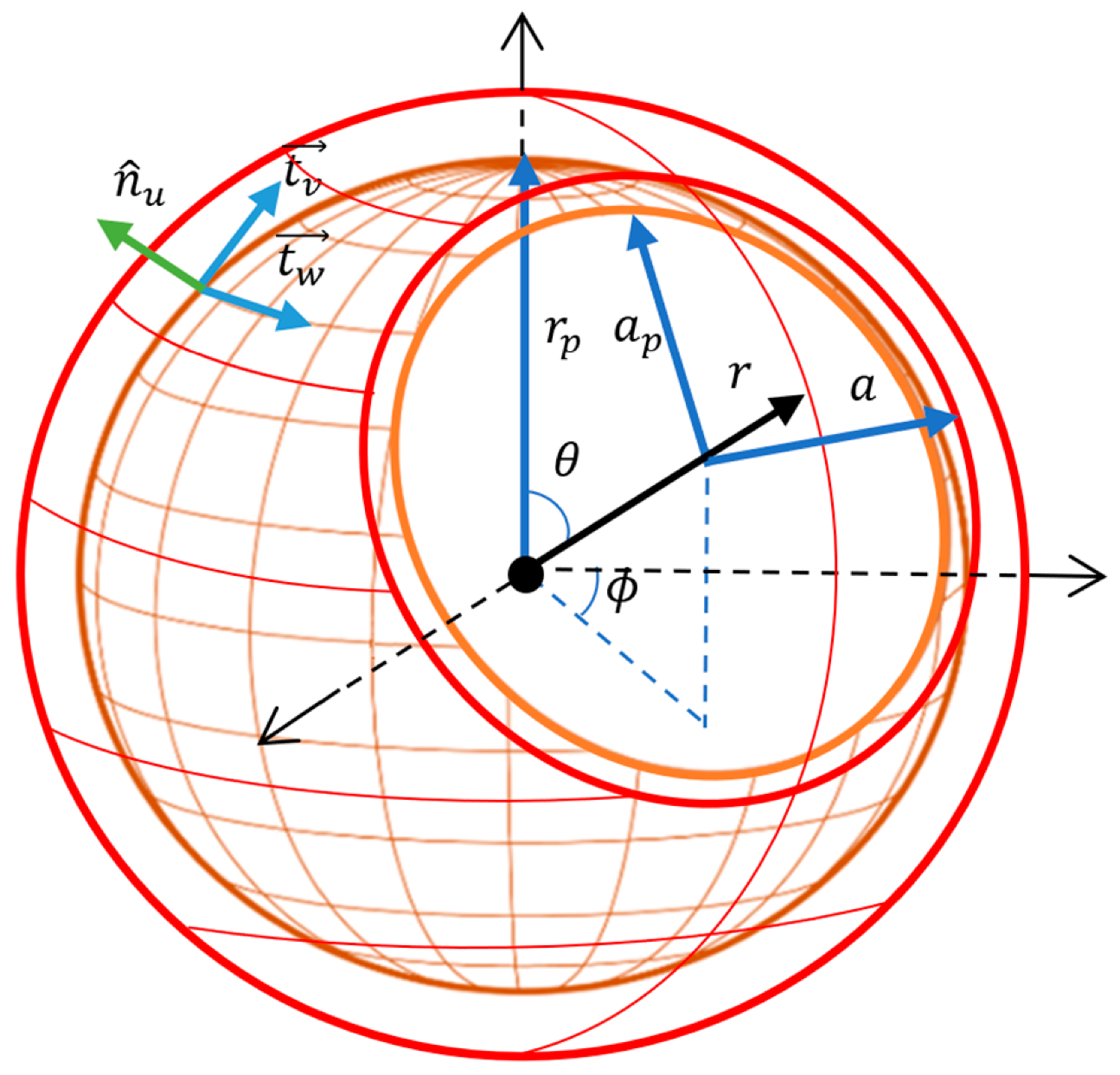
The standard Friedmann–Lemaître metric assumes an isotropic and homogenous Universe [6]. To reference it for a closed early Universe, a curvature radius $r_P$ when the CMB was emitted and the corresponding scale factor $a_P$ are integrated as in Figure 1.

The spacetime interval of this metric is

$$d{s}^2=c^{2 }d{t}^2-\frac{a^2\left(t\right)}{a_p{}^2}\left(\frac{d{r}^2}{1-r^2/r_p{}^2 }+r^{2 }d{\theta }^2+r^2{\sin }^2\theta d{\varphi }^2\right)$$

(8)

The hierarchical nature of the quantized field equations can be understood as signifying that a 4D conformal bulk, as a representation of vacuum energy of conformal time flow, embeds a 4D relativistic cloud-world representing a celestial object of conventional time flow that, in turn, encapsulates 4D relativistic quantum clouds of quantum time flow. As the quantum time is quantized in the conventional time, analogously, the latter should be quantized in the conformal time. The early Universe metric can be stated in terms of the conformal time as $d{s}^2=a^2/a_p{}^2\left(c^{2}d{\eta }^2-d{\tilde{r}}^2/(1-{\tilde{r}}^2/{\tilde{r}}_p{}^2)-{\tilde{r}}^{2}d{\theta }^2-{\tilde{r}}^2{\sin }^2\theta d{\varphi }^2\right)$.

To obtain the wavefunction of the Universe, referenced metric in terms of conformal time is substituted to the quantized field equations in Equation (7), as follows:

$$i\hslash {\gamma }^{\mu }{\partial }_{\mu }\psi -\frac{1}{2}i\hslash {\gamma }^{\mu }{\partial }^{\nu }\frac{a^2\left(\eta \right)}{a_p{}^2}\left(c^2-{\left(1-\frac{{\tilde{r}}^2}{{\tilde{r}}_p{}^2}\right)}^{-1}-{\tilde{r}}^2-{\tilde{r}}^2{\sin }^2\theta \right)\psi =\frac{\hslash G_{\mathcal{R}}}{2c^2{g}_R}{\widehat{\mathcal{T}}}_{\mu }\psi$$

(9)

Owing to the undeformed configuration of the early Universe, Equation (9) reduces to

$$i\hslash {\gamma }^{\mu }{\partial }_{\mu }\frac{a^2\left(\eta \right)}{a_p{}^2}\left(c^2-{\left(1-\frac{{\tilde{r}}^2}{{\tilde{r}}_p{}^2}\right)}^{-1}-{\tilde{r}}^2-{\tilde{r}}^2{\sin }^2\theta \right)\psi =\frac{\hslash R_p{}^2}{M_p{c}^2}{\mathcal{T}}_{\mu }\psi$$

(10)

where $g_p=M_p{G}_p/R_p{}^2$ is the gravitational field strength of the early Universe of mass $M_p$ and extrinsic curvature radius $R_p$. Performing the four-gradient covariant derivative gives

$$\frac{a^2}{a_p{}^2}\left({\gamma }^{\eta }\left(E+i2\hslash \frac{{\dot{a}}^{ }}{a}\right)-{\gamma }^x{p}_{x}c-{\gamma }^y{p}_{y}c-{\gamma }^z{p}_{z}c-M_p{c}^2\right)A\left(E,p\right)\mathit{exp}i\left(E,p\right)=0$$

(11)

where the metric coordinates are transformed into cartesian coordinates.

By applying the gamma matrices, ${\gamma }^{\mu }$, the wavefunction of the Universe is

$${\psi }_{\mu }\left(\eta \right)=\left(\begin{array}{cccc}\left(\begin{array}{c}\begin{array}{c}1\\ 0\end{array}\\ \begin{array}{c}\frac{p_{z}c}{E+M_p{c}^2+i2hH}\\ \frac{p_{x}c+i{p}_{y}c}{E+M_p{c}^2+i2hH}\end{array}\end{array}\right)& 0& 0& 0\\ 0& \left(\begin{array}{c}\begin{array}{c}0\\ 1\end{array}\\ \begin{array}{c}\frac{p_{x}c-i{p}_{y}c}{E+M_p{c}^2+i2hH}\\ \frac{-p_{z}c}{E+M_p{c}^2+i2hH}\end{array}\end{array}\right)& 0& 0\\ 0& 0& \left(\begin{array}{c}\begin{array}{c}\frac{p_{z}c}{E-M_p{c}^2+i2hH}\\ \frac{p_{x}c+i{p}_{y}c}{E-M_p{c}^2+i2hH}\end{array}\\ \begin{array}{c}1\\ 0\end{array}\end{array}\right)& 0\\ 0& 0& 0& \left(\begin{array}{c}\begin{array}{c}\frac{p_{x}c-i{p}_{y}c}{E-M_p{c}^2+i2hH}\\ \frac{-p_{z}c}{E-M_p{c}^2+i2hH}\end{array}\\ \begin{array}{c}0\\ 1\end{array}\end{array}\right)\end{array}\right) \mathit{exp}i\left(\frac{-R_p^{ 2}{\mathcal{T}}_{\mu }{x}^{\mu }}{M_p{c}^2}-2H\eta \right)$$

(12)

where $H={\dot{a}}^{ }/a$ is the Hubble parameter and $\eta =a_p\int dt/a$ is the conformal time.

To obtain the Hubble parameter and its evolution, Christoffel symbols are utilized for the referenced metric in Appendix A. The resultant Ricci tensor components are

$$\begin{gathered} R_{tt}=-3\frac{\ddot{a}}{a}, R_{rr}=\frac{1}{c^2}\left(\frac{a\ddot{a}}{a_p{}^2}+\frac{2{\dot{a}}^2}{a_p{}^2}+\frac{2c^2}{r_p{}^2}\right)/\left(1-\frac{r^2}{r_p{}^2}\right), \\ {R}_{\theta \theta }=\frac{r^2}{c^2}\left(\frac{a\ddot{a}}{a_p{}^2}+\frac{2{\dot{a}}^2}{a_p{}^2}+\frac{2c^2}{r_p{}^2}\right), R_{\varphi \varphi }=\frac{r^2{\sin }^2\theta }{c^2}\left(\frac{a\ddot{a}}{a_p{}^2}+\frac{2{\dot{a}}^2}{a_p{}^2}+\frac{2c^2}{r_p{}^2}\right), \end{gathered}$$

(13)

The perfect fluid equation, $T_{\mu \nu }=\left(\rho +P/c^2\right) u_{\mu }{u}_{\nu }+P{g}_{\mu \nu }$, is used to derive the referenced Friedmann equations, by substituting the referenced metric and Equation (13) in the interaction field equations, which gives

$$H^2\equiv \frac{{\dot{a}}^2}{a^2}=\frac{8\pi G_{\mathcal{R}}\rho }{3}-\frac{c^2{a}_p^{ 2}}{a^2{r}_p^{ 2}}$$

(14)

$$\dot{H}\equiv \frac{\ddot{a}}{a}=-\frac{4\pi G_{\mathcal{R}}}{3}\left(\rho +3\frac{P}{c^2}\right)$$

(15)

By expressing Equation (14) in the parametric form of the conformal time, $d\eta =a_{p}d\tau /ia$ (where $\dot{a}=ida/d\tau$); hence, $d\eta =a_{p}da/a\dot{a}$ as

$${{\displaystyle \int }}_0^{\eta }d\eta ={{\displaystyle \int }}_0^{2\pi }{a}_p{\left(\frac{8\pi G_p{\rho }_p{a}_p^{ 3}}{3}a-\frac{c^2{a}_p^{ 2}}{r_p{}^2}{a}^2\right)}^{-1/2} da$$

(16)

where $\rho ={\rho }_p{a}_p{}^3/a^3$. By integrating, the evolution over the conformal time of both the dimensionless scale factor and the imaginary time, $\tau$, (by utilizing $d\tau =ida/H{a}_p$) are

$$\frac{a\left(\eta \right)}{a_p}=\frac{G_p{M}_p}{c^2{r}_p}\left(1-\cos \frac{c}{r_p}\eta \right), \tau \left(\eta \right)=i\frac{E_p}{6H{E}_D }\left(\frac{c}{r_p}\eta -\sin \frac{c}{r_p}\eta \right)+{\tau }_p$$

(17)

where $M_p=\frac{4}{3}\pi {\rho }_p{r}_p^{ 3}$ and $E_p$ are early Universe’s mass and energy density, respectively; the amplitude of imaginary time is expressed in terms of vacuum energy density, $E_D$.

According to energy conservation, ${\Delta }_v{T}^{uv}=0$; thus, $\frac{\dot{a}}{a}{T}_u^u+3\frac{\dot{a}}{a}\rho -i\frac{\partial \rho }{\partial \tau }=0$ and $3\left(\rho +\frac{P}{c^2}\right)\frac{\dot{a}}{a}-i\frac{\partial \rho }{\partial \tau }=0$. The evolution of matter density can be obtained by integrating these outcomes, which gives $\rho \left(\eta \right)=D_p{\left(1-\cos c\eta /r_p\right)}^{-3}$, where $D_p$ is a constant. By substituting this finding of matter density evolution and the scale factor in Equation (17) into Equation (15), the Hubble parameter evolution can be determined by integration as

$$H\left(\eta \right)=H_r\left(\frac{1}{5}{\cot }^5\frac{c}{2r_p}\eta +\frac{2}{3}{\cot }^3\frac{c}{2r_p}\eta +\cot \frac{c}{2r_p}\eta \right)+H_p$$

(18)

where $H_r$ and $H_p$ are constants. In addition, a minimal form of the wavefunction of the Universe regarding its reference value, ${\psi }_p$, can be stated in terms of the spatial scale factor and imaginary time as

$$\frac{\psi \left(\eta \right)}{{\psi }_p}=\mp \frac{E_p}{6E_D }{\left({\left(1-\cos \frac{c}{r_p}\eta \right)}^2+\frac{c^2}{H_{\eta }^{ 2}{a}_p^{ 2}}{\left(\frac{c}{r_p}\eta -\sin \frac{c}{r_p}\eta \right)}^2\right)}^{1/2}exp i{\cot }^{-1}\left|H\right|{\frac{a_p-a_p\cos c\eta /r_p }{c^2\eta /r_p-c\sin c\eta /r_p}}^{ }$$

(19)

where $E_p/6E_D$ is a new density parameter that is identified as the ratio of the early Universe energy density, denoted by $E_p$, and vacuum energy density, $E_D$.

4. Universe Evolution

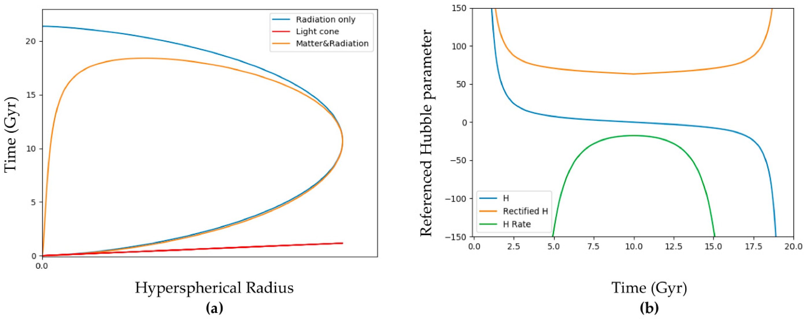
The wavefunction has two possible solutions, indicating the existence of two entangled wavefunctions representing separate matter and antimatter sides of the Universe. The integration constants of the model were set based on a mean evolution value of the Hubble parameter of $~70$km∙s⁻¹∙Mpc⁻¹ and a phase change occurring at 10 billion years.

The matter wavefunction, represented by the orange curve in Figure 2a, suggests that the evolution of the cosmos can be divided into three different phases. Both sides of the Universe expand away from the early energy state in the first phase. The expansion speed, represented by the blue curve in Figure 2b, initially increases at a hyperbolic rate but then starts to decrease during the first phase due to the gravitational attraction of the sides. It reaches its minimum at 10 billion years, marking the transition to the next phase.

In contrast, during the second phase, the matter wavefunction changes direction, and both sides move towards each other in a state of free-fall. Additionally, the expansion speed starts to increase in this phase, with the minus sign indicating the reverse direction.

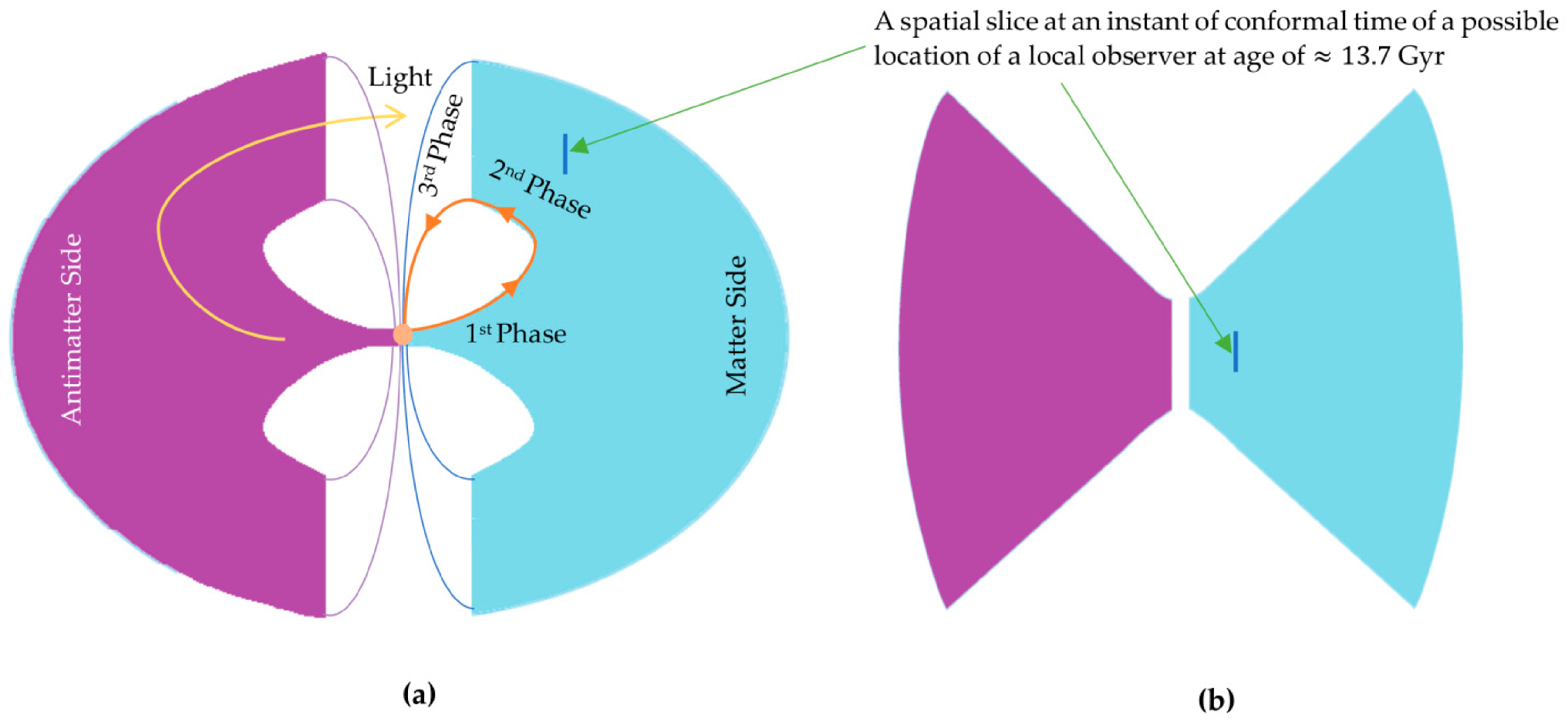
Interestingly, according to the matter wavefunction, there will be a final phase of spatial contraction occurring after approximately 18 billion years, which will lead to a Big Crunch, indicating a cyclic Universe. According to its wavefunction, radiation-only is predicted to propagate from one side to another, as shown in Figure 2a and Figure 3a; this phenomenon may explain why the CMB can be observed, despite propagating faster than matter.

Figure 3a illustrates a representation of the wavefunction, which can also explain the dark flow. Furthermore, Figure 3b convincingly duplicates the SLOAN Digital Sky Survey data visualization by displaying the apparent geometry of the Universe due to the effects of gravitational lensing.

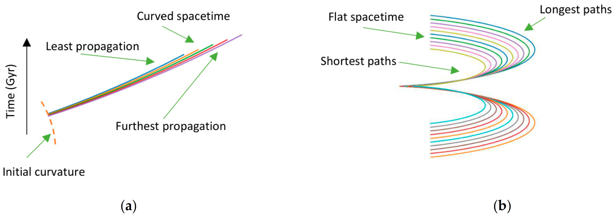
Figure 4a illustrates that when a set of spacetime paths were simulated with an initial positive curvature, the spacetime became curved during the first phase. This curvature indicates that the ends of the worldlines are not equal at any given moment in time. Conversely, during the second accelerated expansion phase in the reverse directions, the simulation of worldlines coupled with the initial positive curvature resulted in the ends of the worldlines being equal at all times, as shown in Figure 4b. This phenomenon occurs because the worldlines that covered the greatest distances in the first phase due to the positive curvature (Figure 4a) take the longest routes in the second phase, as shown in Figure 4b, due to their reverse directions, and the same is true for the reverse situation.

5. Galaxy Evolution and Rotation

The PL18 release suggests a background curvature that can be used in conjunction with the new interaction field equations to propose a new scenario for the formation of galaxies. This scenario involves a cloud-world that rotates and flows within a conformal bulk of an initial curvature. When calculating the entropy of a black hole using the semiclassical method, the boundary term is solely responsible for the entire influence [7]. By using this finding and reorganizing the field equations as

$$R_{\mu \nu }-\frac{1}{2}R{g}_{\mu \nu }-\frac{R{\mathcal{R}}_{\mu \nu }}{\mathcal{R}}=\frac{8\pi G_{\mathcal{R} }}{c^4}{\widehat{T}}_{\mu \nu }-\frac{R\left({\mathcal{K}}_{\mu \nu }-\frac{1}{2}\mathcal{K}{\widehat{p}}_{\mu \nu }\right)-\mathcal{R}\left(K_{\mu \nu }-\frac{1}{2}K{\widehat{q}}_{\mu \nu }\right)}{\mathcal{R}}=0$$

(20)

Equation (20) gives

$$R_{\mu \nu }=\frac{1}{2}R{g}_{\mu \nu }+R\frac{{\mathcal{R}}_{\mu \nu }}{\mathcal{R}}=\frac{1}{2}R\left(g_{\mu \nu }+2{\tilde{g}}_{\mu \nu }\right)=\frac{1}{2}R{g}_{\mu \nu }\left(1+2{\mathsf{\Omega }}^2\right)=\frac{1}{2}R{\widehat{g}}_{\mu \nu }=0$$

(21)

where ${\mathsf{\Omega }}^2$ is a conformal function as ${\tilde{g}}_{\mu \nu }=g_{\mu \nu }{\mathsf{\Omega }}^2$. The derived conformally transformed metric ${\widehat{g}}_{\mu \nu }=g_{\mu \nu }\left(1+2{\mathsf{\Omega }}^2\right)$ in Appendix B is

$$d{s}^2=\left(1-\frac{r_s }{r}-\frac{{\tilde{r}}_p}{\tilde{r}}\right)\left(-c^{2}d{t}^2+S^2\left(\frac{d{r}^2}{1+\frac{r_s{}^2 }{r^2}-2\frac{r_s }{r}}+\frac{r^{2}d{\theta }^2+r^2{\sin }^2\theta d{\varphi }^2}{1-\frac{r_s }{r}-\frac{{\tilde{r}}_p}{\tilde{r}}}\right)\right)$$

(22)

In a flat background ($\tilde{r}\to \infty )$, this metric reduces to the Schwarzschild metric, where the conformal function is ${\mathsf{\Omega }}^2=-\frac{{\tilde{r}}_p}{2\tilde{r}}/\left(1-\frac{r_s }{r}\right)$; here ${\tilde{r}}_p=2G_p{M}_p/c^2$ is the gravitational radius of the early Universe. The minus sign of ${\mathsf{\Omega }}^2$ indicates a spatial contraction through evolving in the conformal time as in a vortex model.

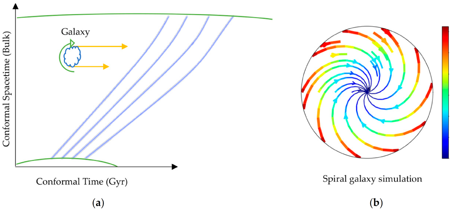
A study was carried out to examine how the background curvature affects the core of a galaxy. The simulation used a fluid to represent the spacetime continuum with curved paths that increased incrementally as the background curvature evolved as shown in Figure 5a. The findings from the simulation were then applied to create a model of a spiral galaxy, which is depicted in Figure 5b.

The simulation showed that the rotational velocity of a spiral galaxy’s outer regions is higher than that of its inner regions. This finding is consistent with observed rotational patterns of galaxies, except it used an ideal fluid.

6. Conclusions

This research shows that two entangled wavefunctions were created as an indication of the Universe’s separate matter and antimatter sides. Presently, as both sides fell freely towards each other under gravitational acceleration, this could be responsible for the effects linked to dark flow and dark energy. The predicted evolution of the background curvature shows that the outer stars move rapidly due to external fields exerted on them, which could account for the observed phenomena attributed to the dark matter. The wavefunction predicts that the Universe will eventually undergo a phase of rapid spatial contraction towards the end, culminating in a Big Crunch, implying that the Universe goes through cycles.

References

- Mokeddem, R.; Hipólito-Ricaldi, W.S.; Bernui, A. Excess of lensing amplitude in the Planck CMB power spectrum. arXiv 2022. [Google Scholar] [CrossRef]
- Handley, W. Curvature tension: Evidence for a closed universe. Phys. Rev. D 2021, 103, L041301. [Google Scholar] [CrossRef]
- Di Valentino, E.; Mena, O.; Pan, S.; Visinelli, L.; Yang, W.; Melchiorri, A.; Mota, D.F.; Riess, A.G.; Silk, J. In the realm of the Hubble tension—a review of solutions. Class. Quantum Gravity 2021, 38, 153001. [Google Scholar] [CrossRef]
- Dainotti, M.G.; De Simone, B.; Schiavone, T.; Montani, G.; Rinaldi, E.; Lambiase, G. On the Hubble Constant Tension in the SNe Ia Pantheon Sample. Astrophys. J. 2021, 912, 150. [Google Scholar] [CrossRef]
- Al-Fadhli, M.B. Celestial and Quantum Propagation, Spinning, and Interaction as 4D Relativistic Cloud-Worlds Embedded in a 4D Conformal Bulk: From String to Cloud Theory. Preprints 2023. [Google Scholar] [CrossRef]
- Ellis, G.F.R.; van Elst, H. Cosmological models (Cargese lectures 1998). In Theoretical and Observational Cosmology; Lachièze-Rey, M., Ed.; Kluwer: Dordrecht, The Netherlands, 1999; pp. 1–116. [Google Scholar]
- Dyer, E.; Hinterbichler, K. Boundary terms, variational principles, and higher derivative modified gravity. Phys. Rev. D 2009, 79, 024028. [Google Scholar] [CrossRef]
Figure 1.
The closed early Universe hypersphere. rp is the reference radius when the CMB was emitted and ap is the corresponding reference scale factor.
Figure 2.
(a) The diagram shows the matter wavefunction of one side of the Universe along with a radiation wavefunction and a light cone depicted by a straight line (not to scale). (b) The plot shows the Hubble parameter H.
Figure 3.
(a) A diagram representing the predicted topology of both sides. (b) The apparent topology in the first and second phases.
Figure 4.
The evolution of spacetime worldlines during two different time periods: (a) the early Universe and (b) the modern Universe.
Figure 5.
(a) The influence of the background curvature on the galaxy core. (b) A simulation of the rotation of a galaxy in a curved background, with the fastest tangential speeds shown in red.
Disclaimer/Publisher’s Note: The statements, opinions and data contained in all publications are solely those of the individual author(s) and contributor(s) and not of MDPI and/or the editor(s). MDPI and/or the editor(s) disclaim responsibility for any injury to people or property resulting from any ideas, methods, instructions or products referred to in the content. |
© 2023 by the author. Licensee MDPI, Basel, Switzerland. This article is an open access article distributed under the terms and conditions of the Creative Commons Attribution (CC BY) license (https://creativecommons.org/licenses/by/4.0/).
Share and Cite
MDPI and ACS Style
Al-Fadhli, M.B. Entangled Dual Universe. Phys. Sci. Forum 2023, 7, 56. https://doi.org/10.3390/ECU2023-14102
AMA Style
Al-Fadhli MB. Entangled Dual Universe. Physical Sciences Forum. 2023; 7(1):56. https://doi.org/10.3390/ECU2023-14102
Chicago/Turabian StyleAl-Fadhli, Mohammed B. 2023. "Entangled Dual Universe" Physical Sciences Forum 7, no. 1: 56. https://doi.org/10.3390/ECU2023-14102