
Quantum Gravitational Non-Singular Tunneling Wavefunction Proposal †


Department of Physics and Astronomy, Louisiana State University, Baton Rouge, LA 70803, USA
*
Author to whom correspondence should be addressed.
†
Presented at the 2nd Electronic Conference on Universe, 16 February–2 March 2023; Available online: https://ecu2023.sciforum.net/ .
Phys. Sci. Forum 2023, 7(1), 44; https://doi.org/10.3390/ECU2023-14101
Published: 2 March 2023
(This article belongs to the Proceedings of The 2nd Electronic Conference on Universe)
Abstract
:It has recently been shown that the tunneling wavefunction proposal is consistent with loop quantum geometry corrections, including both holonomy and inverse scale factor corrections, in the gravitational part of a spatially closed isotropic model with a positive cosmological constant. However, in the presence of inflationary potential, the initial singularity is kinetic-dominated, and the effective minisuperspace potential again diverges at the zero scale factor. As the wavefunction in loop quantum cosmology cannot increase towards the zero scale factor, the tunneling wavefunction seems incompatible. We show that consistently including inverse scale factor modifications, in scalar field Hamiltonian, changes the effective potential into a barrier potential, allowing the tunneling proposal. We also discuss the potential quantum instability of the cyclic universe, resulting from tunneling.
1. Introduction
Did the universe have a beginning? The answer to this question is affirmative in classical theory, due to singularity theorems proved by Penrose, Hawking and Geroch, in which they demonstrated that considering reasonable energy conditions, the universe must have begun from a Big Bang singularity in the past [1,2,3] (see also ref. [4] for a recent version of singularity theorem in inflationary cosmology). In classical general relativity (GR), singularities are the boundary of spacetime, where all physical laws break down, indicating the need for new physics. As the entire cosmos should be treated as a closed quantum system, the boundary conditions must be supplied as part of the dynamical laws. Several proposals have been put forward to describe the boundary conditions of the wavefunction of the universe leading to a self-contained universe, among which the tunneling wavefunction proposal [5,6] and the no-boundary wavefunction proposal [7,8] are the most successful. Although these proposals were formulated differently, they both can be described using Wheeler–DeWitt quantum cosmology as it was first studied in ref. [9]. Considering a closed isotropic universe with a cosmological constant , one can write the Wheeler–DeWitt equation as follows:
where a is the scale factor, the parameter n represents a factor ordering ambiguity, and is the effective minisuperspace potential.
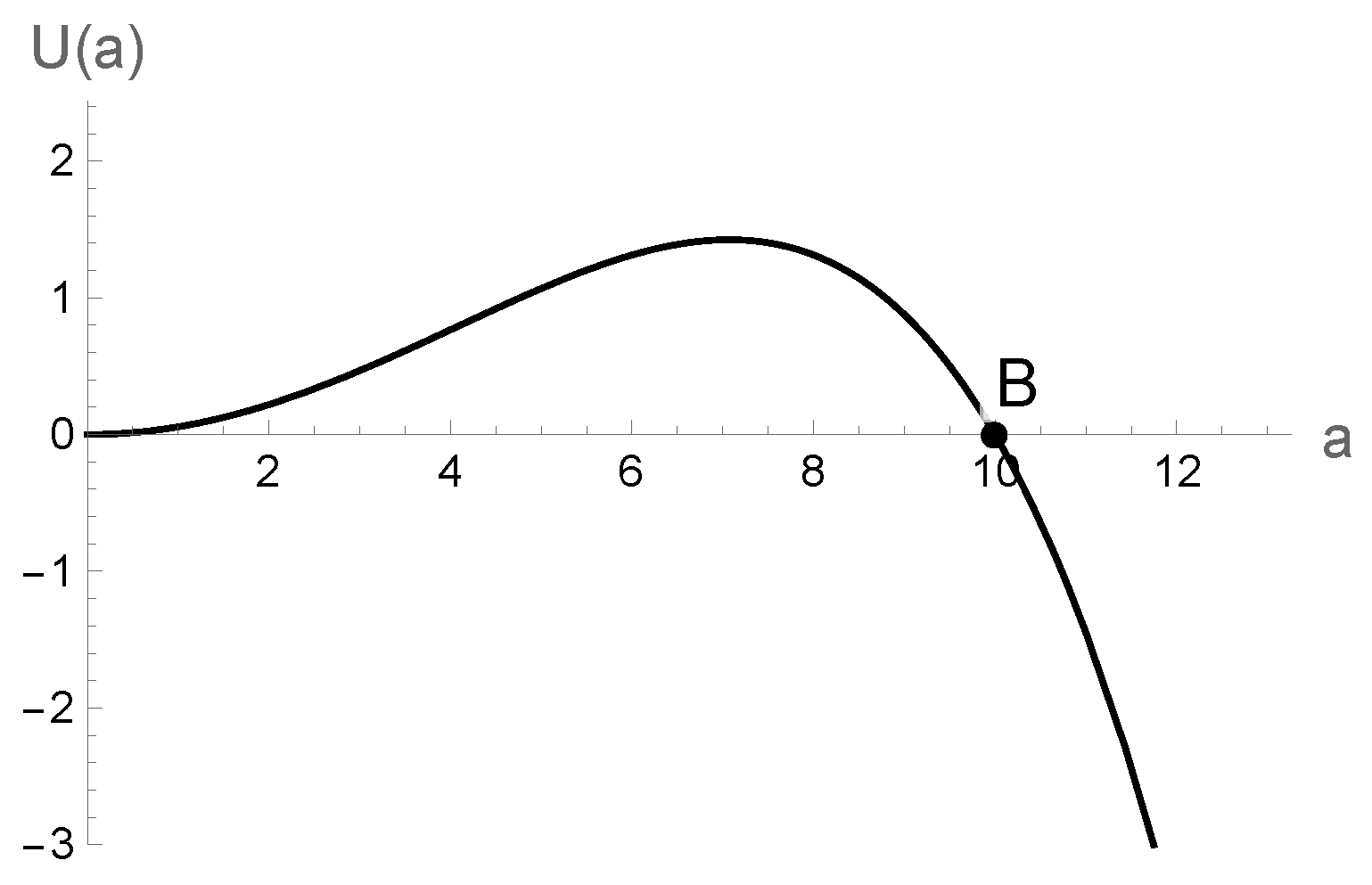
where and . Looking at Equation (1), one can see the similarity of the Wheeler–DeWitt equation to the Schrodinger equation with zero-energy eigenvalue. Moreover, from Figure 1, one can see that the effective minisuperspace potential has two regimes: the classically forbidden regime (the so-called Euclidian regime) and the classically allowed regime. In fact, the barrier shape of the effective minisuperspace potential manifests the analogy of the creation of the universe out of nothing via quantum tunneling phenomena. Classically, the universe contracts from a large size, bounces and expands. Quantum mechanically, the universe can start at the zero scale factor, with zero energy, i.e., nothing (“nothing” here means no space, time or matter), and then tunnel through the barrier to the classical expanding universe. As the potential has a barrier shape, the wavefunction is a superposition of growing and decreasing wave modes inside the barrier, while it is a superposition of oscillatory wave modes outside the barrier. By analogy with quantum tunneling, tunneling wavefunction describes the boundary conditions while the wavefunction has increasing wave mode towards the Big Bang and has only outgoing wave mode outside the barrier, like a particle escaping the radioactive nucleus. Using the WKB approximation, the wavefunction is given by [9]
where is the scale factor at which the universe bounces classically. However, the no-boundary proposal describes the boundary conditions of universe in such a way that the wavefunction has decreasing mode towards the Big Bang, inside the barrier, and it is in a superposition of ingoing (contracting universe) and outgoing (expanding universe) wave modes outside the barrier. Similarly, the wavefunction is given by [9]
where the wavefunction is real, which is a property of the no-boundary wavefunction. Given the wavefunction, the nucleation probability of the universe tunneling from nothing into a classical expanding universe reads as
where c is a positive constant, and the positive (negative) sign stands for the no-boundary (tunneling) proposal. From Equation (3), one can see that the nucleation probability peaks at a smaller value of the cosmological constant in the case of the no-boundary proposal, meaning that the universe favors tunneling to a large expanding universe, while the opposite is true for the tunneling boundary proposal. On the other hand, this means that the no-boundary proposal entails the largest probability of inflation happening at the minimum of potential, while the tunneling wave function entails the largest probability of inflation occurring at the top of hill of potential, which is theoretically and observationally favored. However, it has been proposed that the no-boundary proposal also predicts a large amount of inflation after multiplying nucleation probability by volume weighting [10].
Although these boundary proposals were successful in describing the boundary conditions of the universe, they were based on semi-classical physics. However, one must consider quantum gravity effects when the universe reaches the Planck regime. In fact, it is a reasonable question to ask how effective minisuperspace potential and boundary proposals are modified by the presence of quantum gravity effects. This issue was investigated in ref. [11] for a tunneling wavefunction proposal for a spatially closed universe in Loop Quantum Cosmology (LQC) with a positive cosmological constant (see refs. [12,13] for discussion about the no-boundary proposal in LQC). This analysis assumes the validity of effective spacetime description in LQC at all scales, resulting in modified Friedmann dynamics where quantum geometry effects originate from holonomy modifications and inverse scale factor modifications. In non-compact spatially flat models, the latter do not contribute, but they can be included in spatially compact and spatially curved models. In fact, for spatially curved anisotropic models, inverse scale factor effects play an important role in obtaining bounds on anisotropic shear [14]. It was found that taking into account only holonomy correction, the effective minisuperspace potential is lifted up at the zero scale factor, and the tunneling proposal becomes incompatible. However, at small scales, one needs to consider inverse scale factor correction together with holonomy correction, due to which the effective minisuperspace potential again recovers its barrier shape and the universe can also pick up the tunneling boundary conditions. Moreover, it was found that the universe can tunnel from nothing into either a classical expanding universe or a quantum cyclic universe, depending on how large the cosmological constant is.
The above results are valid only for the case of a pure cosmological constant; for inflation, one obtains a kinetic dominated phase as the singularity is approached [15]. The energy density behaves like that of a massless scalar field, as , and in the absence of any quantum, geometric modifications to energy density, the effective minisuperspace potential will diverge at the zero scale factor, seemingly making the tunneling wavefunction proposal inconsistent with loop quantum geometry effects. On the other hand, in the case of a cyclic universe, the universe can also tunnel back from bounce to the zero scale factor, indicating the quantum instability of a cyclic universe of this type in LQC. To understand this issue, let us note this instability in the Wheeler–DeWitt case. The effective minisuperspace potential in Equation (2) is approximated by in a small-scale factor regime: this means that any cyclic universe constructed using the cosmological constant, and perfect fluid with , is not stable against tunneling to the zero scale factor in Wheeler–DeWitt quantum cosmology [16,17,18]. However, ref. [19] notes that the effective minisuperspace potential for such a cyclic universe may be modified at small scales by Casimir energy, with lifting up the effective minisuperspace potential at the zero scale factor, stabilizing the cyclic universe against non-perturbative decay towards vanishing size. Therefore, those cyclic universes that are built from matter with are stable against tunneling to nothing in Wheeler–DeWitt quantum cosmology. However, the effective Friedmann equation in LQC is modified by quadratic energy density at high-energy limits, so the effective minisuperspace potential is approximated by [11]; therefore, it seems that a cyclic universe with may be stable against quantum decay to vanishing size in LQC. However, ref. [20] notes that even if one considers a massless scalar field, i.e., , there is a finite probability of tunneling back to the zero scale factor for an emergent/cyclic universe built in the context of LQC.
These results at first seem to contradict what was inferred from the effective minisuperspace potential found in ref. [11], if one includes a massless scalar field or any perfect fluid with . However, we show that this inconsistency stems from ignoring the small-scale factor regime effect of inverse scale factor correction for matter content. Therefore, the purpose of this manuscript is twofold: firstly, considering the cosmological constant plus a massless scalar field, to mimic the dynamics of inflationary cosmology, so as to investigate the possibility of creation of the universe out of nothing into an inflationary universe via the tunneling wavefunction proposal, taking into account the inverse scale factor correction for the massless scalar field; secondly, to study the quantum stability of cyclic universes, constructed using the cosmological constant and perfect fluid, in the context of LQC. An important caveat in including inverse scale factor modifications is that in a regime where inverse scale factor effects can play any role, the quantum fluctuations can be large, and effective description may become suspect. Surprisingly, however, the effect of large quantum fluctuations is to lower the density at which the bounce occurs in LQC [21,22]. In fact, for such states, the modified Friedmann dynamics are still valid, with the only change being the lowering of the bounce density [23]. Though the above results were obtained for a spatially flat model, they are also relevant to the model under consideration, because at small-scale factors the spatial curvature does not dominate in comparison to the energy density. In the next section, we discuss the effective dynamics of spatially closed LQC. Then, we derive the effective minisuperspace potential, including both holonomy and inverse scale factor corrections in Section 3, and discuss how adding a massless scalar field may change the effective minisuperspace potential of a small-scale regime. Finally, we give a summary of the results, and our conclusion.
2. k = 1 Loop Quantum Cosmology: Effective Dynamics
The canonical quantization in LQG is based on using Ashtekar–Barbero variables, due to which, one can express the field strength of the connection in the Hamiltonian constraint, in terms of the holonomies of the connection, which are computed over a loop with a minimum area determined by the quantum geometry. Applying LQG techniques to a symmetry-reduced isotropic universe, one obtains a quantum Hamiltonian constraint, which turns out to be a difference equation that results in singularity resolution [24,25,26,27,28,29]. Interestingly, the quantum dynamics in LQC can be captured accurately using an effective Hamiltonian constraint [30], which captures underlying quantum dynamics very accurately [31]. With both holonomy and inverse scale factor corrections, the modified Friedmann equation is
with and being the energy density of the cosmological constant and the massless scalar field, respectively, while is critical energy density, and
with . Furthermore, and are the inverse scale factor corrections for gravitational and matter sector, respectively, given by
where and is the Barbero–Immirzi parameter. Note that the and terms have been redefined, and they are not the original and terms in ref. [27]. One can check that Equation (4) reduces to the standard Friedmann equation, including the cosmological constant and massless scalar field at a large volume limit, where , and . We see from the modified Friedmann equation that the turnarounds of scale factor can be obtained from and . As a massless scalar field is proportional to , there may exist several distinct turnaround points, depending on the value of the cosmological constant and , as we see in the next section. However, the nature of the turnaround—whether it is a bounce or a recollapse or in the Einstein static phase—can be determined using the Raychaudhuri equation. The Raychaudhuri equation, which includes both holonomy and inverse scale factor corrections, is given by
with
where with . One can easily check that Equation (11) reduces to the Raychaudhuri equation in classical cosmology in a large volume limit. However, in a small-scale factor regime, , and ; hence, all terms containing and terms in the RHS of Equation (11) will be zero at the zero scale factor. The only non-vanishing term is the term with the cosmological constant, but at the zero scale factor, we have . Hence, one can find for , meaning that the universe is in Einstein static phase, even if one considers the cosmological constant with a massless scalar field. We will see that this will have significant implications for the tunneling wavefunction proposal in LQC.
3. Effective Minisuperspace Potential
In one-dimensional minisuperspace quantum cosmology, one can derive the effective minisuperspace potential either from Hamiltonian constraint or the Friedmann equation by an overall scaling, by powers of scale factor [11]. However, this analogy is true for only one-dimensional minisuperspace quantum cosmology. Similarly, having the effective Friedmann Equation (4), one can derive the effective minisuperspace potential, including both holonomy and inverse scale factor corrections, for the cosmological constant with a massless scalar field, as follows:
while it reduces to the effective minisuperspace potential found in Wheeler–DeWitt quantum cosmology, Equation (2), in large volume limit, with . In ref. [11], it was shown that in cases of a positive cosmological constant, i.e., , holonomy correction lifts the effective minisuperspace potential at the zero scale factor, excluding the possibility that the universe can be created out of nothing, satisfying tunneling boundary conditions. Including the inverse scale factor correction, i.e., the term, it was found that the effective minisuperspace potential recovers its barrier shape; hence, the universe can tunnel from nothing into an expanding universe or a quantum cyclic universe, satisfying tunneling boundary conditions. However, as we discussed in the introduction, the energy density of the inflation field becomes kinetically dominated at bounce, whereby the effective minisuperspace potential will diverge at the zero scale factor, indicating that the tunneling wavefunction is inconsistent with LQC. Moreover, those cyclic universes that are constructed by cosmological constant and matter content with seem to be stable against quantum decay to nothing, which contradicts the results found in ref. [20]. To investigate these issues, we considered a universe filled with the cosmological constant and a massless scalar field, with and without the inverse scale factor correction for the massless scalar field.
3.1.
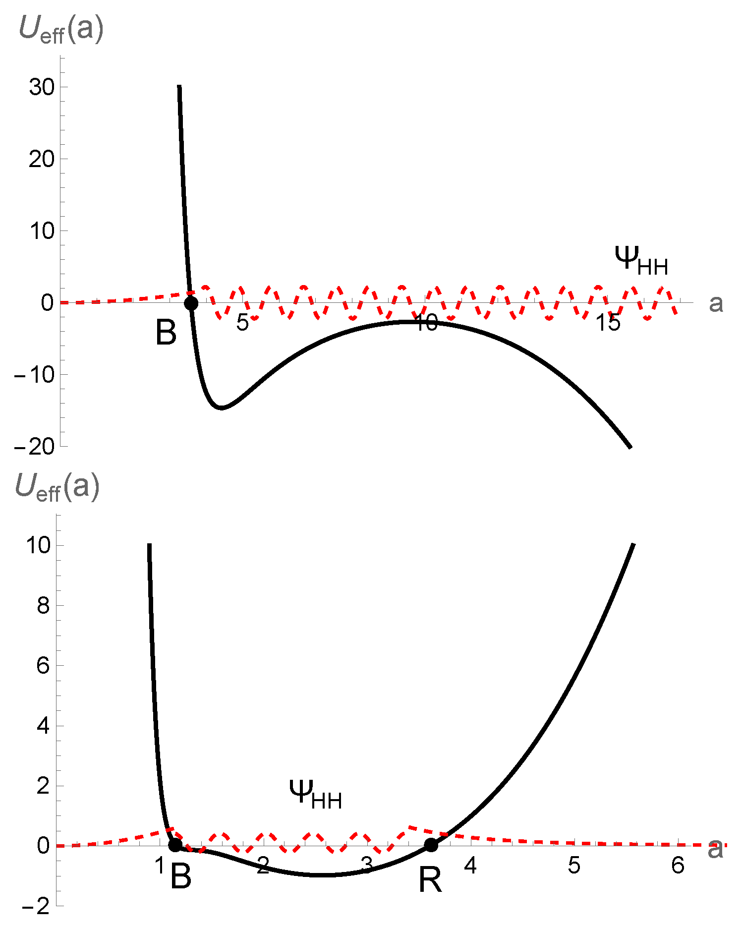
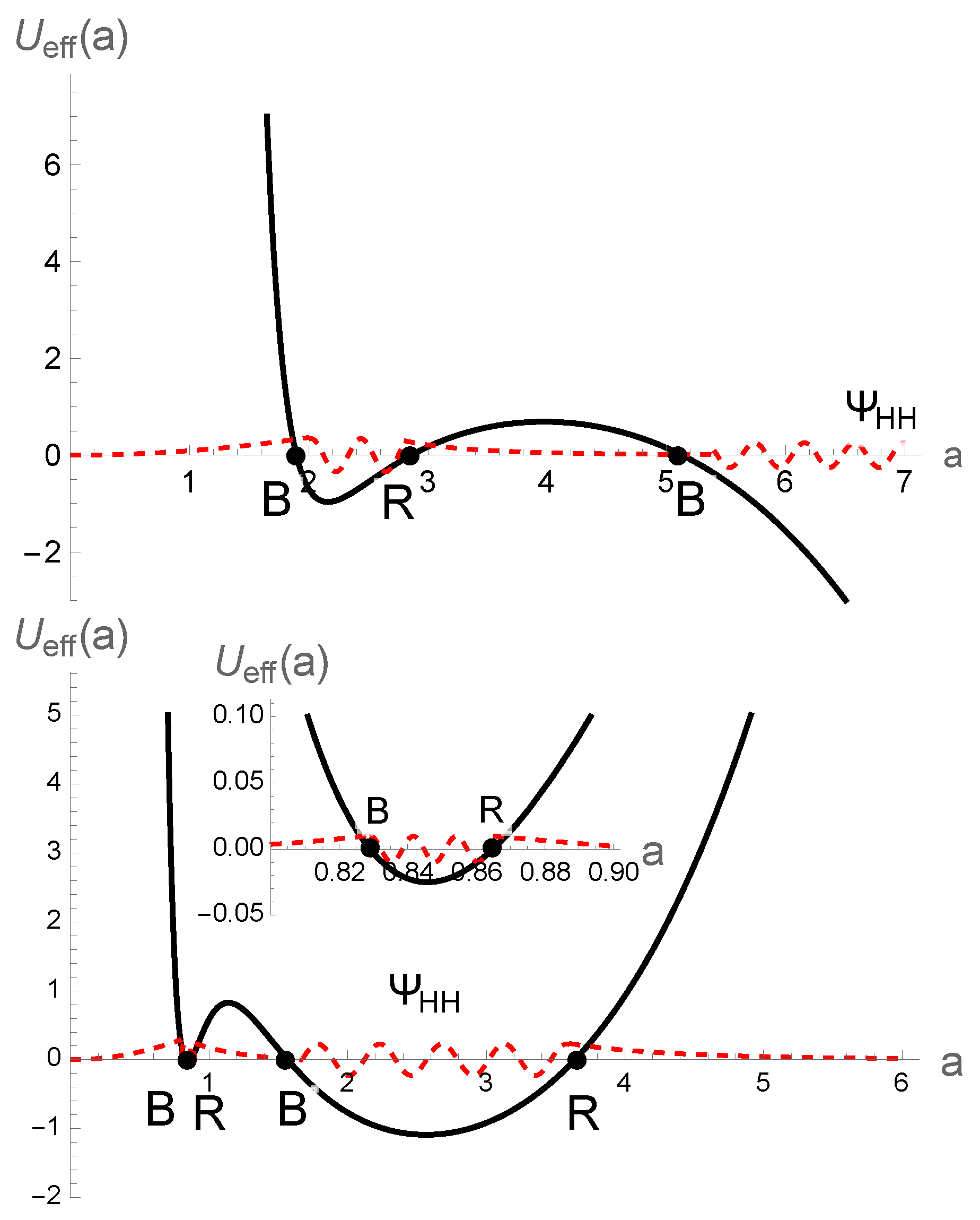
In this section, by ignoring the inverse scale factor correction for the energy density of the massless scalar field, i.e., , we plotted the effective minisuperspace potential for four different cases in Figure 2 and Figure 3. In fact, depending on the value of the cosmological constant and , the effective minisuperspace potential can have one, two, three or four turnaround points. However, the effective minisuperspace potential diverges at the zero scale factor in all four cases, meaning that the wavefunction should decrease towards the zero scale factor. Hence, the wavefunction cannot increase towards the zero scale factor, as a result of which the universe can be created from nothing, using the Hartle–Hawking boundary proposal (red dashed curve in Figure 2 and Figure 3) rather than the Vilenkin proposal. In the top panel of Figure 2, we plotted the effective minisuperspace potential for and , where it had just one bounce turnaround point: thereby, the universe is created out of nothing into a classical expanding universe, while in the bottom panel of Figure 2, we used the super-Planckian cosmological constant and , due to which the universe recollapses at a later point. However, this turnaround point has a quantum nature, so the universe can tunnel from nothing into a quantum cyclic universe in this case. In the top panel of Figure 3, we plotted the effective minisuperspace potential for and where it had three turnaround points. We found that the universe can tunnel from nothing into a cyclic universe, which can play the role of seed for creating a large expanding universe, as it tunnels from the barrier (similar to what was found in ref. [32]). Finally, in the bottom panel of Figure 3, we plotted the effective minisuperspace potential for and where it had four turnaround points. We found that the universe can tunnel from the zero scale factor into the first quantum cyclic universe, while from there it can also tunnel to the second quantum cyclic universe as it recollapses. We concluded that if one ignores the effect of inverse scale factor correction for matter content, the cyclic universe is stable against quantum decay to vanishing size, because the effective minisuperspace diverges at the zero scale factor, as we expected.
3.2.
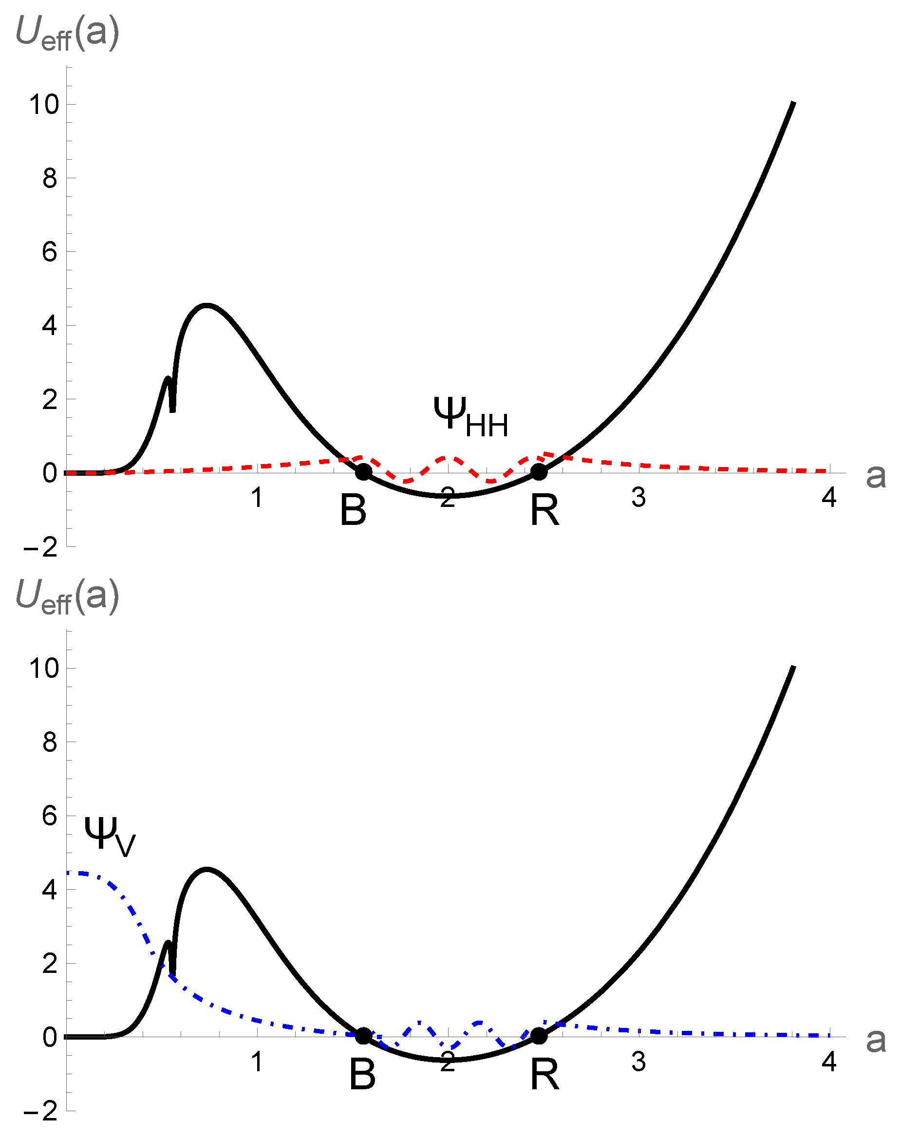
Although spacetime is non-singular in the presence of holonomy and inverse scale factor corrections, one needs to include inverse scale factor correction for a massless scalar field, especially in studying a tunneling wavefunction, because the universe is deep in the Planckian regime, i.e., . In this regime, , leading into non-trivial results. We plotted the effective minisuperspace potential in Figure 4 and Figure 5 for those values of the cosmological constant for which we had only one or two turnaround points. However, due to the complicated behavior of the term, several turnarounds points could be obtained like those we discussed in the previous section. Looking at Figure 4 and Figure 5, one can see that the effective minisuperspace potential (black curve) recovers its barrier shape, because for , as is the case in Wheeler–DeWitt quantum cosmology. Hence, the wavefunction can either pick up the decreasing or increasing wave mode inside the barrier. Therefore, the universe can tunnel from nothing into a classical expanding universe (Figure 4) or a quantum cyclic universe (Figure 5), satisfying either tunneling or no-boundary boundary conditions. One should point out that going into the zero scale factor does not contradict the prediction of LQC that spacetime is non-singular, although it does contradict the occurrence of bounce. On the other hand, as the universe is again able to tunnel back from bounce to the zero scale factor, the cyclic universe constructed from the cosmological constant and perfect fluid with is not stable against quantum decay to vanishing size, which is consistent with the results found in ref. [20].
To reach this conclusion, we used the effective Friedmann Equation (4), which is accurate when quantum fluctuations are small, while quantum fluctuation are large near to the Big Bang singularity for quantum tunneling; therefore, the effective dynamics are trustworthy near to the zero scale factor. However, the effects of such large quantum fluctuation on the accuracy of effective equations were thoroughly investigated in Refs. [21,22,23] for flat spacetime, in which they showed that such quantum fluctuation will change the upper bound of the maximum energy scale for which the bounce will occur in a flat isotropic universe. In fact, it was found that for generalized Gaussian states, the maximum energy density should be replaced by
where and , and it approaches when , assuming dispersion relation and . As the massless scalar field becomes dominated at the bounce, therefore, one can neglect the effect of the intrinsic curvature, so that it is legitimate to assume the same effect for close LQC in the presence of large quantum fluctuations for the case studied here. Therefore, large quantum fluctuations only lower the energy scale for which the bounce occurs. In other words, such large quantum fluctuations will change the height of the barrier, thereby changing the rate of nucleation probability.
4. Summary and Conclusions
In this manuscript, we investigated the possibility of creating the universe out of nothing via the tunneling wavefunction proposal, considering loop quantum geometry effects, while assuming the validity of effective dynamis in all regimes. As inflation energy density will be generally kinetically dominated at the bounce, we considered the cosmological constant, together with a massless scalar field, to mimic the inflationary cosmology. We found that, because the massless scalar field behaved as , it modified the effective minisuperspace potential at small-scale factor, producing an infinite wall; hence, the universe cannot tunnel from nothing into an expanding universe satisfying tunneling boundary conditions. However, in a small-scale factor regime, one should consider the effect of inverse scale factor correction for matter components which are proportional to the inverse of scale factor. We showed that by including the inverse scale factor correction for a massless scalar field, the effective minisuperspace potential recovered its barrier shape in a small-scale regime, and the tunneling wavefunction proposal could explain the initial conditions for the universe. Although effective dynamics are valid only for small quantum fluctuations, using generalized Guassian states, we noted that large quantum fluctuations only lead into a lower energy scale for the bounce to happen, as a result of which, the height of the barrier changes and the rate of nucleation probability also changes accordingly.
In addition, we also considered a cyclic universe, by choosing a large cosmological constant, due to which the universe recollapses at a late stage. It was shown in ref. [11] that the universe can tunnel from nothing into a cyclic universe for the pure de Sitter universe, including both holonomy and inverse scale factor corrections. However, as the universe recollapses, it can also tunnel back to the zero scale factor, indicating the quantum instability of a cyclic universe in the context of LQC. In fact, this is true for any cyclic universe which is constructed using the cosmological constant and matter component with . However, if one constructs cyclic universes with , such as a massless scalar field, the effective minisuperspace potential diverges at the zero scale factor, whereby the universe cannot tunnel from the zero scale factor to the cyclic universe, satisfying the tunneling boundary conditions. Accordingly, the universe cannot tunnel back from bounce to the zero scale factor, therefore, the cyclic universe is stable against quantum decay to vanishing size. However, in a small-scale factor regime, one must also consider inverse scale factor correction for matter components. We showed that, in this case, the universe is again able to tunnel from the zero scale factor into the cyclic universe, and tunnel back to the zero scale factor as it recollapses again, indicating the quantum instability of the cyclic universe in LQC. In fact, this is true for any cyclic universe that is constructed from the cosmological constant with perfect fluid, if we include inverse scale factor corrections for matter content.
Author Contributions
Conceptualization, M.M. and P.S.; software, Mathematica, validation, M.M. and P.S.; formal analysis, M.M. and P.S.; investigation, M.M. and P.S.; writing—original draft preparation, M.M. and P.S.; writing—review and editing, M.M. and P.S.; visualization, M.M. and P.S.; supervision, M.M. and P.S.; project administration, M.M. and P.S.; funding acquisition, P.S. All authors have read and agreed to the published version of the manuscript.
Funding
This work is supported by the NSF grant PHY-2110207.
Institutional Review Board Statement
Not applicable.
Informed Consent Statement
Not applicable.
Data Availability Statement
Not applicable.
Acknowledgments
This work is supported by the NSF grant PHY-2110207.
Conflicts of Interest
The authors declare no conflict of interest.
References
- Geroch, R.P. What is a singularity in general relativity? Ann. Phys. 1968, 48, 526–540. [Google Scholar] [CrossRef]
- Hawking, S.W.; Penrose, R. The Singularities of gravitational collapse and cosmology. Proc. Roy. Soc. Lond. A 1970, 314, 529–548. [Google Scholar]
- Hawking, S.W.; Ellis, G.F.R. The Large Scale Structure of Space-Time; Cambridge University Press: Cambridge, UK, 1973. [Google Scholar]
- Borde, A.; Guth, A.H.; Vilenkin, A. Inflationary space-times are incompletein past directions. Phys. Rev. Lett. 2003, 90, 151301. [Google Scholar] [CrossRef] [Green Version]
- Vilenkin, A. Creation of Universes from Nothing. Phys. Lett. B 1982, 117, 25–28. [Google Scholar] [CrossRef]
- Vilenkin, A. Quantum Creation of Universes. Phys. Rev. D 1984, 30, 509–511. [Google Scholar] [CrossRef]
- Hartle, J.B.; Hawking, S.W. Wave Function of the Universe. Phys. Rev. D 1983, 28, 2960–2975. [Google Scholar] [CrossRef]
- Hawking, S.W. The Quantum State of the Universe. Nucl. Phys. B 1984, 239, 257. [Google Scholar] [CrossRef]
- Vilenkin, A. Quantum Cosmology and the Initial State of the Universe. Phys. Rev. D 1988, 37, 888. [Google Scholar] [CrossRef]
- Hartle, J.B.; Hawking, S.W.; Hertog, T. No-Boundary Measure of the Universe. Phys. Rev. Lett. 2008, 100, 201301. [Google Scholar] [CrossRef] [PubMed] [Green Version]
- Motaharfar, M.; Singh, P. Tunneling wavefunction proposal with loop quantum geometry effects. arXiv 2022, arXiv:2212.14065. [Google Scholar]
- Brahma, S.; Yeom, D.H. No-boundary wave function for loop quantum cosmology. Phys. Rev. D 2018, 98, 83537. [Google Scholar] [CrossRef] [Green Version]
- Brahma, S.; Yeom, D.H. On the geometry of no-boundary instantons in loop quantum cosmology. Universe 2019, 5, 22. [Google Scholar] [CrossRef] [Green Version]
- Gupt, B.; Singh, P. Contrasting features of anisotropic loop quantum cosmologies: The Role of spatial curvature. Phys. Rev. D 2012, 85, 44011. [Google Scholar] [CrossRef] [Green Version]
- Foster, S. Scalar field cosmologies and the initial space-time singularity. Class. Quant. Grav. 1998, 15, 3485–3504. [Google Scholar] [CrossRef]
- Graham, P.W.; Horn, B.; Kachru, S.; Rajendran, S.; Torroba, G. A Simple Harmonic Universe. J. High Energy Phys. 2014, 2, 29. [Google Scholar] [CrossRef] [Green Version]
- Mithani, A.T.; Vilenkin, A. Collapse of simple harmonic universe. J. Cosmol. Astropart. Phys. 2012, 1, 28. [Google Scholar] [CrossRef]
- Mithani, A.; Vilenkin, A. Did the universe have a beginning? arXiv 2012, arXiv:1204.4658. [Google Scholar]
- Graham, P.W.; Horn, B.; Rajendran, S.; Torroba, G. Exploring eternal stability with the simple harmonic universe. J. High Energy Phys. 2014, 8, 163. [Google Scholar] [CrossRef] [Green Version]
- Mithani, A.T.; Vilenkin, A. Instability of an emergent universe. J. Cosmol. Astropart. Phys. 2014, 5, 6. [Google Scholar] [CrossRef] [Green Version]
- Corichi, A.; Montoya, E. Coherent semiclassical states for loop quantum cosmology. Phys. Rev. D 2011, 84, 44021. [Google Scholar] [CrossRef] [Green Version]
- Diener, P.; Gupt, B.; Megevand, M.; Singh, P. Numerical evolution of squeezed and non-Gaussian states in loop quantum cosmology. Class. Quant. Grav. 2014, 31, 165006. [Google Scholar] [CrossRef] [Green Version]
- Ashtekar, A.; Gupt, B. Generalized effective description of loop quantum cosmology. Phys. Rev. D 2015, 92, 84060. [Google Scholar] [CrossRef] [Green Version]
- Ashtekar, A.; Pawlowski, T.; Singh, P. Quantum Nature of the Big Bang: Improved dynamics. Phys. Rev. D 2006, 74, 84003. [Google Scholar] [CrossRef] [Green Version]
- Ashtekar, A.; Pawlowski, T.; Singh, P. Quantum nature of the big bang. Phys. Rev. Lett. 2006, 96, 141301. [Google Scholar] [CrossRef] [PubMed] [Green Version]
- Ashtekar, A.; Pawlowski, T.; Singh, P. Quantum Nature of the Big Bang: An Analytical and Numerical Investigation. I. Phys. Rev. D 2006, 73, 124038. [Google Scholar] [CrossRef] [Green Version]
- Ashtekar, A.; Pawlowski, T.; Singh, P.; Vandersloot, K. Loop quantum cosmology of k = 1 FRW models. Phys. Rev. D 2007, 75, 24035. [Google Scholar] [CrossRef] [Green Version]
- Ashtekar, A.; Corichi, A.; Singh, P. Robustness of key features of loop quantum cosmology. Phys. Rev. D 2008, 77, 24046. [Google Scholar] [CrossRef] [Green Version]
- Ashtekar, A.; Singh, P. Loop Quantum Cosmology: A Status Report. Class. Quant. Grav. 2011, 28, 213001. [Google Scholar] [CrossRef] [Green Version]
- Taveras, V. Corrections to the Friedmann Equations from LQG for a Universe with a Free Scalar Field. Phys. Rev. D 2008, 78, 64072. [Google Scholar] [CrossRef] [Green Version]
- Diener, P.; Gupt, B.; Singh, P. Numerical simulations of a loop quantum cosmos: Robustness of the quantum bounce and the validity of effective dynamics. Class. Quant. Grav. 2014, 31, 105015. [Google Scholar] [CrossRef]
- Hertog, T.; Tielemans, R.; Riet, T.V. Cosmic eggs to relax the cosmological constant. J. Cosmol. Astropart. Phys. 2021, 8, 64. [Google Scholar] [CrossRef]
Figure 1.
Effective minisuperspace potential for Wheeler–DeWitt quantum cosmology. We set and .

Figure 2.
Effective minisuperspace potential, including holonomy and inverse scale factor corrections (just term), and schematic behavior of Hartle-Hawking wavefunction for and (top), and and (bottom). Points B and R denote the bounce and recollapse turnaround points, respectively.
Figure 2.
Effective minisuperspace potential, including holonomy and inverse scale factor corrections (just term), and schematic behavior of Hartle-Hawking wavefunction for and (top), and and (bottom). Points B and R denote the bounce and recollapse turnaround points, respectively.

Figure 3.
Effective minisuperspace potential, including holonomy and inverse scale factor corrections (just term), and the schematic behavior of the Hartle–Hawking wavefunction for and (top), and and (bottom). Points B and R denote the bounce and recollapse turnaround points, respectively.
Figure 3.
Effective minisuperspace potential, including holonomy and inverse scale factor corrections (just term), and the schematic behavior of the Hartle–Hawking wavefunction for and (top), and and (bottom). Points B and R denote the bounce and recollapse turnaround points, respectively.

Figure 4.
Effective minisuperspace potential, including both holonomy and inverse scale factor corrections (both and terms), and the schematic behavior of the Hartle–Hawking wavefunction (top) and the Vilenkin wavefunction (bottom) for and . Point B denotes the classical bounce turnaround point.
Figure 4.
Effective minisuperspace potential, including both holonomy and inverse scale factor corrections (both and terms), and the schematic behavior of the Hartle–Hawking wavefunction (top) and the Vilenkin wavefunction (bottom) for and . Point B denotes the classical bounce turnaround point.

Figure 5.
Effective minisuperspace potential, including both holonomy and inverse scale factor corrections (both and terms), and the schematic behavior of the Hartle–Hawking wavefunction (top) and the Vilenkin wave–function (bottom) for and . Points B and R denote the classical bounce and recollapse turnaround points, respectively.

Disclaimer/Publisher’s Note: The statements, opinions and data contained in all publications are solely those of the individual author(s) and contributor(s) and not of MDPI and/or the editor(s). MDPI and/or the editor(s) disclaim responsibility for any injury to people or property resulting from any ideas, methods, instructions or products referred to in the content. |
© 2023 by the authors. Licensee MDPI, Basel, Switzerland. This article is an open access article distributed under the terms and conditions of the Creative Commons Attribution (CC BY) license (https://creativecommons.org/licenses/by/4.0/).
Share and Cite
MDPI and ACS Style
Motaharfar, M.; Singh, P. Quantum Gravitational Non-Singular Tunneling Wavefunction Proposal. Phys. Sci. Forum 2023, 7, 44. https://doi.org/10.3390/ECU2023-14101
AMA Style
Motaharfar M, Singh P. Quantum Gravitational Non-Singular Tunneling Wavefunction Proposal. Physical Sciences Forum. 2023; 7(1):44. https://doi.org/10.3390/ECU2023-14101
Chicago/Turabian StyleMotaharfar, Meysam, and Parampreet Singh. 2023. "Quantum Gravitational Non-Singular Tunneling Wavefunction Proposal" Physical Sciences Forum 7, no. 1: 44. https://doi.org/10.3390/ECU2023-14101