On Cosmological Inflation in Palatini F(R,ϕ) Gravity ^†

Abstract

Single field inflationary models are investigated within Palatini quadratic gravity, represented by $R+\alpha R^2$, along with a non-minimal coupling of the form $f\left(\varphi \right)R$ between the inflaton field $\varphi$ and the gravity. The treatment is performed in the Einstein frame, where the minimal coupling to gravity is recovered through conformal transformation. We consider various limits of the model with different inflationary scenarios characterized as canonical slow-roll inflation in the limit $\alpha {\dot{\varphi }}^2\ll (1+f\left(\varphi \right))$, constant-roll k-inflation for $\alpha \ll 1$, and slow-roll K-inflation for $\alpha \gg 1$. A cosine and exponential potential are examined with the limits mentioned above and different well-motivated non-minimal couplings to gravity. We compare the theoretical results, exemplified by the tensor-to-scalar r ratio and spectral index $n_s$, with the recent observational results of Planck 2018 and BICEP/Keck. Furthermore, we include the results of a new study forecast precision with which $n_s$ and r can be constrained by currently envisaged observations, including CMB (Simons Observatory, CMB-S4, and LiteBIRD).

1. Introduction

The inflationary paradigm [1] was suggested to solve several weaknesses of the standard Big Bang theory, including the horizon, flatness, and monopole problems. Furthermore, this paradigm produces the observed anisotropy of the cosmic microwave background.

As gravitational force dominates the universe during the inflationary period, general relativity and its alternatives provide frameworks for studying inflationary models. A popular alternative to general relativity is $F\left(R\right)$ gravity [2], which introduces non-linear terms into the Ricci scalar R to investigate different cosmological aspects such as refs. [3,4,5].

This work aims to study single-field cosmological inflation within the quadratic form of $F\left(R\right)$ gravity. Due to the possibility of the well-motivated non-minimal coupling NMC between the inflaton field and gravity, we consider the generalized case of $F(R,\varphi )$ gravity [6]. Moreover, we perform the study from the perspective of Palatini’s formulation of gravity, in which the metric and the affine connection are considered independent variables.

The paper is organized as follows. Section 2 overviews the field equations within Palatini’s $F(R,\varphi )\equiv R+\alpha R^2+f\left(\varphi \right)R$ gravity. In Section 3, the single field inflation is considered in three various limits of the model: $2\alpha X\ll (1+f(\varphi \left)\right)$, $\alpha \gg 1$, and $\alpha \ll 1$; then, the cosine and exponential potentials with different well-motivated non-minimal couplings to gravity are presented as a case study. Section 4 is devoted to studying the observational results of considered models and comparing them to those of Planck 2018 (TT, EE, TE), BK15, and other experiments (lowE, lensing) [7] in addition to a new study about the expected values of the observables according to experiments including CMB (Simons Observatory, CMB-S4, and LiteBIRD). Finally, we end up with a summary and discussions in Section 5.

2. Overview of $\mathit{F}(\mathit{R},\mathit{\varphi })$ Gravity within Palatini Formalism

We begin with a general action of single-field inflation within $F(R,\varphi )$ gravity as,

$$S=\int d^{4}x\sqrt{-g}\frac{1}{2}\left\{F(R,\varphi )-g^{\mu \nu }{\partial }_{\mu }\varphi {\partial }_{\nu }\varphi -2V\left(\varphi \right)\right\}$$

(1)

Here, g is the determinant of the metric $g_{\mu \nu }$, $R=g^{\mu \nu }{R}_{\mu \nu }$ is the Ricci scalar, and $V\left(\varphi \right)$ is the potential of the scalar field $\varphi$. The function $F(R,\varphi )$ is given as,

$$F(R,\varphi )\equiv \left(1+f\left(\varphi \right)\right)R+\alpha R^2$$

(2)

where $f\left(\varphi \right)$ represents the non-minimal coupling to gravity. Several well-motivated forms of this function will be examined in this paper. The study will be performed in Palatini’s formalism, where the Ricci tensor $R_{\mu \nu }(\Gamma ,\partial \Gamma )$ is constructed using the connection $\Gamma$ which would be independent of the metric $g_{\mu \nu }$.

In the following, we shall write the equivalent form of $F(R,\varphi )$ gravity to Brans–Dicke’s theory by introducing an auxiliary scalar field $\chi$ in such a way that the action is written as,

$$S=\int d^{4}x\sqrt{-g}\left\{\frac{1}{2}(\chi +f\left(\varphi \right))R-\frac{{(\chi -1)}^2}{8\alpha }-\frac{1}{2}{g}^{\mu \nu }{\partial }_{\mu }\varphi {\partial }_{\nu }\varphi -V\left(\varphi \right)\right\}$$

(3)

The field $\chi$ appears with a kinetic coefficient of zero in the last action, meaning it has no dynamics.

We can utilize the above action form in the so-called Jordan frame, where the fields are non-minimally coupled to gravity; however, in this study, we switch to the Einstein frame, in which the action appears with minimal coupling; therefore, we can apply standard GR equations and inflationary solutions.

In order to switch to the Einstein frame, we use the conformal transformations defined as,

$${\tilde{g}}_{\mu \nu }={\Omega }^2(\varphi ,\chi )g_{\mu \nu }$$

(4)

where ${\Omega }^2=(f\left(\varphi \right)+\chi )$, then the action, after dropping the tilde on $g_{\mu \nu }$ thereafter, becomes

$$S=\int d^{4}x\sqrt{-g}\left\{\frac{1}{2}R-\frac{1}{2}\frac{1}{\chi +f\left(\varphi \right)}{g}^{\mu \nu }{\partial }_{\mu }\varphi {\partial }_{\nu }\varphi -\tilde{V}\right\}$$

(5)

where the potential becomes:

$$\tilde{V}=\frac{8\alpha V\left(\varphi \right)+{(\chi -1)}^2}{8\alpha {(f\left(\varphi \right)+\chi )}^2}$$

(6)

Taking the variation of action (5) with respect to the auxiliary field $\chi$, we can find a direct relationship between $\chi$ and the matter represented by $\varphi$ as,

$$\chi =\frac{1-\xi {\varphi }^2+8\alpha V+2\alpha \xi {\varphi }^2{\partial }^{\mu }\varphi {\partial }_{\mu }\varphi }{1-\xi {\varphi }^2-2\alpha {\partial }^{\mu }\varphi {\partial }_{\mu }\varphi }$$

(7)

Then by substituting Equation (7) into action (5), we can find the final action in Einstein’s frame as,

$$S=S_{H-E}+S_{\varphi }$$

(8)

where $S_{H-E}$ is the standard Hilbert–Einstein gravitational action evaluated in the Einstein frame, and $S_{\varphi }$ is the effective action of the scalar field, which is given as:

$$S_{\varphi }=\int d^{4}x\sqrt{-g}\left\{\sum _{j=1}^{j=2}{G}_j\left(\varphi \right)X^j+\frac{V}{M_j\left(\varphi \right)V^{j-1}}\right\}$$

(9)

with:

$$G_j\left(\varphi \right)=\frac{{\left(2\alpha \right)}^{j-1}{(1+f\left(\varphi \right))}^{2-j}}{{(1+f\left(\varphi \right))}^2+\left(8\alpha V\right)},M_j={(1+f\left(\varphi \right))}^{4-2j}+{\left(8\alpha \right)}^{j-1},X=\frac{1}{2}{g}^{\mu \nu }{\partial }_{\mu }\varphi {\partial }_{\nu }\varphi$$

(10)

The action (9) shows that the contribution of the $R^2$ term turned the model into non-canonical scalar field model with kinetic term of the form $G(X,\varphi )={\sum }_{j=1}^{j=2}{G}_j\left(\varphi \right)X^j$ and effective potential $W={\sum }_{j=1}^{j=2}\frac{V}{M_j\left(\varphi \right)V^{j-1}}$.

In the following sections, we will investigate different limits of the model with various inflationary scenarios.

3. Single-Field Inflation

3.1. Various Limitations of Action 9

As part of this section, we will examine various limits of action (9) with regard to single-field inflationary models in $F(R,\varphi )$ gravity:

• Limit I: $2\alpha X\ll (1+f(\varphi \left)\right)$
  This limit corresponds to the slow-roll inflationary paradigm with a canonical scalar field $\varphi$. The action represents the model in this limit is given by:

  $$S_{limI}=\int d^{4}x\sqrt{-g}\frac{1}{2}\left\{R-g^{\mu \nu }{\partial }_{\mu }\phi {\partial }_{\nu }\phi -2V_{eff}\left(\phi \left(\varphi \right)\right)\right\}$$

  (11)

  where $\phi$ is re-scaled field defined as:

  $${\left(\frac{d\varphi }{d\phi }\right)}^2=\sum _{j=1}^{j=2}{\left(8\alpha \right)}^{j-1}{\left(1+f\left(\varphi \right)\right)}^{3-2j}V{\left(\varphi \right)}^{j-1}$$

  (12)
  The slow-roll parameters $\epsilon$ and $\eta$, in addition to the observables r and $n_s$, are summarized in

  Table 1. Main characteristics of the inflationary scenarios under study.

  Inflationary Scenario	Slow-Roll Canonical Inflation	Slow-Roll K-Inflation	Constant-Roll K-Inflation
  Model Characteristics	Limit 1	Limit 2	Limit 3
  	$\mathbf{2}\mathit{\alpha }\mathit{X}\ll (\mathbf{1}+\mathit{f}(\mathbf{\varphi }\left)\right)$	$\mathit{\alpha }\gg \mathbf{1}$	$\mathit{\alpha }\ll \mathbf{1}$
  $3H^2$	$\frac{1}{2}{\dot{\phi }}^2+V_{eff}\left(\phi \right)$	$\frac{3}{4}{\dot{\chi }}^4+V_{eff}\left(\chi \right)$	$\frac{1}{2}{\dot{\phi }}^2+\frac{3}{2}\alpha {\dot{\phi }}^4+V_{eff}\left(\phi \right)$
  $\epsilon$	$\frac{1}{2}\frac{V_{eff}^{\prime }{\left(\phi \right)}^2}{V_{eff}{\left(\phi \right)}^2}$	$\frac{1}{2}{3}^{\frac{1}{3}}\frac{V_{eff}^{\prime }{\left(\chi \right)}^{\frac{4}{3}}}{V_{eff}{\left(\chi \right)}^{\frac{5}{3}}}$	$-\frac{3{\dot{\phi }}^2}{4V_{eff}\left(\phi \right)}(1+\alpha {\dot{\phi }}^2)$
  $\eta$	$\frac{V_{eff}^{″}\left(\phi \right)}{V_{eff}\left(\phi \right)}$	$3^{\frac{1}{3}}\frac{V_{eff}^{″}\left(\chi \right)}{{(V_{eff}.V_{eff}^{\prime })}^{\frac{2}{3}}}$	$\frac{6\alpha \beta {\dot{\phi }}^2}{1+6\alpha {\dot{\phi }}^2}$
  $n_s$	$1-6\epsilon +2\eta$	$1-\frac{1}{3}(4\eta -16\epsilon )$	$1+2\frac{2\epsilon -\beta -\eta }{1+\epsilon }$
  r	$16\epsilon$	$\frac{16}{3}\epsilon$	$E{C}_A^{3+\beta }\left(\frac{(1+6\alpha {\dot{\phi }}^2){\dot{\phi }}^2}{W\left(\phi \right)}\right)$

  In the case of contact-roll k-inflation, $\beta =\frac{\stackrel{\dot{}\dot{}}{\phi }}{H\dot{\phi }}=\mathit{constant}$, ${E=\left(\frac{\sqrt{6}\Gamma \left(\frac{3}{2}\right)}{\Gamma (\frac{3}{2}+\beta )2\beta }\right)}^2$, and $C_A=\frac{1-2{\dot{\phi }}^2}{1-6{\dot{\phi }}^2}$

  .
• Limit II: $\alpha \gg 1$
  Considering this limit, the model appears as a K-inflationary scenario. the action representing this situation is given by:

  $$S_{limII}=\int d^{4}x\sqrt{-g}\frac{1}{2}\left\{R+\frac{1}{2}{\left(g^{\mu \nu }{\partial }_{\mu }\chi {\partial }_{\nu }\chi \right)}^2-2V_{eff}\left(\chi \left(\varphi \right)\right)\right\}$$

  (13)
  Now the re-scaled field $\chi$ is given as:

  $${\left(\frac{d\varphi }{d\chi }\right)}^4=\frac{1}{2\alpha }\left[{\left(1+f\left(\varphi \right)\right)}^2+8\alpha V\left(\varphi \right)\right]$$

  (14)
  Table 1 summarizes the model’s main characteristics and observable formulas of this limit.
• Limit III: $\alpha \ll 1$
  Under the above limit, the model has the following action:

  $$S_{limIII}=\int d^{4}x\sqrt{-g}\frac{1}{2}\left\{R+\alpha {\left(g^{\mu \nu }{\partial }_{\mu }\phi {\partial }_{\nu }\phi \right)}^2-g^{\mu \nu }{\partial }_{\mu }\phi {\partial }_{\nu }\phi -2V_{eff}\left(\chi \left(\varphi \right)\right)\right\}$$

  (15)

  where the re-scaled $\phi$ is given by the Formula (12). Additionally, we treat the model at this limit according to the constant-roll scenario.
  Again, the primary model’s characteristics are summarized in Table 1.

3.2. Case Study: Cosine and Exponential Potentials

This section summarizes the three prominent cases examined in refs. [8,9], including cosine potential with periodic/non-periodic non-minimal coupling and the exponential potential with an inverse exponential coupling to gravity. A summary of the three study cases is presented in

Table 2. The considered potentials, along with the corresponding non-minimal coupling functions.

	Case I	Case II	Case III
Potential:$V\left(\varphi \right)=$	$V_0\left(1+cos\left(\frac{\varphi }{f}\right)\right)$	$V_0\left(1+cos\left(\frac{\varphi }{f}\right)\right)$	$V_{0}exp\left(-2\ell \varphi \right)$
NMC term:$F\left(\varphi \right)=$	$-\xi {\varphi }^2$	$\lambda (1+cos\varphi /f)$	$-\xi exp(2\ell \varphi )$

.

The inflationary model corresponds to the cosine potential of cases I and II, mainly known as Natural inflation [10]. The inflaton field is modeled directly on the QCD axion, albeit with a different mass scale.

Following ref. [11], we can justify the $\xi {\varphi }^{2}R$’s NMC term of case I by considering that the corresponding Klein–Gordon equation must include such a term for a massless scalar field in curved spacetime with a specific value of $\xi =\frac{1}{6}$ in order to remain conformally symmetric. Considering the “not yet computed” loop quantum effects, depending on the “unknown” microscopic theory, pushes us to take $\xi$ as a free parameter. Furthermore, in ref. [12] CP conservation and simplifying arguments were presented to support the form of this NMC. The NMC term of case II is well motivated in ref. [13], where the authors assumed that the NMC term respects the shift symmetry $(\varphi \to \varphi +2\pi f)$ of the axion potential.

Referring to case III, the authors of refs. [14,15] clarified that temporal variation of the strong coupling constant, encoded in a non-canonical scalar field $ϵ$, can generate an inflationary epoch. However, assuming a non-minimal coupling to the gravity of form $\xi {ϵ}^{2}R$, we can obtain the potential and canonical terms of case III after re-scaling the field $ϵ$ as $ϵ=exp\ell \varphi$ [16].

4. Results

We present the main findings of the study in this section. In our survey of inflationary models within a modified $F(R,\varphi )$ gravity, we realized an interesting fact regarding quadratic and non-minimal coupling terms. The gravitational quadratic term $\alpha R^2$ influences the scalar–tensor ratio r, where increasing $\alpha$ values decrease r values. Meanwhile, the non-minimal coupling $f\left(\varphi \right)R$ has a major effect on $n_s$, where increasing the NMC parameter leads to an increase in $n_s$. These findings are summarized in Equation (16).

$$\alpha \nearrow ⟹r\searrow ,\xi \nearrow ⟹n_s\nearrow$$

(16)

Since the parameters $\alpha$ and $\xi /\lambda$ are pretty loose, the model can fit the higher accurate future observations of r and $n_s$ since having both terms together serves as a “focusing” tool affecting the r and $n_s$ values separately. In order to affirm the focusing effect, we add a forecasting study about the future results of CMB (Simons Observatory, CMB-S4, and LiteBIRD), optical/near infra-red (DESI and SPHEREx), and 21 cm intensity mapping (Tianlai and CHIME) surveys [17].

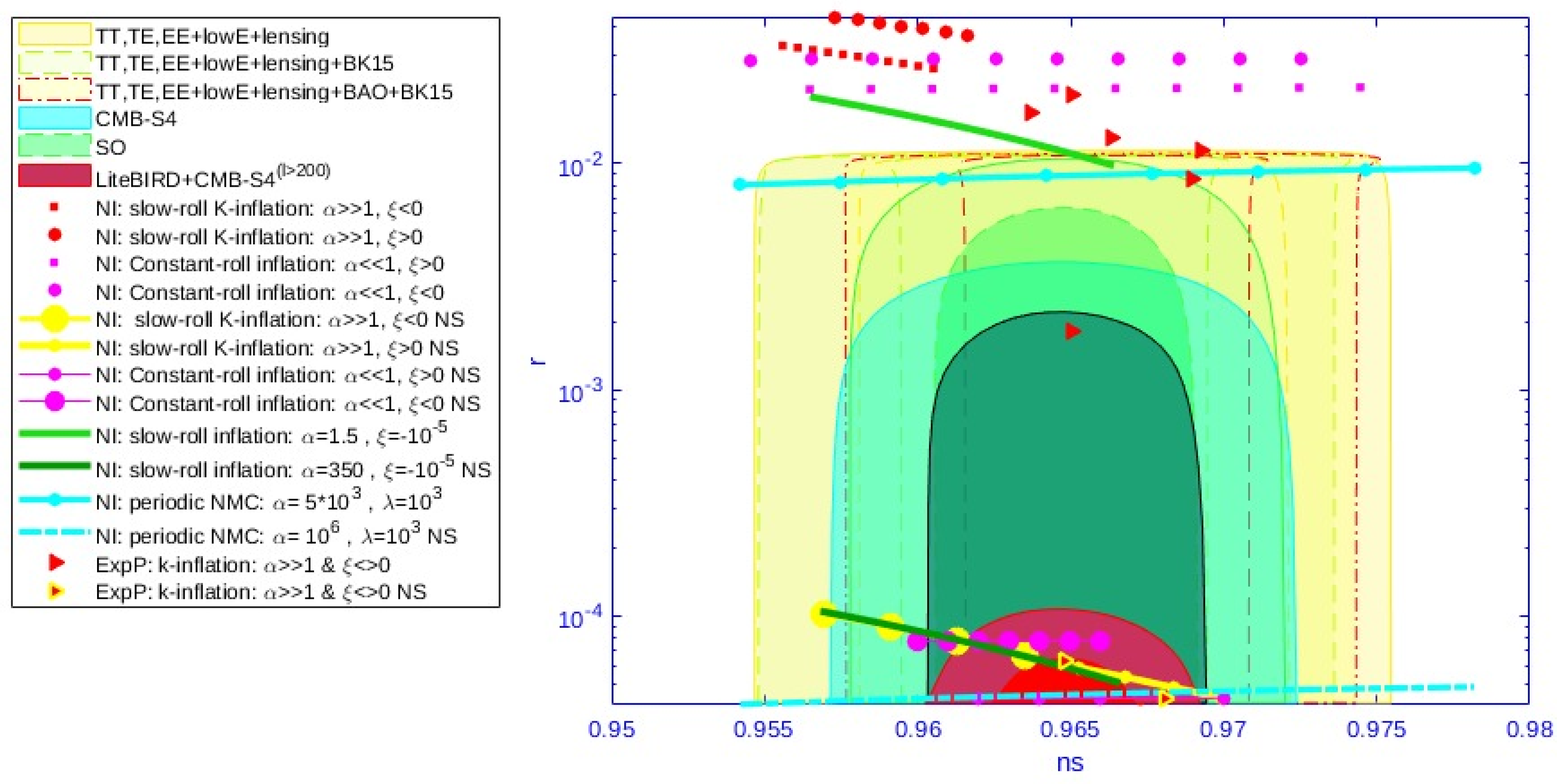
In Figure 1, we reproduce most of the results of refs. [8,9] regarding the cases of Table 2. The exemplified results of Figure 1 were largely in agreement with the observations of Planck 2018 [8,9]. We see, however, that the opposite occurs when Planck 2018 and lensing data alone and their combinations with BICEP2/Keck Array (BK15) and BAO data are taken into account. A large majority of the results are excluded since they do not meet observational constraints. Although adding the results of the ref. [17] makes the theoretical results further away from the observational ones, we do so to illustrate the model’s strength and show its focusing ability. We performed a new scan on the parameters and successfully attained a coincidence with the observational results again, as we can see in Figure 1.

Table 3. The scanned ranges of parameters and the scopes of observables $n_s$ and r for each of the considered cases in Figure 1.

Case	$\mathit{\alpha }$	$\mathit{\xi }/\mathit{\lambda }(\times {10}^{-5})$	${\mathit{V}}_0$	$\mathit{f}/\mathit{\ell }$	${\mathit{n}}_{\mathit{s}}(\times {10}^{-2})$	$\mathit{r}(\times {10}^{-3})$
Limit I, Case I	$1.50$	$-1.00$	$0.24$	$7.00$	$[95.6-96.6]$	$[19.7-979]$
Slow-roll NI	350	$-1.00$	$0.24$	$75.0$	$[95.6-96.6]$	$[0.105-0.05]$
Limit I, Case II	$5\times {10}^3$	1000	1000	1000	$[97.8-95.4]$	$[9.53-8.03]$
Slow-roll NI	$1\times {10}^6$	1000	1000	1000	$[97.8-95.4]$	$[0.049-0.041]$
Limit II, Case I	250	$[90-1.5]$	$0.0002$	$45.0$	$[95.7-96.2]$	$[44.5-36.8]$
K-inflation NI	21,000	$[4.9-5.2]$	$0.006$	$45.0$	$[96.5-97.0]$	$[0.059-0.043]$
Limit II, Case III	500	$z=0.505$		$[1.24-1.44]$	$[97.1-96.4]$	$[1.68-61.1]$
K-inflation ExP	$30,000$	$z=0.505$		$[1.30-1.40]$	$[96.8-96.5]$	$[0.043-0.064]$
Limit III, Case I	$1\times {10}^{-5}$	10	$11.0$	$9.00$	$[96.8-95.4]$	$[29.1-28.7]$
Constant-roll NI	$1\times {10}^{-5}$	10	$2.00$	$9.00$	$[96.6-96.0]$	$[0.078-0.077]$

clarifies the scanned ranges of parameters and the scopes of observables $n_s$ and r for each of the considered cases.

5. Discussion and Conclusions

In this work, we studied the single-field inflationary models within the palatini quadratic gravity with non-minimal coupling between the inflaton field and the gravitational background. Two specific inflationary models are considered and investigated in the study: natural inflation inspired by particle physics and exponential potential model inspired by VLS. In addition, the study assumed different well-motivated functions of non-minimal coupling to gravity.

The study shows an interesting impact of the considered extended gravitational model on the inflationary scenario, where the gravitational model exhibits a focusing effect regarding the observable quantities exemplified as $n_s$ and r. We scanned the parameter spaces of the models in order to compare their results with the observational ones represented by Planck 2018 and BICEP2/Keck Array. To investigate the focusing effect of the model on a more profound level, we include the work with a prediction study about the future expected values of the observables, and we show that the gravitational model, by its focusing ability, succeeded in accommodating the new challenging constraints.

References

- Guth, A.H. The Inflationary Universe: A Possible Solution to the Horizon and Flatness Problems. Phys. Rev. D 1981, 23, 347–356. [Google Scholar] [CrossRef]
- Sotiriou, T.P.; Faraoni, V. Unified cosmic history in modified gravity: From F (R) theory to Lorentz non-invariant models. Rev. Mod. Phys. 2010, 82, 451–497. [Google Scholar] [CrossRef]
- Nojiri, S.; Odintsov, S.D. Unified cosmic history in modified gravity: From F(R) theory to Lorentz non-invariant models. Phys. Rept. 2011, 505, 59–144. [Google Scholar] [CrossRef]
- Nojiri, S.; Odintsov, S.D.; Oikonomou, V.K. Modified Gravity Theories on a Nutshell: Inflation, Bounce and Late-time Evolution. Phys. Rept. 2017, 692, 1–104. [Google Scholar] [CrossRef]
- Myrzakulov, R.; Sebastiani, L.; Vagnozzi, S. Inflation in f(R,ϕ) -theories and mimetic gravity scenario. Eur. Phys. J. C 2015, 75, 444. [Google Scholar] [CrossRef]
- Enckell, V.M.; Enqvist, K.; Rasanen, S.; Wahlman, L.P. Inflation with R2 term in the Palatini formalism. JCAP 2019, 2, 022. [Google Scholar] [CrossRef]
- Ade, P.A.; Ahmed, Z.; Amiri, M.; Barkats, D.; Thakur, R.B.; Bischoff, C.A.; Beck, D.; Bock, J.J.; Boenish, H.; Bullock, E.; et al. Improved Constraints on Primordial Gravitational Waves using Planck, WMAP, and BICEP/Keck Observations through the 2018 Observing Season. Phys. Rev. Lett. 2021, 127, 151301. [Google Scholar] [CrossRef] [PubMed]
- AlHallak, M.; AlRakik, A.; Chamoun, N.; El-Daher, M.S. Palatini f(R) Gravity and Variants of k-/Constant Roll/Warm Inflation within Variation of Strong Coupling Scenario. Universe 2022, 8, 126. [Google Scholar] [CrossRef]
- AlHallak, M.; Chamoun, N.; Eldaher, M.S. Natural Inflation with non minimal coupling to gravity in R2 gravity under the Palatini formalism. JCAP 2022, 10, 001. [Google Scholar] [CrossRef]
- Freese, K.; Frieman, J.A.; Olinto, A.V. Natural inflation with pseudo—Nambu-Goldstone bosons. Phys. Rev. Lett. 1990, 65, 3233–3236. [Google Scholar] [CrossRef] [PubMed]
- Chernikov, N.A.; Tagirov, E.A. Quantum theory of scalar field in de Sitter space-time. In Annales de l’IHP Physique Théorique; Joint Inst. for Nuclear Research: Dubna, Russia, 1968; pp. 109–141, Section A, Tome 9. [Google Scholar]
- Reyimuaji, Y.; Zhang, X. Natural inflation with a nonminimal coupling to gravity. JCAP 2021, 3, 059. [Google Scholar] [CrossRef]
- Ferreira, R.Z.; Notari, A.; Simeon, G. Natural Inflation with a periodic non-minimal coupling. JCAP 2018, 11, 021. [Google Scholar] [CrossRef]
- AlHallak, M.; Chamoun, N. Realization of Power-Law Inflation & Variants via Variation of the Strong Coupling Constant. JCAP 2016, 9, 006. [Google Scholar] [CrossRef]
- Chamoun, N.; Landau, S.J.; Vucetich, H. On Inflation and Variation of the Strong Coupling Constant. Int. J. Mod. Phys. D 2007, 16, 1043–1052. [Google Scholar] [CrossRef]
- AlHallak, M.; Rakik, A.A.; Bitar, S.; Chamoun, N.; Eldaher, M.S. Inflation by variation of the strong coupling constant: Update for Planck 2018. Int. J. Mod. Phys. A 2021, 36, 2150226. [Google Scholar] [CrossRef]
- Bahr-Kalus, B.; Parkinson, D.; Easther, R. Constraining Cosmic Inflation with Observations: Prospects for 2030. arXiv 2022, arXiv:2212.04115. [Google Scholar] [CrossRef]
Figure 1.
A plot of tensor-to-scalar ratio r and spectral index for various cases of Table 2, within limits I, II, and III. the theoretical results of different cases and limitations are compared to the joint 68 and 95% CL regions for , and r, obtained from Planck 2018 and lensing data alone, and their combinations with BICEP2/Keck Array (BK15) and BAO data, in addition to a forecast posterior contours of the CMB experiments (Simons Observatory, CMB-S4, and LiteBIRD) considered in ref. [17]. NI, ExP, and NS stand for Natural inflation, Exponential Potential, and New Scan, respectively.