Proceeding Paper

LRS Bianchi-I Transit Cosmological Models in f(R,T) Gravity †

by
Siwaphiwe Jokweni
1,
Vijay Singh
2,
Aroonkumar Beesham
1,3,4,* and
Binaya Kumar Bishi
1,5
1
Department of Mathematical Sciences, University of Zululand, Kwa-Dlangezwa 3886, South Africa
2
Department of Mathematics, Kirori Mal College, University of Delhi, Delhi 110007, India
3
Faculty of Natural Sciences, Mangosuthu University of Technology, Jacobs 4026, South Africa
4
National Institute for Theoretical and Computational Sciences (NITheCS), Stellenbosch 7611, South Africa
5
Department of Mathematics, Lovely Professional University, Phagwara 144401, India
*
Author to whom correspondence should be addressed.
Presented at the 2nd Electronic Conference on Universe, 16 February–2 March 2023; Available online: https://ecu2023.sciforum.net/.
Phys. Sci. Forum 2023, 7(1), 34; https://doi.org/10.3390/ECU2023-14062
Published: 18 February 2023
(This article belongs to the Proceedings of The 2nd Electronic Conference on Universe)

Abstract

:
A locally rotationally symmetric Bianchi-I model is explored both in general relativity and in f(R,T) gravity, where R is the Ricci scalar and T is the trace of the energy-momentum tensor. Solutions have been found by means of a special Hubble parameter, yielding a hyperbolic hybrid scale factor. Some geometrical parameters have been studied. A comparison is made between solutions in general relativity and in f(R,T) gravity, where in both the theories, the models exhibit rich behaviour from stiff matter to quintessence, phantom, then later mimicking the cosmological constant, depending on some parameters.

1. Introduction

Observational data from refs. [1,2,3] suggest that the universe is currently in an accelerating epoch. A plethora of attempts have been made to explain this phenomenon, but neither of them is compelling. The first attempt is dark energy (DE), which is the hypothesis of exotic matter with the unique feature of anti-gravity due to highly negative pressure which hence accelerates the expansion of the universe [4]. On the other hand, there is insufficient information about DE from the ΛCDM model in general relativity (GR). The cosmological constant (CC) is the primary candidate for DE and the second candidate is modified gravity. The shortcomings [5] of the ΛCDM model enable authors to consider other alternatives to fundamental theories of astrophysics and cosmology. These include the dynamical candidates of DE and modified theories of gravity, e.g., higher derivative theories, Gauss-Bonnet f(G) gravity, f(R) theory, f(T) and f(R,T) gravity theory. Harko et al. [6] introduced f(R,T) gravity, where f(R,T) is an arbitrary function of the Ricci scalar R, and the trace T of the energy-momentum tensor.
Over the years, cosmologists have solved the field equations by means of assuming some cosmological parameters, i.e., Hubble parameter, scale factor, and even some form of deceleration parameter, based on the current understanding in cosmology that the universe has undergone stages of evolution, i.e., inflation, radiation, matter, and late time acceleration. Based on that, the notion of varying deceleration parameter, which changes the signature from deceleration to acceleration, has been applied to many cosmological models. In ref. [7], the authors developed a hyperbolic scale factor. This form of scale factor has attracted a lot of attention over the years, where it was applied for both homogeneous and isotropic or anisotropic space-times through various contexts in cosmology, i.e., see ref. [8]. Recently, the Bianchi-I model with a perfect fluid with various cases of cosmological constant was considered [7].

2. The Formalism of the Model in f(R,T) Gravity

The general action of f (R,T) gravity with units in which 8 π G = c = 1 is given by ref. [6].
S = 1 2 f R , T + 2 L m g d 4 x
We consider   f R ,   T = R + 2 f T , and get the following field equations
R i j 1 2 R g i j = T i j 2 T i j + p g i j f T + f T g i j
where a prime represents an ordinary derivative of f(T) with respect to T. In this work we have chosen f T = λ T , i.e., f R ,   T = R + 2 λ T . The energy-momentum tensor (EMT) of a perfect fluid is T i j = ρ + p u i u j p g i j with ρ and p the energy density and thermodynamic pressure, respectively. The trace of the energy-momentum tensor is T = ρ 3 p . Equation (8) yields
R i j 1 2 R g i j = 1 + 2 λ T i j + λ ρ p g i j .
In this work, we have considered the LRS Bianchi-I spacetime:
d s 2 = d t 2 A 2 t d x 2 B 2 t [ d y 2 + d z 2 ] ,
where A and B are the scale factors and functions of cosmic time t . The average scale factor for the metric (16) is defined as
a = A B 2 1 3
The average Hubble parameter is given by
H = 1 3 A ˙ A + 2 B ˙ B ,
where a dot denotes the derivative with respect to t .
It is crucial to mention that the coupling between geometry and matter in f (R,T) gravity adds some additional terms visible on the RHS of the field equations. These terms must be treated as matter that can be called “coupled matter”. Therefore, to distinguish between the main matter and coupled matter, we replace p with p M and ρ with ρ M   which represents the primary or main matter.
Using the line element (4) and the energy-momentum tensor (EMT) of a perfect fluid, the field Equation (3), yield
B ˙ B 2 + 2 A ˙ A B ˙ B = 1 + 3 λ ρ M λ p M ,
B ˙ B 2 + 2 B ¨ B = 1 + 3 λ p M + λ ρ M ,
A ¨ A + B ¨ B + A ˙ A B ˙ B = 1 + 3 λ p M + λ ρ M .
These equations consist of four unknowns, namely, A ,   B ,   p M ,   ρ M . Therefore, to find exact solutions, one supplementary constraint is required. We assume the following relationship between the Hubble parameter and cosmic time [7]:
H t = m + n C o t h t ,
where m ,   n are positive constants.
On solving, Equation (10) gives
a t = e m t S i n h t n ,
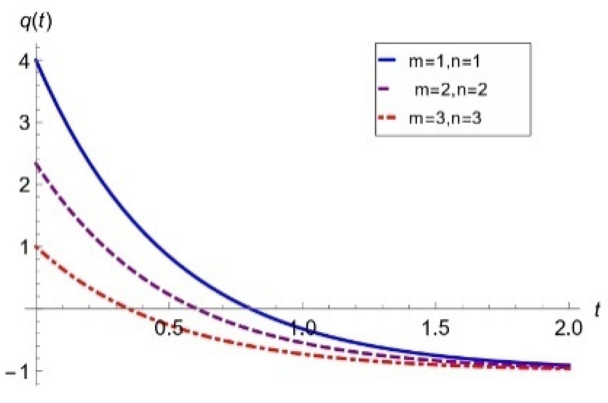
Then, the deceleration parameter q is given by
q = 1 + n m   S i n h t + n   C o s h t 2 ,
and is illustrated in Figure 1.
To eschew repetition,   H t ,     a t ,     q t have been articulated in ref. [7]. The energy density and pressure are given by
ρ = 3 m 2 1 + 4 λ Q 2 3 1 + 2 λ e 6 m t S i n h t 6 n + 3 m 2 C s c h t 2 C o s h t 2 1 + 4 λ + 3 m n C s c h t 2 S i n h 2 t 1 + 4 λ + 2 λ C s c h t 2 1 + 2 λ 1 + 4 λ ,
p = 3 m 2 1 + 4 λ Q 2 3 1 + 2 λ e 6 m t S i n h t 6 n 3 m 2 C s c h t 2 C o s h t 2 1 + 4 λ 3 m n C s c h t 2 S i n h 2 t 1 + 4 λ + 2 m C s c h t 2 1 + 3 λ 1 + 2 λ 1 + 4 λ ,
where Q is a constant of integration.
For a physically realistic cosmological model, the density ρ M must be positive. Unfortunately, at early times, we find that the density ρ M is negative. We shall comment on this later. The pressure is negative throughout the evolution. The equation of state parameter (EoS), ω M = p M / ρ M , is given by:
ω = 3 m 2 1 + 4 λ Q 2 3 1 + 2 λ e 6 m t S i n h t 6 n 3 m 2 C s c h t 2 C o s h t 2 1 + 4 λ 3 m n C s c h t 2 S i n h 2 t 1 + 4 λ + 2 m C s c h t 2 1 + 3 λ 1 + 2 λ 1 + 4 λ 3 m 2 1 + 4 λ Q 2 3 1 + 2 λ e 6 m t S i n h t 6 n + 3 m 2 C s c h t 2 C o s h t 2 1 + 4 λ + 3 m n C s c h t 2 S i n h 2 t 1 + 4 λ + 2 λ C s c h t 2 1 + 2 λ 1 + 4 λ .

2.1. The Behavior of Coupled Matter

As elucidated above, ρ m   and p m do not represent the effective matter in this model. The terms containing λ in the Equations (7)–(9) can be assumed to be associated with the coupled matter. By separating these terms, the equations can be expressed as
B ˙ B 2 + 2 A ˙ A B ˙ B = ρ M + ρ f ,
B ˙ B 2 + 2 B ¨ B = p M + p f ,
A ¨ A + B ¨ B + A ˙ A B ˙ B = p M + p f ,
where ρ f = λ   3 ρ M p M and p f = λ 3 p M ρ M , respectively, represents the energy density and pressure of the coupled matter, and are obtained as
ρ f = 12 λ m 2 1 + 4 λ + 2 λ Q 2 3 1 + 2 λ e 6 m t S i n h t 6 n + 12 λ m 2 C s c h t 2 C o s h t 2 1 + 4 λ + 12 λ m n C s c h t 2 S i n h 2 t 1 + 4 λ 2 m λ C s c h t 2 1 + 2 λ 1 + 4 λ ,
p f = 12 λ m 2 1 + 4 λ 2 λ Q 2 3 1 + 2 λ e 6 m t S i n h t 6 n 12 λ m 2 C s c h t 2 C o s h t 2 1 + 4 λ 12 λ m n C s c h t 2 S i n h 2 t 1 + 4 λ + 2 m λ C s c h t 2 1 + 2 λ 1 + 4 λ .
The EOS for the coupled matter is:
ω f = 12 λ m 2 1 + 4 λ 2 λ Q 2 3 1 + 2 λ e 6 m t S i n h t 6 n 12 λ m 2 C s c h t 2 C o s h t 2 1 + 4 λ 12 λ m n C s c h t 2 S i n h 2 t 1 + 4 λ + 2 m λ C s c h t 2 1 + 2 λ 1 + 4 λ 12 λ m 2 1 + 4 λ + 2 λ Q 2 3 1 + 2 λ e 6 m t S i n h t 6 n + 12 λ m 2 C s c h t 2 C o s h t 2 1 + 4 λ + 12 λ m n C s c h t 2 S i n h 2 t 1 + 4 λ 2 m λ C s c h t 2 1 + 2 λ 1 + 4 λ .

2.2. State-Finder Parameter, Energy Conditions and Stability

2.2.1. State-Finder Analysis

The state finder pair {r, s} allows the examining the features of DE for the model, and to compare with the ΛCDM model. They rely on the third derivative of the scale factor, as they were introduced in ref. [9]. In this model, they are given by
r = a a H 2 = 3 m n + m 2 + n 2 3 n + 3 m 2 C o t h t + 3 m n n 1 C o t h t 2 + n 2 3 n + n 2 C o t h t 3 m + n C o t h t 3 ,
s = r 1 3 q 1 2 = 4 n 3 m + 2 C o t h t 3 m + n C o t h t 3 n 2 3 m 2 4 n + 3 n 2 + m 2 C o s h 2 t + 6 m n S i n h 2 t .
We observe from the above that as t 0 , {r, s} → {0, 0.6}, and as t , {r, s} → {1, 0}. In this model, initially, we have r < 1 and s > 0 , which imply quintessence and phantom, respectively. At late times, the model mimics the ΛCDM model.

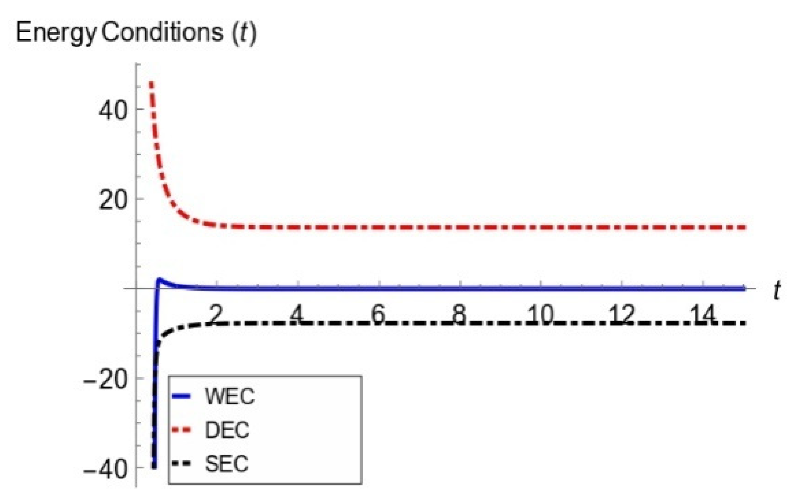
2.2.2. Energy Conditions

The behaviour of the energy conditions such as the Weak Energy Condition (WEC: ρ m   0 ,   ρ m   + p m   0 ), Dominant Energy Condition (DEC: ρ m   p m ) and Strong Energy Condition (SEC: ρ m   + p m 0 ,   ρ m   + 3 p m 0 ), have been studied. They are illustrated in Figure 2.

2.2.3. Stability of the Models through the Speed of Sound

It is crucial to study the stability of the theory, and here, we make use of the technique of speed of sound to study stability [10]. Numerous other techniques can be used to understand the stability of the solutions/methods [11]. The speed of sound is given by v s 2 = d p d ρ . If v s 2 < 0   or v s 2 > 1 , the system is unstable, whereas if 0 v s 2 = d p d ρ 1 , the system is stable. In this model
v s 2 = 378 3 + 3 C o t h t + 3 C o t h t 2 2106 e 18 t C s c h t 18 1 + C o t h t 18 C o t h t C s c h t 2 20 + 63 C o s h t 2 + S i n h 2 t 36 126 3 + 3 C o t h t + 3 C o t h t 2 + 351 e 18 t C s c h t 18 1 + C o t h t 3 C o t h t C s c h t 2 1 + 126 C o s h t 2 + S i n h 2 t
We find that for the values (m = 1, n = 1, Q =1, λ = 1 ), (m = 2, n = 2, Q =2, λ = 2 ), (m = 3, n = 3, Q =3, λ = 3 ), our model is stable (during the early phase of the model), whereas, at present, it is unstable. This is illustrated in Figure 3.

3. Discussion

We have studied an LRS Bianchi I model with a special Hubble parameter H = m + n   C o t h t , yielding q = 1 + n m S i n h t + n C o s h t 2 , where m , n are positive constants. We find that the model transits from early deceleration ( q = 1 + 1 n > 0 for 1 < n < 0 ) to late time acceleration t ,     q = 1 which is in line with observations [1,2,3]. In any physically realistic cosmological model, the energy density ( ρ M ,     ρ f ) ought to be positive throughout the evolution. Here, we observe that for ( m , n , Q , λ > 0 ) initially, both densities are negative but later positive. Due to the complicated nature of the expressions, we have not checked the density for all values of the parameters. Therefore, it is quite possible that the density could be positive for some parameters, and we are investigating this further, and hope to report elsewhere. However, our results do indicate that models have to be checked very carefully to ensure that all reasonable conditions are met. The pressure is negative, which is associated with late-time acceleration.
The DEC is satisfied, but not the SEC. Again, this is in keeping with the late-time acceleration of the model (Figure 2). The other important aspect of the model is for λ = 0 , the solutions of GR are recovered. The effective matter behaves like in f (R,T) gravity due to similar metric potentials in both theories. We can conclude that the model accelerates at late times in f (R,T).
The material presented here is brief, and an extended version will be presented elsewhere.

Author Contributions

Conceptualization, S.J., V.S. and A.B.; methodology, V.S., S.J.; software, S.J.; validation, S.J., A.B. and B.K.B.; formal analysis, S.J.; investigation, S.J.; resources, B.K.B.; data curation, A.B.; writing—original draft preparation, S.J.; writing—review and editing, A.B.; visualization, S.J.; supervision, A.B.; project administration, A.B.; funding acquisition, A.B. All authors have read and agreed to the published version of the manuscript.

Funding

This work is based on research supported wholly/in part by the National Research Foundation of South Africa (NRF), grant numbers (118511).

Institutional Review Board Statement

Not applicable.

Informed Consent Statement

Not applicable.

Data Availability Statement

Not applicable.

Acknowledgments

We thank the reviewers for their valuable comments which led to an improvement in the paper.

Conflicts of Interest

The authors declare no conflict of interest. The funders had no role in the design of the study; in the collection, analyses, or interpretation of data; in the writing of the manuscript, or in the decision to publish the results.

References

  1. Perlmutter, S.; Aldering, G.; Goldhaber, G.; Knop, R.A.; Nugent, P.G.; Castro, P.G.; Deustua, S.; Fabbro, S.; Goobar, A.; Groom, D.E.; et al. Measurements of Ω and Λ from 42 High-Redshift Supernovae. Astrophys. J. 1999, 517, 565–586. [Google Scholar] [CrossRef]
  2. Riess, A.G.; Filippenko, A.V.; Challis, P.; Clocchiatti, A.; Diercks, A.; Garnavich, P.M.; Gilliland, R.L.; Hogan, C.J.; Jha, S.; Kirshner, R.P.; et al. Observational Evidence from Supernovae for an Accelerating Universe and a Cosmological Constant. Astron. J. 1998, 116, 1009–1038. [Google Scholar] [CrossRef]
  3. Allen, S.W.; Schmidt, R.W.; Ebeling, H.; Fabian, A.C.; Van Speybroeck, L. Constraints on dark energy from Chandra observations of the largest relaxed clusters. Mon. Not. R. Astron. Soc. 2004, 353, 457. [Google Scholar] [CrossRef]
  4. Copeland, E.J.; Sami, M.; Tsijikawa, S. Dynamics of dark energy. Int. J. Mod. Phys. D 2006, 15, 1753. [Google Scholar] [CrossRef]
  5. Zlatev, I.; Wang, L.; Steinhardt, P.J. Quintessence, cosmic coincidence, and the cosmological constant. Phys. Rev. Lett. 2008, 82, 896. [Google Scholar] [CrossRef]
  6. Harko, T.; Lobo, F.S.N.; Nojiri, S.; Odintsov, S.D. f(R,T) gravity. Phys. Rev. D 2011, 84, 24020. [Google Scholar] [CrossRef]
  7. Nagpal, R.; Singh, J.K.; Beesham, A.; Shabani, H. Cosmological aspects of a hyperbolic solution in f(R,T) gravity. Ann. Phys. 2019, 405, 234–255. [Google Scholar] [CrossRef]
  8. Singh, J.P.; Baghel, P.S.; Singh, A. Perfect fluid Bianchi typeI cosmological models with time-dependent cosmological term Lambda. Int. J. Mod. Phys. D 2020, 15, 1850132. [Google Scholar]
  9. Alam, U.; Sahni, V.; Deep Saini, T.; Starobinsky, A.A. Exploring the expanding universe and dark energy using the Statefinder diagnostic. Mon. Not. Royal Astron. Soc. 2003, 344, 1057–1074. [Google Scholar] [CrossRef]
  10. Zhao, G.B.; Xia, J.Q.; Li, M.; Feng, B.; Zhang, X. Perturbations of the quintom models of dark energy and the effects on observations. Phys. Rev. D 2005, 72, 123515. [Google Scholar] [CrossRef]
  11. Sadeghi, J.; Setare, M.R.; Amani, A.R.; Noorbakhsh, S.M. Bouncing universe and reconstructing vector field. Phys. Lett. B. 2010, 685, 229–234. [Google Scholar] [CrossRef]
Figure 1. Deceleration parameter vs time.
Psf 07 00034 g001
Figure 2. Behaviour of energy conditions.
Psf 07 00034 g002
Figure 3. Squared of sound speed against time.
Psf 07 00034 g003
Disclaimer/Publisher’s Note: The statements, opinions and data contained in all publications are solely those of the individual author(s) and contributor(s) and not of MDPI and/or the editor(s). MDPI and/or the editor(s) disclaim responsibility for any injury to people or property resulting from any ideas, methods, instructions or products referred to in the content.

