


SuperNest: Accelerated Nested Sampling Applied to Astrophysics and Cosmology †

1
Astrophysics Group, Cavendish Laboratory, J. J. Thomson Avenue, Cambridge CB3 0HE, UK
2
Kavli Institute for Cosmology, Madingley Road, Cambridge CB3 0HA, UK
3
Queens’ College, University of Cambridge, Silver Street, Cambridge CB3 9ET, UK
4
Gonville & Caius College, University of Cambridge, Trinity Street, Cambridge CB2 1TA, UK
*
Author to whom correspondence should be addressed.
†
Presented at the 41st International Workshop on Bayesian Inference and Maximum Entropy Methods in
Science and Engineering, Paris, France, 18–22 July 2022.
Phys. Sci. Forum 2022, 5(1), 51; https://doi.org/10.3390/psf2022005051
Published: 8 March 2023
(This article belongs to the Proceedings of The 41st International Workshop on Bayesian Inference and Maximum Entropy Methods in Science and Engineering)
Abstract
:We present a method for improving the performance of nested sampling as well as its accuracy. Building on previous work we show that posterior repartitioning may be used to reduce the amount of time nested sampling spends in compressing from prior to posterior if a suitable “proposal” distribution is supplied. We showcase this on a cosmological example with a Gaussian posterior, and release the code as an LGPL licensed, extensible Python package supernest.
Keywords:
Bayesian inference1. Introduction
Nested sampling is a multi-purpose tool invented by John Skilling [1] for simultaneous probabilistic integration of high-dimensional distributions and drawing weighted samples. These are essential tasks for the performance of Bayesian model comparison and parameter estimation [2]. It has become widely used across the physical sciences from astrophysics and cosmology through biochemistry and materials science to high energy physics [3].
The performance of nested sampling algorithms, however, suffer in comparison with alternative posterior samplers such as Metropolis–Hastings [4], in particular, when the latter are provided with a pre-trained proposal distribution and start point. This paper allows an apples-to-apples comparison, by providing a mechanism for accelerating nested sampling using proposal distributions. This is achieved using an extension of the posterior repartitioning techniques developed by Chen et al. [5].
2. Background
2.1. Notation
In this section, we establish notation and recall the key terms in nested sampling and Bayesian inference. A probabilistic inference model with a vector of tunable parameters for data D is specified by likelihood and prior . The two-step challenge of inference is to compute the posterior and evidence . Constructing a representation of the posterior is termed parameter estimation, and evaluating an estimate of the evidence comprises model comparison. The four distributions are linked via Bayes theorem:
where both sides of the equation equal to the joint distribution .
It is useful to define the Kullback-Leibler divergence [6] between the prior and the posterior :
One can understand the properties of the KL divergence as a logarithmic ratio of the volume contained in the prior distribution to the volume contained in the posterior distribution:
When both the prior and posterior are uniform (i.e., constant value where they are non-zero), this relation is exact (one can think of the posterior averaging process in Equation (2) as an information theory inspired “smoothing” for non top-hat distributions).
2.2. Nested Sampling
In this section, we will provide a brief primer on the nested sampling algorithm. For a survey of established nested sampling packages and applications, readers are recommended the Nature primer [3]. We begin by initialising initial “live points” drawn from the prior . Then at each iteration, the lowest likelihood live point is marked “dead” and replaced with a new live point drawn from the prior, that is at a higher likelihood. The compression procedure allows one to estimate the density of states, which given the recorded locations of live and dead points leads to estimates of posterior and evidence with respective errors.
Crucially, the algorithm terminates once the running estimate of the error in the evidence is greater than a set fraction of the total estimated evidence. Thus, the time complexity of nested sampling is:
where is the time complexity of evaluating and is the implementation-specific factor representing the time complexity of replacing a dead point with a live point with a higher likelihood, and is the dominant factor for nested sampling over parameter spaces with many dimensions [3]. For rejection nested sampling (e.g., MultiNest [7]) this factor is exponential in the number of tunable parameters d (with a turnover constant in tens of dimensions), and linear in d for chain-based approaches (e.g., PolyChord [8]). The Kullback–Leibler divergence is linear in the d for parameters that are well constrained, as can be seen from Equation (3) by noticing that volumes in parameter space scale with a power of d.
From Equation (4), it follows that the run time of nested sampling, given a resolution fixed by can be reduced by (i) speeding up the likelihood evaluation; (ii) improving the replacement efficiency; (iii) speeding up the prior to posterior compression. The final approach is the one adopted for the repartitioning techniques in this paper.
The accuracy of the evidence is associated with the accumulated Poisson noise, such that the error in is [1]:
Thus, faster compression leads to better accuracy and precision. For a fixed accuracy , we can adjust , which means , given Equation (4). In precision-normalised cases, reducing the effect of the KL divergence term results in quadratic improvements to the speed of nested sampling. Note that the number of live points can be also adjusted. The minimum number is dictated by the quantity of modes in the multi-modal posterior, and implementation dependent considerations: for example, PolyChord needs to generate enough dead point phantoms for an accurate covariance computation. MultiNest needs at least to compute ellipsoidal decompositions.
2.3. Historical Overview of Acceleration Attempts
One approach to partially achieve this form of speed-up is to perform two passes of nested sampling. First, a low resolution pass (few live points) over the entire original prior volume finds the location of the highest concentration of posterior volume, and an evidence estimate . Next, one constructs a much tighter bounding prior with volume around the largest concentration of the posterior. Trivially:
hence, latter inference over the tighter box will finish faster finding the evidence . With a changed prior, this evidence will not be the same as the original. However, for box-priors we can compensate the volumes geometrically, using the fact that the overall evidence satisfies:
See Anstey et al. [9] for examples of this method’s application in real astronomical cases.
3. Posterior Repartitioning
Nested sampling is unusual amongst Bayesian numerical algorithms, in that it distinguishes between the prior and likelihood . Metropolis–Hastings, and Hamiltonian Monte Carlo, for example, are techniques which are only sensitive; (i.e., the joint or unnormalised posterior) is considered for the purposes of acceptance/rejection. Nested sampling, on the other hand, by “sampling from the prior , subject to a hard likelihood constraint ”, separates the two functions.
Chen et al. [5] pioneered an approach which exploits this split, noting that we have the freedom to define a new prior and likelihood , which providing they obey the relation:
will recover the same posterior and evidence. Conceptually, one can think of this as transferring portions of the likelihood into the prior, or vice versa. A cosmological example of this subtle rearranging of portions of likelihood into prior can be found in many codes which implement nested sampling such as cobaya [10], cosmomc [11,12], MontePython [13] or cosmosis [14] in the manner in which they consider Gaussian priors. Codes can either make the choice to incorporate this as part of the prior (typically as an inverse-error-function-based unit hypercube transformation), or as a density term added to the rest of the log-likelihood calculations.
This rearranging affects the Kullback–Leibler divergence. The difference can be found using a posterior average:
If the final term in Equation (9) is negative, repartitioning provides a mechanism for reducing the time to convergence by transferring a reasonable “guess”: the proposal distribution, from likelihood to prior, reducing the Kullback–Leibler divergence between the prior and the posterior . As we have seen before, this both improves performance and increases precision.
3.1. Example 1: Power Posterior Repartitioning
For , any distribution becomes uniform. If a distribution is not uniform, raising it to a power of serves to sharpen or spread the peaks, depending on whether is greater or smaller than 1, in analogy with the thermodynamic inverse temperature of a Boltzmann distribution [3]. For any given value of , a nested sampling run with likelihood and prior recovers the same posterior samples and evidence as a run with and prior .
Chen et al. [5] considered this in the context of a geophysical example. The original intention behind repartitioning was not to improve performance, but rather as a way of making nested sampling more resilient to over-zealously specified priors (e.g., if a user specifies a Gaussian prior which is narrow and/or distant from the peak of the likelihood). Still, the performance implications are valuable. Substituting Equation (10) into Equation (9) shows that varying will change the time to convergence as:
Whether or not this increases or decreases the speed of nested sampling depends on the choice of and to what extent the sharpened prior overlaps with the posterior. Equation (10) is valid for any choice of , and while any specific choice can be useful, Chen et al. [5] demonstrated that still greater power comes from considering it as an additional parameter to sample over, effectively extending the parameter space to with a prior on . A posterior value of the parameter close to 0 therefore indicates that the prior was poorly chosen, i.e., that there is significant tension between prior and posterior.
One could consider this for the purposes of acceleration by allowing to take a range wider than , for example, by using an exponential prior . There is, however, no need to restrict ourselves to the case of power posterior repartitioning, or indeed to a priors , which are direct transformations of the original .
3.2. Example 0: Replacement Repartitioning
The simplest repartitioning scheme is to simply use a different prior , but compensate for this with the adjusted likelihood:
From Equation (9), we can see that if is close to as quantified by the KL divergence, nested sampling terminates sooner (with in the limiting case ). However, a poorly specified proposal will pessimise the choices of new live points, thus making the problem harder. Indeed, a poorly chosen proposal can prevent us gaining any usable information.
3.3. Example 2: Additive Superpositional Repartitioning
Another repartitioning scheme is to consider an additive superposition of the original prior with another normalised distribution :
Here, does not need to be related to the original prior, and could, for example, be a Gaussian proposal distribution (often supplied with cosmological sampling packages for common likelihood combinations), or a tighter box prior as suggested in Section 2.3.
This scheme can be generalised to superpositions of N alternative distributions . Consider:
However, additive superpositional repartitioning in practice has the issue of poor generalisation to higher dimensions and/or complex priors due to the difficulty of implementing an analytic unit hypercube transformation. Further work is required to fully explore this using nested samplers that do not rely on prior point–percent functions which produce said transformations. We thank Xy Wang for exploring the possibility of these models in the first instance as part of her University of Cambridge master’s dissertation.
4. Supernest: Stochastic Superpositional Repartitioning
The above examples lead us to the proposed repartitioning scheme. Just as with additive repartitioning, we allow, arbitrarily, many unrelated priors to be superimposed. However, we side-step the multivariate point-percent function correction problem by sampling from each of the priors with some probability. We achieve this by adding an integer selection parameter , such that:
and then is sampled over with a discrete (typically uniform) prior . The choice of said prior depends on the confidence in each of the proposals. When applied to nested sampling, at the end of the run, one will recover a (joint) posterior on , which will indicate which proposal was chosen more frequently, as the usual Bayesian balance between the corresponding modified likelihood and KL divergence of the favoured bin.
In the additive case from Section 3.3, the primary difficulty is in obtaining the point-percent function of the repartitioned prior. The more priors are introduced, the harder the calculation. For the stochastic case, the prior of the superposition is the superposition of the individual priors. Thus, if one knows the point percent functions of the constituent priors, simply copying them is the “calculation”.
Additionally, only one of the prior quantile/likelihood pairs is evaluated for each point. Thus, the time complexity of the likelihood evaluation of a superposition of multiple likelihoods is . By contrast, the equivalent time complexity for the additive superposition is the sum of the time complexities: . For comparison, if we fed 100 identical models to the stochastic mixture, we would not see a performance regression, while the additive superposition would take 100 times longer to compute.
5. Cosmological Example
For the purposes of demonstration, we choose a likelihood which is Gaussian in the parameters, with parameter means and parameter covariances as given by the Planck legacy archive chains [15], and prior given by the default prior widths as specified in those chains. This has six cosmological parameters and 21 nuisance parameters associated with galactic foregrounds and satellite calibration, giving 27 parameters to constrain. In its default mode, this therefore gives and , and for this example an . This provides a proxy for a nested sampling problem of interests to cosmologists, whilst being fast enough numerically to explore a variety of configurations.
We run PolyChord wrapped with supernest, both with their default settings. PolyChord, in addition, is set with a precision criterion of , i.e., stopping when the live points contain 10% of the remaining evidence. As a representative example, we first choose a Gaussian proposal with the same covariance as the parameters, inflated by a factor of in volume, and offset by a random vector drawn from the posterior. This gives a proposal which is conservative (much wider than the posterior), and approximately correctly centered.
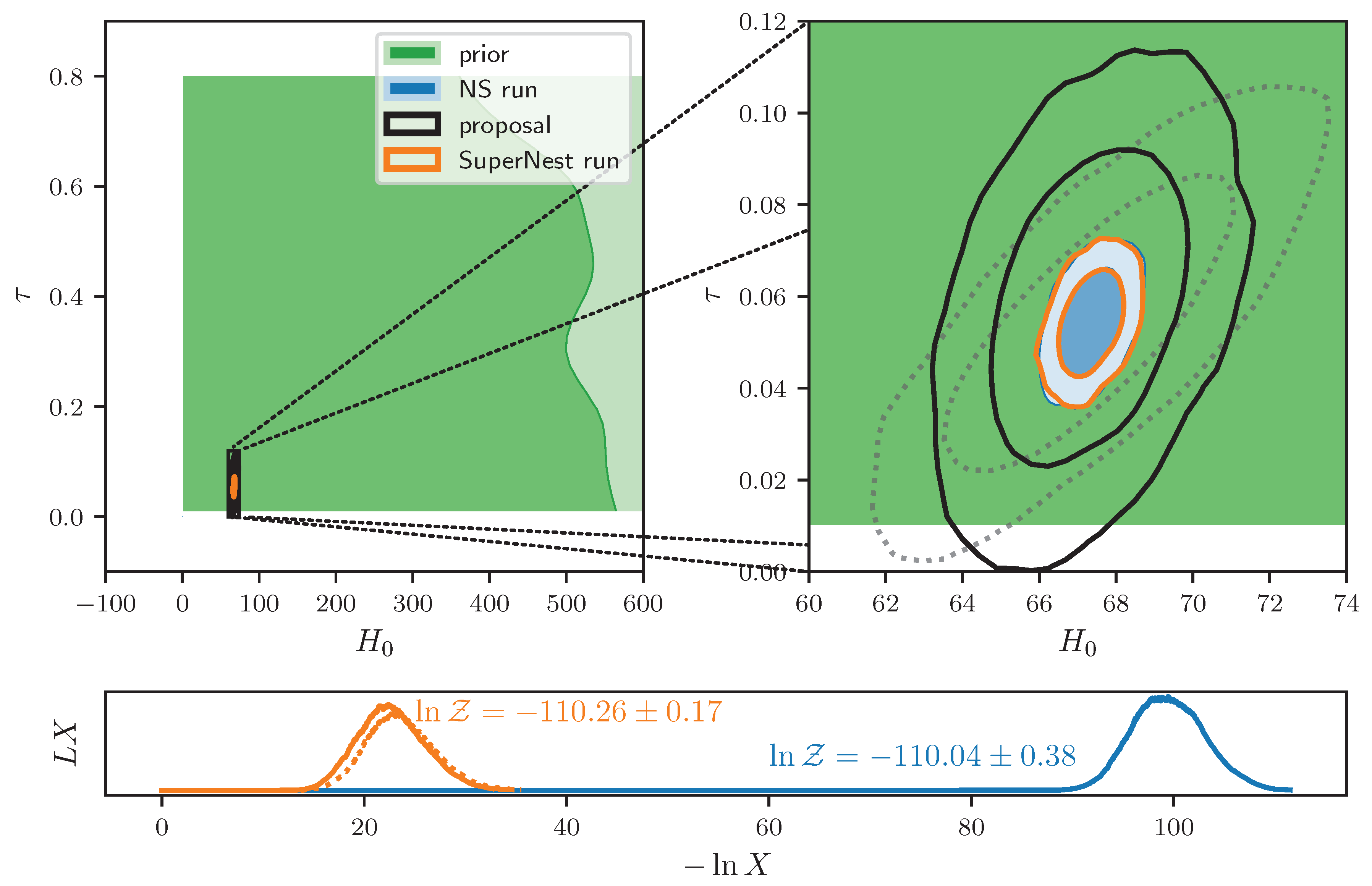
The performance of this example is shown in Figure 1. We can see that the algorithm terminates approximately three times faster, with an error bar that is approximately two times smaller despite the perturbation. Usually to reduce the error bar by a factor of 2, one would need to increase the number of live points by a factor of 4. Thus, when precision-normalised supernest achieved an order-of-magnitude improvement over the traditional nested sampling run. Further improvements to this speed are achievable if a more compact (and possibly larger number of) proposal distributions are used.
As a second example, where the covariance of the proposal does not align with the covariance of the posterior, we draw an inverse Wishart distributed covariance matrix, with degrees of freedom and scale matrix equal to the covariance, once again inflating the result in volume by , and offsetting the result by a random vector drawn from the posterior. The performance is unaffected to within sampling fluctuation, with the recovered evidence equal to within error.
6. Conclusions
We presented a method for improving the performance and accuracy of nested sampling using the recent innovations in posterior repartitioning of Chen et al. [5]. The approach functions by reducing the effective prior-to-posterior compression that nested sampling “sees”, and hence reducing both the runtime and accumulated Poisson error in the evidence estimate. We discussed a variety of alternative posterior repartitioning strategies before settling on a stochastic superpositional scheme, and demonstrated that on a cosmological example even conservative proposals have the capacity to speed up nested sampling runs by an order of magnitude.
This performance improvement is achieved by trimming off the long prior-to-posterior compression phase seen in the blue but not orange curve of the lower panel of Figure 1. The remaining majority of the time is spent in traversing the typical set. Accelerating the pace at which nested sampling does this is a matter of ongoing research.
This work will be followed by a re-examination of the repartitioning, in particular, by considering more general cases than the ones considered here. In a follow up study we shall provide a more mathematical look into how further performance improvements can be achieved via modifications to nested samplers, hysteretic priors on the choice parameter, as well as exploring the connection between prior spaces and Hilbert spaces. Finally, we shall consider a reformulation of Bayesian methods using functionals, and explore the implications of consistent partitioning (a generalisation of posterior repartitioning) applied to Bayesian inference in functional space.
Author Contributions
Conceptualization, A.P. and W.H.; methodology A.P.; software, A.P.; validation, A.P. and W.H.; formal analysis A.P. and W.H.; investigation A.P.; resources W.H.; data curation A.P. and W.H.; writing—original draft preparation A.P.; writing—review and editing W.H.; visualization A.P. and W.H.; supervision W.H.; project demonstration A.P.; funding acquisition W.H. All authors have read and agreed to the published version of the manuscript.
Funding
This research received no external funding.
Institutional Review Board Statement
Not applicable.
Informed Consent Statement
Not applicable.
Data Availability Statement
Data is available at https://doi.org/10.5281/zenodo.7703906 or at https://gitlab.com/a-p-petrosyan/sspr/.
Conflicts of Interest
The authors declare no conflict of interest.
References
- Skilling, J. Nested sampling for general Bayesian computation. Bayesian Anal. 2006, 1, 833–859. [Google Scholar] [CrossRef]
- MacKay, D.J.C. Monte-Carlo methods. In Information Theory, Inference, and Learning Algorithms; Cambridge University Press: Cambridge, UK, 2003; Chapter 29; pp. 379–380. [Google Scholar]
- Ashton, G.; Bernstein, N.; Buchner, J.; Chen, X.; Csányi, G.; Fowlie, A.; Feroz, F.; Griffiths, M.; Handley, W.; Habeck, M.; et al. Author Correction: Nested sampling for physical scientists. Nat. Rev. Methods Prim. 2022, 2, 44. [Google Scholar] [CrossRef]
- Arminger, G.; Muthén, B.O. A Bayesian approach to nonlinear latent variable models using the Gibbs sampler and the metropolis-hastings algorithm. Psychometrika 1998, 63, 271–300. [Google Scholar] [CrossRef] [Green Version]
- Chen, X.; Feroz, F.; Hobson, M. Bayesian automated posterior repartitioning for nested sampling. arXiv 2019, arXiv:1908.04655. [Google Scholar]
- Kullback, S.; Leibler, R.A. On Information and Sufficiency. Ann. Math. Stat. 1951, 22, 79–86. [Google Scholar] [CrossRef]
- Feroz, F.; Hobson, M.P.; Bridges, M. MultiNest: An efficient and robust Bayesian inference tool for cosmology and particle physics. Mon. Not. R. Astron. Soc. 2009, 398, 1601–1614. [Google Scholar] [CrossRef] [Green Version]
- Handley, W.J.; Hobson, M.P.; Lasenby, A.N. polychord: Next-generation nested sampling. Mon. Not. R. Astron. Soc. 2015, 453, 4384–4398. [Google Scholar] [CrossRef] [Green Version]
- Anstey, D.; de Lera Acedo, E.; Handley, W. A general Bayesian framework for foreground modelling and chromaticity correction for global 21 cm experiments. Mon. Not. R. Astron. Soc. 2021, 506, 2041–2058. [Google Scholar] [CrossRef]
- Torrado, J.; Lewis, A. Cobaya: Code for Bayesian analysis of hierarchical physical models. J. Cosmol. Astropart. Phys. 2021, 2021, 57. [Google Scholar] [CrossRef]
- Lewis, A.; Bridle, S. Cosmological parameters from CMB and other data: A Monte Carlo approach. Phys. Rev. D 2002, 66, 103511. [Google Scholar] [CrossRef] [Green Version]
- Lewis, A. Efficient sampling of fast and slow cosmological parameters. Phys. Rev. D 2013, 87, 103529. [Google Scholar] [CrossRef] [Green Version]
- Brinckmann, T.; Lesgourgues, J. MontePython 3: Boosted MCMC sampler and other features. Phys. Dark Universe 2019, 24, 100260. [Google Scholar] [CrossRef] [Green Version]
- Zuntz, J.; Paterno, M.; Jennings, E.; Rudd, D.; Manzotti, A.; Dodelson, S.; Bridle, S.; Sehrish, S.; Kowalkowski, J. CosmoSIS: Modular cosmological parameter estimation. Astron. Comput. 2015, 12, 45–59. [Google Scholar] [CrossRef] [Green Version]
- Planck Collaboration. Planck 2018 results. VI. Cosmological parameters. Astron. Astrophys. 2020, 641, A6. [Google Scholar] [CrossRef] [Green Version]
- Higson, E.; Handley, W.; Hobson, M.; Lasenby, A.N. Dynamic nested sampling: An improved algorithm for parameter estimation and evidence calculation. Stat. Comput. 2018, 29, 891–913. [Google Scholar] [CrossRef] [Green Version]
Figure 1.
supernest in action. The top panels show the parameter spaces of the Hubble constant and optical depth to reionisation [15] with all other CDM and nuisance parameters marginalised out. Contours show the 66% and 95% credibility regions of the prior (green) and nested sampling posterior (blue), alongside the proposal distribution (black) provided to supernest which recovers the same posterior (orange) as the original NS run. The left hand plot visualised the prior, whilst the right hand plot zooms in on the posterior for clarity. The lower panel shows the Higson plot [16] of the two runs. Here, the evidences recovered are consistent, and the supernest run in orange has a more accurate evidence inference, associated with the fact that the compression in prior volume is substantially lower, meaning the nested sampling run terminates in approximately a third the time. An alternative proposal distribution with dashed lines is also plotted, which recovers an evidence of , consistent to within sampling error.

Disclaimer/Publisher’s Note: The statements, opinions and data contained in all publications are solely those of the individual author(s) and contributor(s) and not of MDPI and/or the editor(s). MDPI and/or the editor(s) disclaim responsibility for any injury to people or property resulting from any ideas, methods, instructions or products referred to in the content. |
© 2023 by the authors. Licensee MDPI, Basel, Switzerland. This article is an open access article distributed under the terms and conditions of the Creative Commons Attribution (CC BY) license (https://creativecommons.org/licenses/by/4.0/).
Share and Cite
MDPI and ACS Style
Petrosyan, A.; Handley, W. SuperNest: Accelerated Nested Sampling Applied to Astrophysics and Cosmology. Phys. Sci. Forum 2022, 5, 51. https://doi.org/10.3390/psf2022005051
AMA Style
Petrosyan A, Handley W. SuperNest: Accelerated Nested Sampling Applied to Astrophysics and Cosmology. Physical Sciences Forum. 2022; 5(1):51. https://doi.org/10.3390/psf2022005051
Chicago/Turabian StylePetrosyan, Aleksandr, and Will Handley. 2022. "SuperNest: Accelerated Nested Sampling Applied to Astrophysics and Cosmology" Physical Sciences Forum 5, no. 1: 51. https://doi.org/10.3390/psf2022005051