Towards Positive Energy Districts: Energy Renovation of a Mediterranean District and Activation of Energy Flexibility ^†

Abstract

The paper presents the analysis of energy retrofitting, integration of renewable energy and activation of energy flexibility in a cluster of buildings in the surroundings of a port on the Mediterranean Sea in Southern Italy, with the aim of checking the potential for it to achieve the status of positive energy district (PED). The objective of this study is to improve the contemporaneity between local energy generation and energy demand and reduce CO_2eq emissions by considering signals that reflect the environmental variability of the electricity grid, through flexibility solutions applied to the HVAC system. The proposed scenarios are based on the dynamic simulation of the district and analyze the effect of actions that activate the energy flexibility of buildings through advanced control strategies of the air conditioning system. The results show that the joint action of energy efficiency strategies, integration of solar energy and energy flexibility improves the environmental sustainability of the district and the balance of energy flows. Specifically, the activation of energy flexibility contributes to a 10% reduction in operational CO_2eq emissions and increases in self-consumption of energy per year. The operational emissions of the district vary from the base value of 33.37 tons CO_2eq/y to 19.52 tons CO_2eq/y in the scenario based on the integration of solar energy systems and energy efficiency measures, and to 17.39 tons CO_2eq/y when also the demand-side energy flexibility is activated.

1. Introduction

Research on development paths oriented towards sustainability and the decarbonisation of technological and energy processes is nowadays at the center of energy and social policies and of the interest of the scientific community. The ecological transition is already underway, but further efforts are needed in order to achieve the climate neutrality objective by 2050, curb climate change [1,2,3] and, overall, comply with the sustainable development goals [4,5]. In this context, the buildings sector requires particular attention considering that it contributes to 39% of CO₂ emissions globally and that cities are destined to become energy innovation hubs, producers of clean energy and laboratories of the concept of sustainable development [6,7]. In this direction, however, distributed energy generation requires further research efforts in the field of management of energy flows inside and outside the urban environment, balancing the electricity grid and optimizing energy systems and the energy behavior of buildings [7,8,9,10]. Indeed, the need for net zero or positive energy buildings is not limited to energy balances but is marking the rise in research and implementation of energy flexibility practices [11,12,13]. Moreover, and as also highlighted in [14,15], the energy efficiency of the building stock (building envelope, energy systems, local energy availability) and its redesign in compliance with local technical constraints, energy performance requirements and the targets of environmental, economic and social sustainability are also crucial.

Energy flexibility in urban environments is an emerging research field that aims to identify smart management solutions of the energy flows aimed at satisfying specific objectives, such as the improvement of contemporaneity between intermittent on-site energy generation (e.g., weather-driven energy sources such as photovoltaic, wind, solar, etc.) and energy demand. The contribution of the activation of energy flexibility in buildings is also fundamental with regard to the recent growing diffusion of positive energy districts (PEDs).

Research on positive energy districts is highly topical thanks to the attention of the scientific community, the International Energy Agency (IEA) and the initiatives and projects financed with the aim of promoting the dissemination of PEDs and favoring the transformation of cities into energy eco-innovation hubs.

1.1. Positive Energy Districts and Energy Flexibility

A positive energy district (PED) could be broadly defined as an innovative urban area, with defined boundaries, characterized by a positive energy balance between local renewable energy generation and energy demand [16,17,18]. The PED concept is related to the climate and sustainability goals and aims to accelerate the transition towards decarbonised cities and a sustainable society.

Among the several initiatives and pilot projects, action no. 3.2 of the European Union Strategic Energy Technology (EU-SET) plan aimed at the realization of 100 PEDs by 2025, based on the development and implementation of smart energy management solutions [19], on the one hand, while the Joint Programming Initiative (JPI) Urban Europe [20,21] works to support the diffusion and economic financing of PED projects in Europe. In addition, the International Energy Agency’s Energy in Buildings and Communities (IEA-EBC) Annex 83 “positive energy districts” focuses on the challenges and needs for conceptualisation, modeling and evaluation to stimulate research on PEDs and guide their planning and operation [17]. Within this framework, energy flexibility is considered a key factor in balancing the energy flows within the PED and in the interaction with the surrounding energy networks.

Along the same line, [22] found that the redesign of existing districts from a PED perspective should be directed towards the combination energy efficiency and energy flexibility strategies in order to obtain a positive balance even in the case of high population density, while [23,24] highlights the need for energy sharing and optimal control in energy communities.

However, as highlighted in [25,26], the need for smart and demand management approaches energy in PEDs requires research efforts to develop and demonstrate energy solutions that incorporate the concept of energy flexibility. On the other hand and as discussed in [27], as a result of the IEA-EBC Annex 67 “Energy Flexible Buildings” and Annex 82 “Energy Flexible Buildings Towards Resilient Low Carbon Energy Systems”, it is necessary to shift the focus from the energy flexibility of the single building to the district one in order to work with aggregate quantities of energy, contribute more to the interaction with the surrounding energy grids and increase flexibility potential.

The general definition of energy flexibility is as follows: “The ability to manage demand and generation according to the local climatic conditions, user needs and grid requirements” [28]. Indeed, strategies for activating energy flexibility in urban environments aim to modify generation and load profiles in response to energy, environmental or economic signals, generally known as penalty signals [28,29].

These penalty signals can be of different types and must be specified on the basis of the characteristics and research objectives for each case study. In general, they could be based on the price of electricity, on CO₂ emissions or specific incentives aimed at reducing the risk of congestion phenomena in the electricity grid, etc. [11,30,31,32].

Energy flexibility approaches fall within the broader concept of demand-side management (DSM), and could cover different areas such as the following: integration of energy storage systems or electric vehicles, adjustment of air-conditioning systems in order to exploit the passive thermal mass of the building envelope, ventilation or domestic hot water (DHW) production control, management of programmable equipment, etc. [27,33,34]. Some literature experiences at the single-building level concerned the application of rule-based control (RBC) or model predictive control (MPC) algorithms for the flexible management of the space heating and cooling set-point and/or DHW production [11,31,35,36,37,38,39,40,41]; some others concerned the integration and RBC flexible control of energy storage systems (TES and/or BESS) [11,42,43,44] or the flexible operation of ground source heat pumps [45], etc.

With regard to the penalty signal that guides the control algorithms, directly linked to the objective of the study, the fact that the penalty signal is mostly of an economic nature emerges, except for some cases in which it instead reflects the environmental characteristics of the electricity grid (carbon footprint of potentially imported energy on an hourly basis) [11,37].

Although there is a great variety of experience with flexibility at the individual building level, research at the district level is limited and needs definition and demonstration of flexibility methods and practices. As discussed in [46], attention to the cluster scale would benefit from the differences in energy consumption patterns between buildings, favouring the flexibility potential. However, [27] highlighted the need for the control of negative co-impacts of flexibility approaches such as higher rebound peaks on the one hand, and of more detailed building models and controls on the other.

In this regard, further research efforts are required in order to elaborate data specific to the district scale, especially in positive energy districts which would benefit from the activation of energy flexibility in balancing flows and reducing emissions and operating costs [47].

The general line of this research is placed in this context, which focuses on the redesign of an existing district in order to turning it into a positive energy district and the demonstration of some energy efficiency and energy flexibility strategies.

1.2. Objective and Structure of the Study

This article summarizes and discusses the key points of a redesign scenario from a PED perspective of an existing cluster of commercial and office buildings located in the Mediterranean area (Licata, Italy). Some scenarios based on the analysis of the energy retrofitting, integration of renewable energy systems and activation of energy flexibility are described in this paper.

The objectives of the research are as follows:

• The quantification of the energy–environmental impacts of the district retrofitting in order to achieve the PED status;
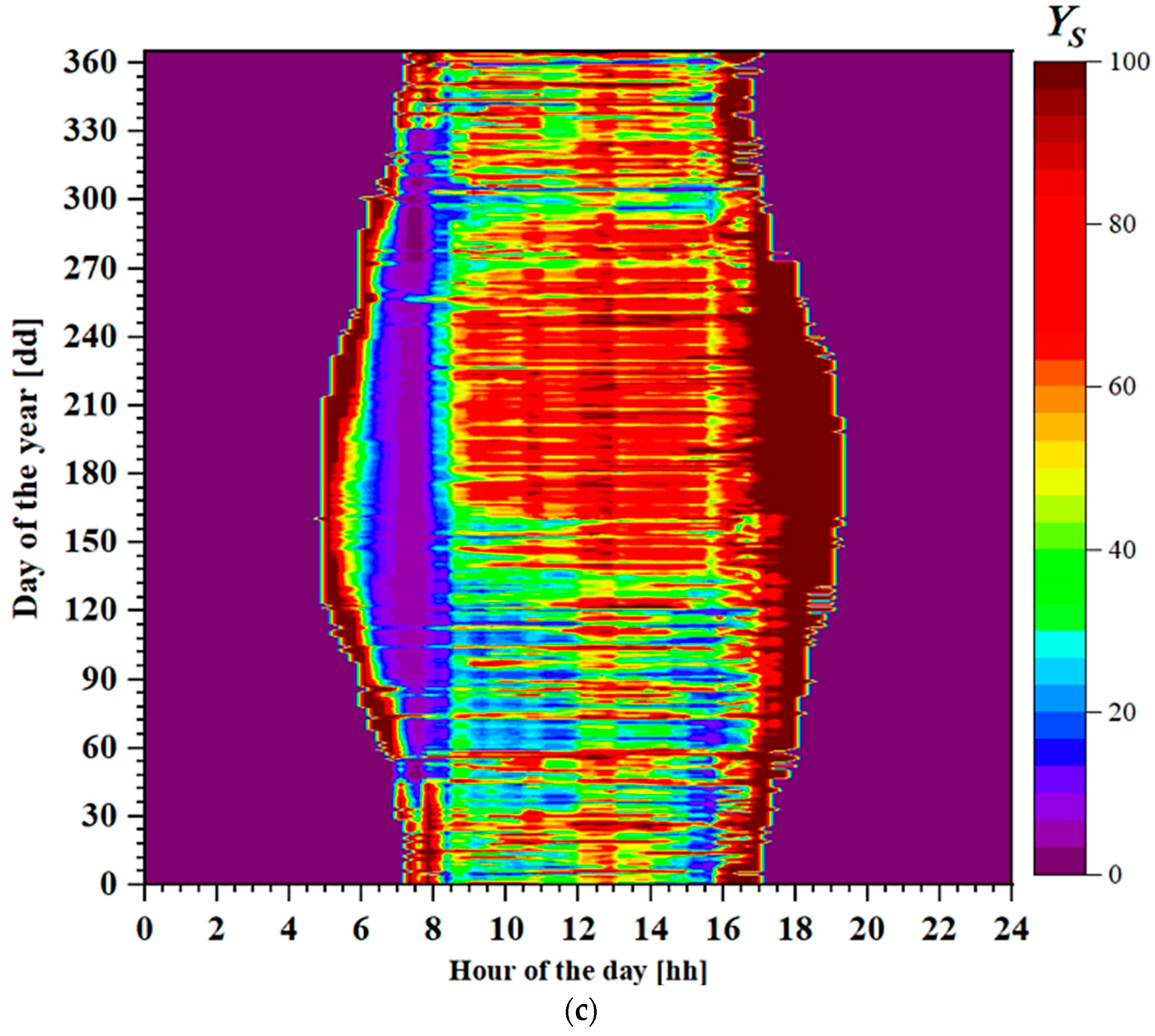
• The investigation of the activation potential of the energy flexibility of the district in terms of interaction with the electricity grid, self-consumption of energy from local RES and reduction in the carbon footprint, considering signals that reflect the environmental variability of the grid, operational costs and reduction in peak loads. In particular, the research work aims at investigating the potential of control algorithms for the air-conditioning system in order to activate the energy flexibility offered by thermal mass of buildings and at evaluating the influence of energy flexibility on the PED energy balance.

This document is structured in four sections. Section 2 contains a description of the case study and illustrates the research methodology adopted for the (a) dynamic analysis of the energy–environmental performance and energy flexibility of the district, (b) redesign of the district in order to achieve the PED target and the development of flexible control algorithms for the management and balancing of energy flows within it, and (c) the analysis of energy, environmental and flexibility impacts through appropriate key performance indicators (KPIs) and calculation methods.

Section 3 shows the research results related to the calibration of the model on the basis of real measured data, analysis of the thermo-physical and energy behavior of the district, analysis of the redesign scenario aimed at the PED target, analysis of the flexibility scenarios, comparison of the results and discussion of the benefits and energy–environmental impacts resulting from the implementation of flexible control.

Finally, Section 4 presents the conclusions of the study and possible future perspectives.

2. Materials and Method

This section contains the description of the case study and illustrates the research methodology followed:

• Develop a model of the district consistent with the real measured data and analyze its behavior in a dynamic simulation regime;
• Evaluate the potential for energy efficiency and integration of renewable energy sources;
• Plan the redesign of the district from a positive energy district perspective;
• Define energy flexibility strategies aimed at managing energy flows in the building cluster;
• Evaluate the impacts in terms of interaction with the electricity grid, self-consumption of energy, energy flexibility and operational CO₂ equivalent (CO_2eq) emissions.

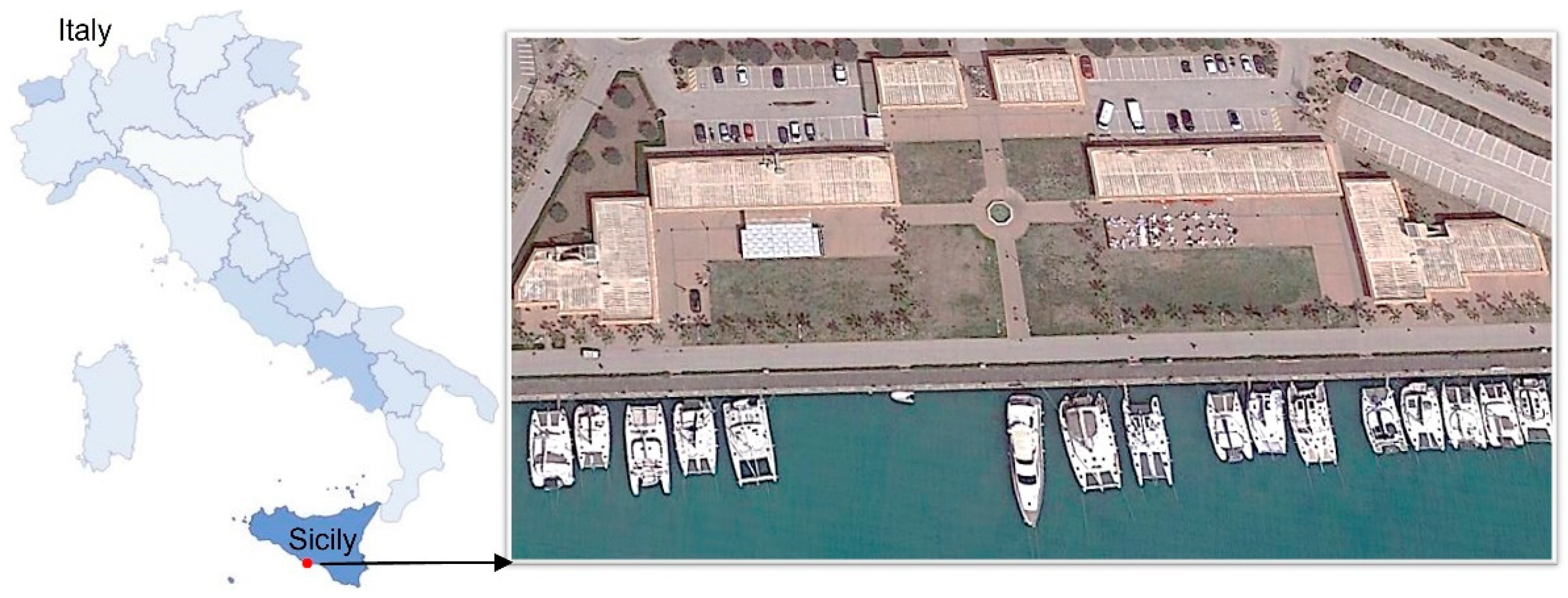
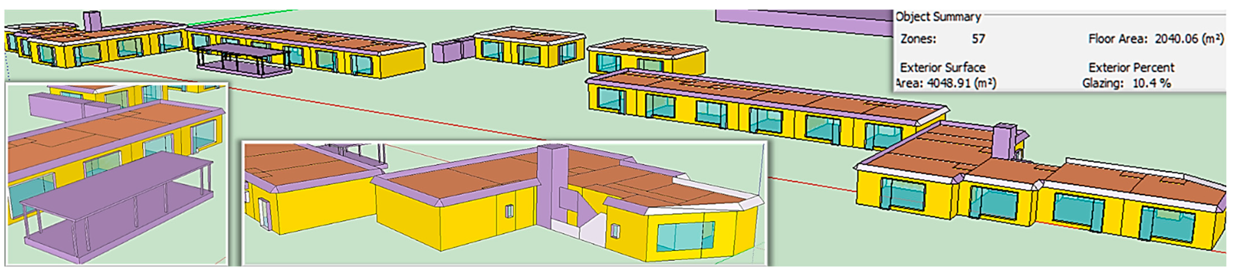
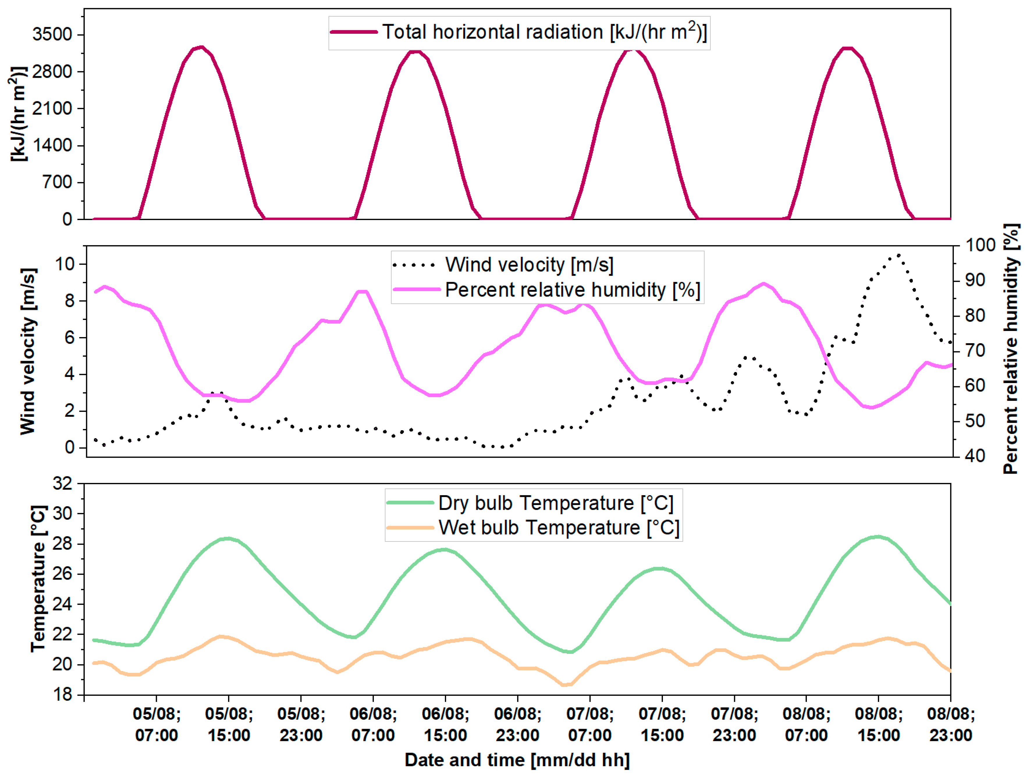
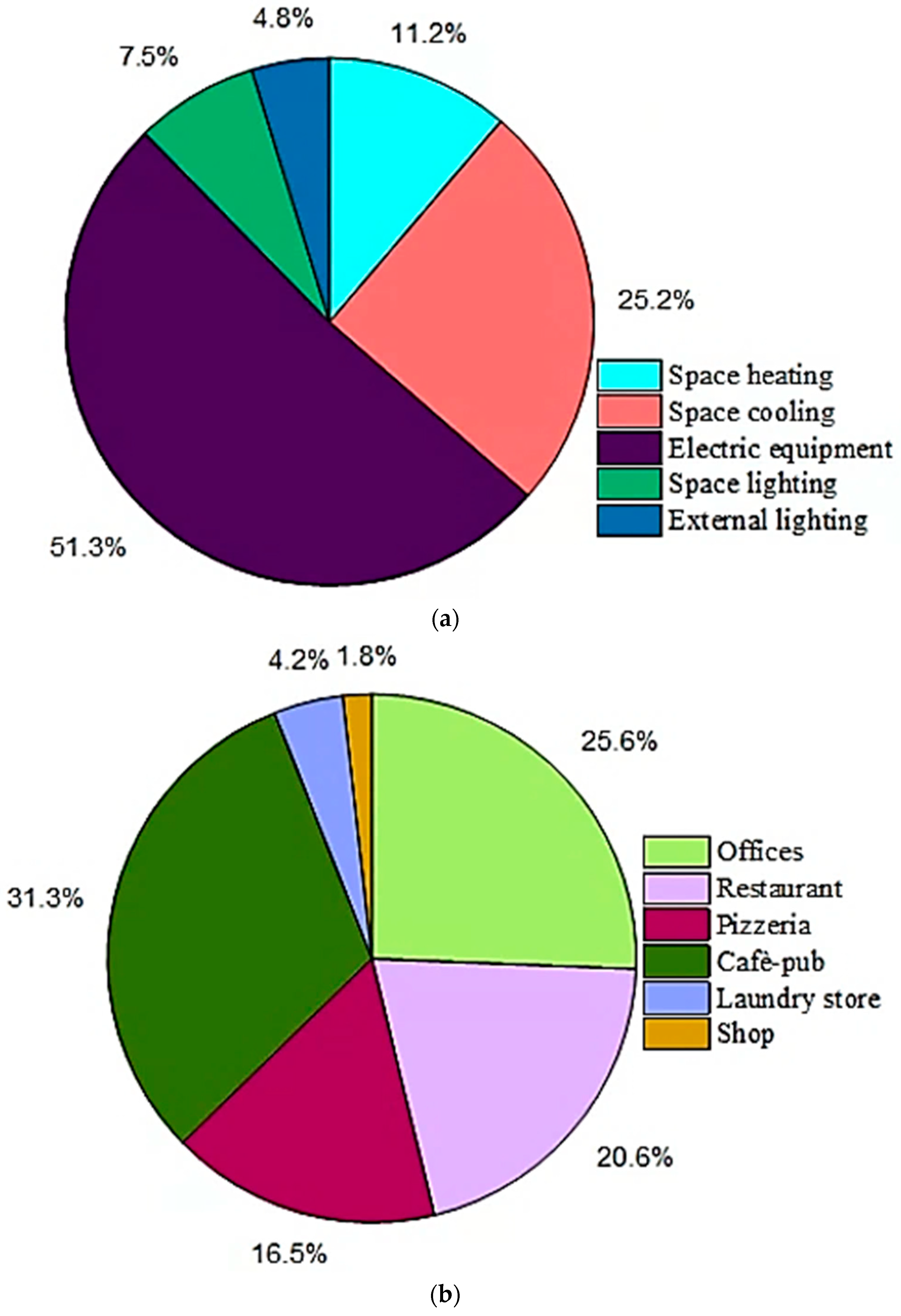
2.1. Description of the Case Study

The case study is a Mediterranean cluster of commercial and office buildings located in the port area of Licata, Sicily, Italy (Figure 1).

During the on site investigation phase, data related to the geometry of the district, occupation and use, installed systems and energy consumption of the buildings were collected. The cluster includes eight offices, a restaurant, a pizzeria, a pub-cafeteria, a laundry, a shop (nautical store) and other unoccupied premises. The total floor area is equal to 2040 m² and the inter-floor height is equal to 3.70 m, while the windows to wall ratio is equal to 10.4%. The building envelope composition is the same between all buildings and therefore have the same layers and transmittance. Specifically, there is no thermal insulation and the transmittance value U [W/(m² K)] is expected to be very close to 0.77 for the external vertical walls, 2.24 for the horizontal external roof, 2 for the interior walls and 1.53 for the ground floor among all buildings. The windows are of the double-glazed type with a gas gap. All buildings are equipped with heat pumps for space air-conditioning and are naturally ventilated.

Table 1. Summary of internal loads per building type and main characteristics of energy systems.

Building Type	Lighting [W/m2]	Equipment [W/m2]	COP [-]	EER [-]
Office building	8.31	20.97	2.8	2.44
Restaurant	6	34.76	3.32	3
Pizzeria	7	262.60	3.41	3.21
Café-Pub	11.12	30.29	3.39	2.95
Laundry store	3.09	327.77	3.41	3.21
Nautical store	2	5.90	3.95	3.5

summarizes the internal loads and the main characteristics of the energy systems per building type.

As for the occupation and use of the buildings, it should be noted the city of Licata presents a variable population depending on the season of year with peaks during the summer months and depopulation during the remaining time of the year. This affects the work rhythms of restaurant and commercial businesses in general, reflected in highly variable energy consumption during the months of the year.

On average, the restaurant is open to the public from 12:30 to 14:30 and 19:30 to 23:00 with extensions of working hours in the summer months and early closure in the winter. The building is also occupied by workers in the time slots 10:30–12:30, 14:30–15:30 and 18:30–19:30.

The kitchen area is usually occupied by two people, while the number of customers occupying the hall varies according to the time of day and the seasons.

The pizzeria building is open during the hours 17:00–24:00 from June to September, while in periods of low population it operates only on Saturdays. Occupancy varies, but on average around three people are present in the kitchen areas.

The café-pub is open on average from 8:30 to 01:00 from June to September. In the other periods of the year, closing is brought forward to 10.00 p.m. on average. The number of occupants in the kitchen area is generally equal to equal, while that of the internal lounge varies with the hours of the day and the months of the year. The building, as well as the restaurant, have an outdoor lounge which is generally occupied in the summer months.

The laundry shop, of the self-service type with tokens, is used on average from 09:30 to 20:00, mostly by the tourists who own the numerous boats docked at the marina which is located in the immediate vicinity.

The nautical store is open from 9:00 to 13:00 on Mondays and Saturdays and 9:00 to 13:00 and 14:30 to 19:00 from Tuesday to Friday, with a flow of customers that varies with the hours of the day.

The office building is characterized by a slightly variable occupancy between the opening hours of 9:00–13:00 and 16:00–20:00, except for the reception office which is also occupied by two employees from 8:00 to 14:00.

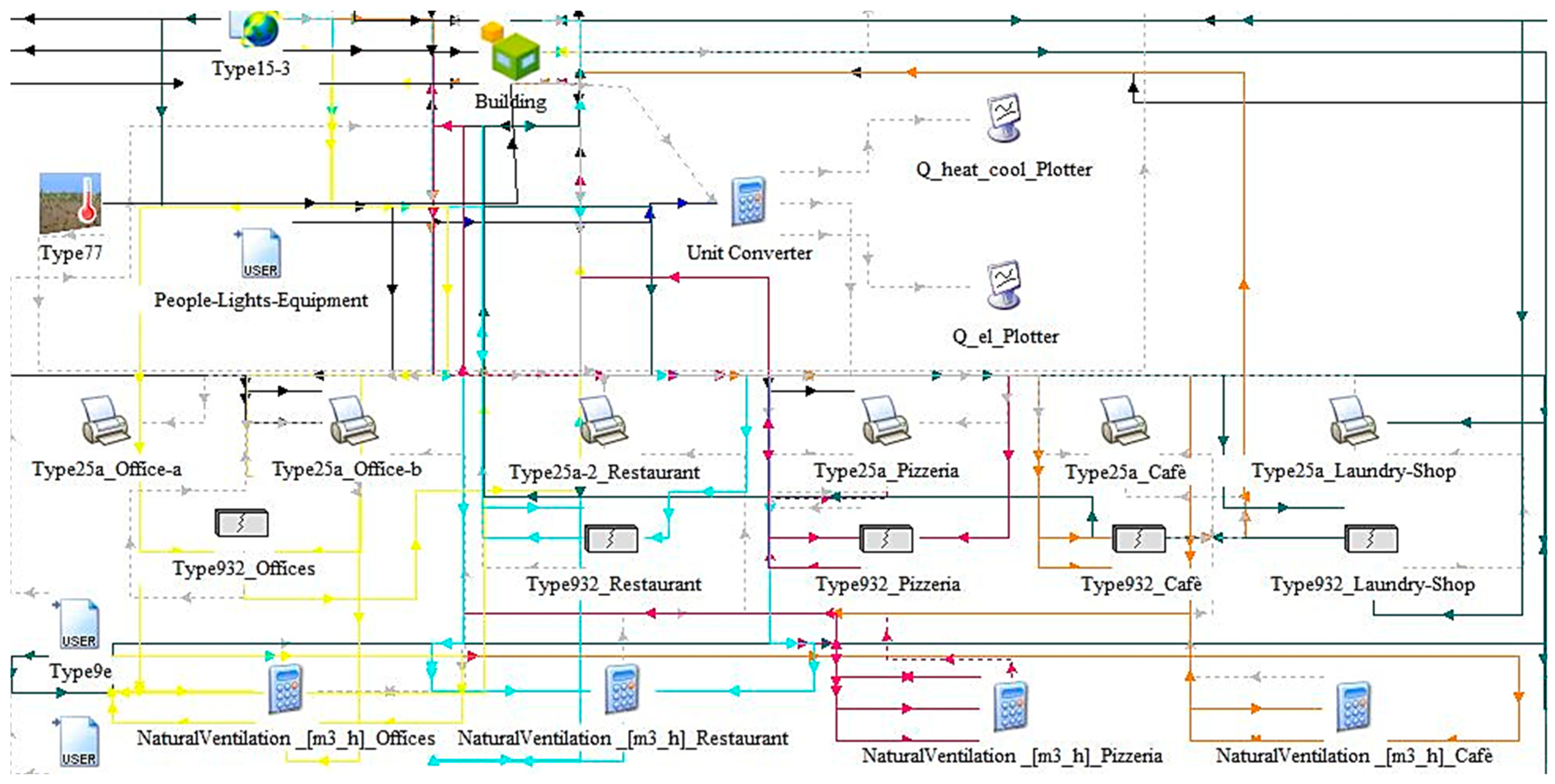
2.2. Modeling of the District and Redesign Scenarios

Consistently, with the data acquired during the site investigation, the district has been modeled in TRNSYS 18 environment and the 3D model made in SketchUp is shown in Figure 2. The 3D model contains a total of 57 thermal zones, one for each building space, and the shading elements against solar radiation have been introduced as shading generating elements. Part of the TRNSYS model in the Simulation Studio graphical environment is shown in Figure 3.

Multizone building modeling with Type 56 and TRNBUILD is used in order to model the energy and thermophysical model of buildings. The building description is transferred to the model by the building description file (*.b18,*.b17, *.bui). The main inputs of Type 56 are the climatic variables and the use and occupation profiles of the thermal zones. Occupancy differences on a hourly–daily (differences between holidays and workdays) and monthly (due to the variable activity of the city) basis were modeled in TRNSYS Simulation Studio, through specific occupation and use profiles. Climatic conditions are modeled using an EPW file (EnergyPlus Weather File) containing the historical climatic data, used as input by Type 15. Type 15 reads and interpolates the climatic data, calculating additional variables (e.g., the effective sky temperature).

The climate of Licata is characterized by temperate winters and hot summers. Figure 4 and Figure 5 describe the trend of the main climatic variables—total radiation, wind velocity, relative and external temperature (dry bulb and wet bulb temperature)—for some days in the winter period and in the summer period, for example.

The modeling of natural ventilation has been carried out according to the “Wind and Humidity Stack with Open Area” method [48] while the infiltration is modeled according to the “Sherman Grimsrud” method (Type 932) in TRNSYS [49]. Starting from the input variables (temperature, relative humidity and pressure of the zone) and parameters (volume, zone leakage area, stack coefficients and wind coefficients), the component determines the infiltration air changes and other significant terms.

To realistically represent the district in the existing configuration and obtain a consistent model, the periods of activation of the heat pumps were modeled on the basis of the real habits of the occupants through interviews and data collection carried out during the inspection phase. On average, the summer season is from May to early October, while the winter season is from December to March, although also in other periods of the year there may be a limited demand for air conditioning.

Overall, the method adopted for the energy redesign of the building complex follows several steps:

• Building energy modeling of the district and non-steady state simulation;
• Calibration of the model on the basis of monthly measured data of the electricity consumption of the building units;
• Energy efficiency solutions modeling and simulation of the calibrated model by insulating the building envelope, according to the transmittance limit values (U_lim) imposed by current Italian legislation [50] for net zero energy buildings;
• Integration of renewable energy sources through the sizing and modeling, in the TRNSYS environment, of a photovoltaic (PV) system on the roof of the buildings;
• Analysis of the results in terms of energy efficiency and interaction with the electricity grid, environmental impact of the district’s operation phase, energy flexibility of the PED scenario (called “base PED”/“PED”) according to the key performance indicators (KPIs) described in Table 2. Furthermore, the impact on thermal comfort of buildings retrofitting is evaluated on the basis of the European standard EN 16798-1 [51]. Even if the objective and scope of the study does not consist in optimizing thermal comfort, a thermal comfort analysis is carried out with the aim to assess the improvement in the thermal comfort conditions of the occupants as a co-impact of the redesign scenarios. The comfort analysis is performed by monitoring the PMV variable, based on the TRNSYS output values, and calculating the percentage of time in which the thermal comfort conditions fall within the categories I, II, III and IV defined in the standard;
• The PED energy balance is calculated, according to Equation (1), as the difference between the sum of the energy generated by the local RES systems in each time step ($\int P_{el,g}\left(t\right)dt$) and the total energy demand of the district ($\int P_{el,c}\left(t\right)dt$) over a period of one year;

  $$PED balance={\int }_{t=0}^{T=8760 h}{[P}_{el,g}\left(t\right)-P_{el,c}\left(t\right)]dt$$

  (1)
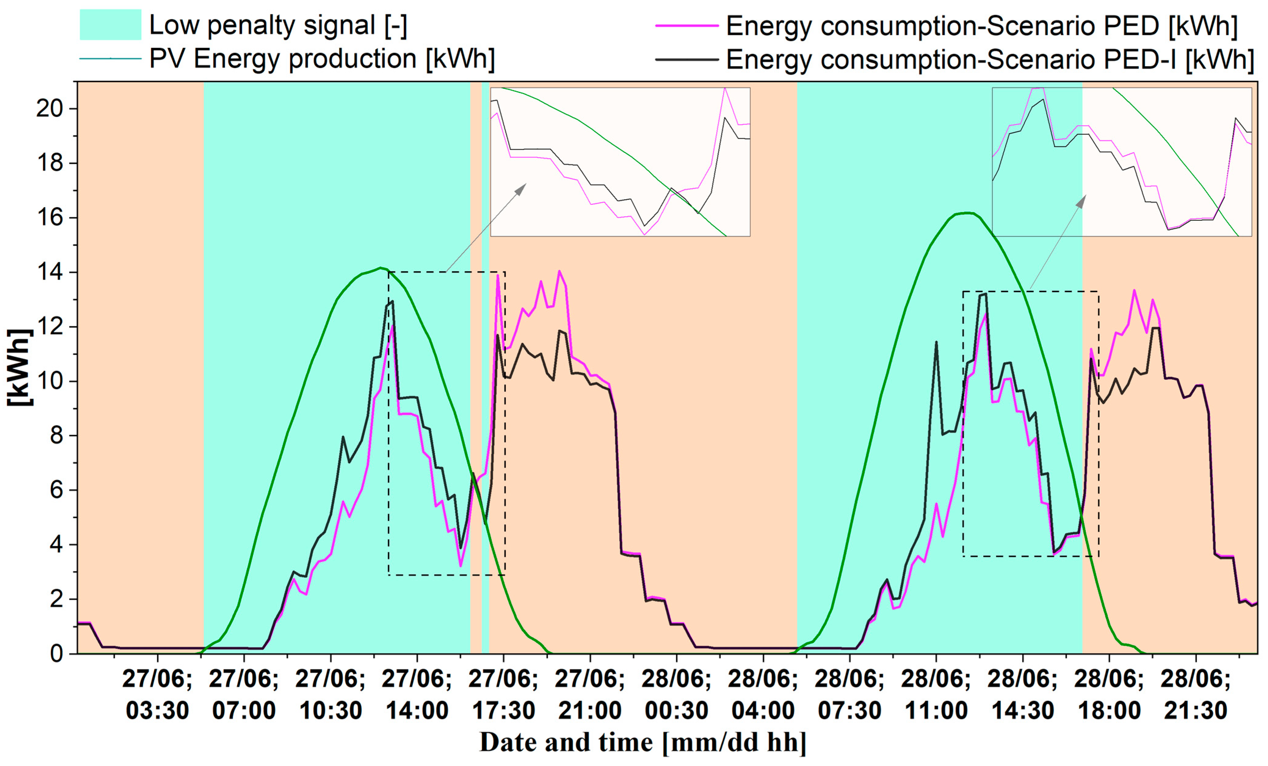
• Development and modeling of energy flexibility scenarios (PED I and PED II) based on the flexible control of the air conditioning system using rule-based control (RBC) algorithms, predicting energy consumption and production through historical climatic data.

The objective of this part is to improve the simultaneity between generation and load and the operational environmental impact of the building cluster by activating the thermal mass of the building envelope through flexible control of the air conditioning set point (T_set).

More precisely, the tested control strategies are based on the following:

(a)

Upward modulation of the space heating T_set,h during the low penalty (lp) periods and downward modulation during high penalty (hp) periods;

(b)

Upward modulation of the space cooling T_set,c during the hp periods and downward modulation during the lp periods.

The magnitude of the temperature upward and downward deviation (ΔT) is fixed at 1 °C (scenario I) and 2 °C (scenario II).

In general, the objective of a flexibility strategy is the load-shifting (e.g., derived from shifting air conditioning needs) from periods with a high penalty (hp), towards periods of low penalty (lp), properly defined according to the environmental, economic or energy perspective adopted [11,35,37,43,52,53].

In this study, high penalty periods are defined as those periods of time in which there is a deficit in energy production of the on-site photovoltaic system compared to the electricity demand of the district. On the contrary, the periods of time with a surplus of local energy production constitute the periods of low penalty.

For the calculation of energy flexibility based on emissions, low penalty periods are time steps during which electricity is produced with lower carbon footprint, considering the availability of the local solar energy production (the lp periods previously described) and the import of electricity from the grid during low emission hours.

In order to determine the low emission hours, i.e., low penalty periods, of the electricity grid the historical hourly data disclosed by Terna, the Italian electricity market operator, [54] are used. These data describe for each hour of the year the composition of the regional electricity mix (electricity mix of the electricity zone of Sicily, the region in which the city of Licata is located), in terms of the type of energy sources that constitute it for each hour, and they also provide information on the total amount of electricity produced (MWh) from each energy source, sold and fed into the electricity grid for each hour.

Figure 6 describes for two example days (days 1 and 2 of January) the composition of the regional electricity mix and the distribution for each energy source of the total amount of electricity fed into the grid for each hour of the day.

From the analysis of the data, it emerges that 100% coverage from RES never occurs during the year, while the maximum degree of energy penetration from RES is equal to 89% and occurs only for one hour a year. For the evaluation of the energy flexibility based on emissions, the hours per year for which the electricity imported from the grid is produced for at least 50% (of the total electricity fed into the grid at that hour) from renewable sources are assumed as low penalty hours. In other words, lp periods occur in the hours of the year in which the rate of penetration of energy from RES, in the regional electricity mix, is greater than 50%.

Figure 7 shows the duration curve of the penetration rate of energy from renewable sources in the regional electricity mix.

A generic point “i” on the duration curve is characterized by an ordinate value, along the y axis, equal to the generic RES penetration percentage y_i, variable in the range [0–100], and by an abscissa value equal to the value of the duration time x_i, along the x axis. The generic abscissa x_i of a point represents the number of hours per year for which the RES penetration rate remains higher than the value indicated by the corresponding ordinate y_i. As can be seen in the Figure, the RES penetration rate of the electricity mix is greater than 50% for about 30% of the hours a year, i.e., for the number of hours indicated by the abscissa of point A equal to 2596 h.

The single penalty signal is obtained from the combination of the grid penalty signal and the penalty signal relating to surplus or deficit of renewable energy produced on site from the PV system of the district. The two signals converge into a single signal which has a low penalty period as long as one of the two signals indicates a low penalty.

For the evaluation of the environmental impact of the district’s use phase, as in [11], the CO_2,eq emissions associated with the import of electricity are calculated. To do this, the emission conversion factors, c_el, for each type of energy source, expressed in [CO_2,eq/kWh] and defined in [55,56], are used.

The carbon footprint of the electricity imported from the grid is obtained from the knowledge of the qualitative and quantitative hourly composition of the regional electrical mix and from the use of the emission conversion factors. In mathematical terms and for each hour of the year, the amount of electricity in the electricity grid for the Sicily electricity zone, E(t’), is determined by the sum of the electricity produced and fed into the grid from each of the energy sources making up the electricity mix for that specific hour.

$$\begin{array}{cc}\mathrm{E}({\mathrm{t}}^{\prime })=& {\int }_0^{t^{\prime }=1 h}{(P}_{el,biomass}(t)+P_{el,fossil gas}(t)+P_{el,fossil oil}(t)+P_{el,hydro pumped storage}(t)+\\ & P_{el,hydro run-of-river}(t)+P_{el,solar}(t)+P_{el,wind onshore}(t)+P_{el,other}(t))dt\end{array}$$

(2)

Consequently and according to Equation (3), the CO_2,eq intensity of the electricity imported from the grid, ${\mathrm{I}}_{{CO}_2,eq}({\mathrm{t}}^{\prime })$, is calculated for each hour of the year using the specific conversion factors previously described.

$$\begin{array}{cc}{\mathrm{I}}_{{CO}_2,eq}({\mathrm{t}}^{\prime })=& {\int }_0^{t^{\prime }=1 h}{[(P}_{el,biomass}(t)·c_{el,biomass}(t))+{(P}_{el,fossil gas}(t)·c_{el,fossil gas}(t))\\ & +{(P}_{el,fossil oil}(t)·c_{el,fossil oil}(t))+{(P}_{el,hydro pumped storage}(t)·c_{el,hydro pumped storage}(t))\\ & +{(P}_{el,hydro run-of-river}(t)·c_{el,hydro run-of-river}(t))+{(P}_{el,solar}(t)·c_{el,solar}(t))\\ & +{(P}_{el,wind onshore}(t)·c_{el,wind onshore}(t))+{[(P}_{el,other}(t)·c_{el,other}(t))]dt\end{array}$$

(3)

Figure 8 further describes, for the 1st of January, the emission profile of the electrical mix associated to the electricity grid. The emission profile, expressed in ton CO_2,eq/MWh, represents for each time step the quantity of CO_2,eq emissions produced per MWh of electricity produced in that hour from the electricity mix and present in the electricity grid (Equation (4)).

$${(CO}_{2,eq}emissions)Emission Profile(t)=\frac{{\mathrm{I}}_{{CO}_2,eq}(\mathrm{t})}{E(t)}$$

(4)

For the evaluation of the economic impact of the energy flexibility strategies, as in [11], the operating costs associated with the import of electricity from the electricity grid are calculated. For the economic calculation, the historical hourly data of the electricity price disclosed by the Italian electricity market operator [54], for the year 2022, are used.

The operating energy costs are calculated according to Equation (5) as the product of the amount of energy imported during each hour of the year, $(\int P_{el,i}\left(t\right)dt)$ in [kWh], by the specific electricity cost in that hour ($c_{el,i}\left(t\right)$) in [€/kWh], integrated over the period of one year.

$$Operating energy costs={\int }_{t=0}^{T=8760 h}{[P}_{el,i}\left(t\right)\cdot c_{el,i}\left(t\right)]dt$$

(5)

To quantify the change from periods hp to periods lp, the flexibility factor FF is used. FF varies between −1 (consumption occurs only in hp periods) and +1 (consumption occurs in lp periods). FF (emissions) is used when low emissions periods are considered as lp periods and is linked to the objective of reducing the building’s operational emissions. On the other hand, FF (res) refers to the objective of improving the self-consumption of energy from local renewable sources in prosumer buildings and the periods lp constitute the time steps in which the production exceeds the load. To evaluate the interaction with the electricity grid, the self-consumption factor (${\mathsf{\gamma }}_s$) and the solar factor (${\mathsf{\gamma }}_L$) are used, whose formulation, except for energy and storage losses, is shown in Table 2.

The ${\mathsf{\gamma }}_L$ reports on the degree of energy coverage with solar energy generated on site, while ${\mathsf{\gamma }}_s$ on the amount of local energy production self-consumed simultaneously by the building.

Table 2. KPIs used for energy and flexibility analysis.

KPI	Symbol	Equation	Reference
Supply cover factor/Self-consumption factor	${\mathsf{\gamma }}_S$	${\mathsf{\gamma }}_s=\frac{{\int }_0^T\min \left(g\left(t\right),l\left(t\right)\right)dt}{{\int }_0^T\mathrm{g}(\mathrm{t})dt}$	[57]
Load cover factor/Solar factor	${\mathsf{\gamma }}_L$	${\mathsf{\gamma }}_L=\frac{{\int }_0^T\min \left(g\left(t\right),l\left(t\right)\right)dt}{{\int }_0^T\mathrm{l}(\mathrm{t})dt}$	[57]
Flexibility Factor	FF	$FF=\frac{{\int }_{lp}{P}_{el}dt-{\int }_{hp}{P}_{el}dt}{{\int }_{lp}{P}_{el}dt+{\int }_{hp}{P}_{el}dt}$	FF (emissions): [37], FF (res): [11]

Table 2. KPIs used for energy and flexibility analysis.

KPI	Symbol	Equation	Reference
Supply cover factor/Self-consumption factor	${\mathsf{\gamma }}_S$	${\mathsf{\gamma }}_s=\frac{{\int }_0^T\min \left(g\left(t\right),l\left(t\right)\right)dt}{{\int }_0^T\mathrm{g}(\mathrm{t})dt}$	[57]
Load cover factor/Solar factor	${\mathsf{\gamma }}_L$	${\mathsf{\gamma }}_L=\frac{{\int }_0^T\min \left(g\left(t\right),l\left(t\right)\right)dt}{{\int }_0^T\mathrm{l}(\mathrm{t})dt}$	[57]
Flexibility Factor	FF	$FF=\frac{{\int }_{lp}{P}_{el}dt-{\int }_{hp}{P}_{el}dt}{{\int }_{lp}{P}_{el}dt+{\int }_{hp}{P}_{el}dt}$	FF (emissions): [37], FF (res): [11]

3. Results and Discussion

This section shows the results of the scenario analysis which can be summarized in the following:

• The calibration of the model on the basis of real measured data;
• The analysis of the thermo-physical behavior and energy consumption of the base case (existing configuration of the district) in a dynamic regime and with a 15 min time step;
• The analysis of the results of the base PED scenario (PED configuration without the use of specific algorithms for activating the energy flexibility of the district) in terms of energy–environment and interaction with the electricity grid;
• The description and discussion of the results of the flexibility scenarios, PED I and PED II, through analysis of the grid interaction, monitored KPIs, balancing of energy flows within the district and study of the dynamic behavior in the 15 min time step;
• Comparison of the scenarios examined and discussion of the energy–environmental and economic benefits and impacts due to flexible control.

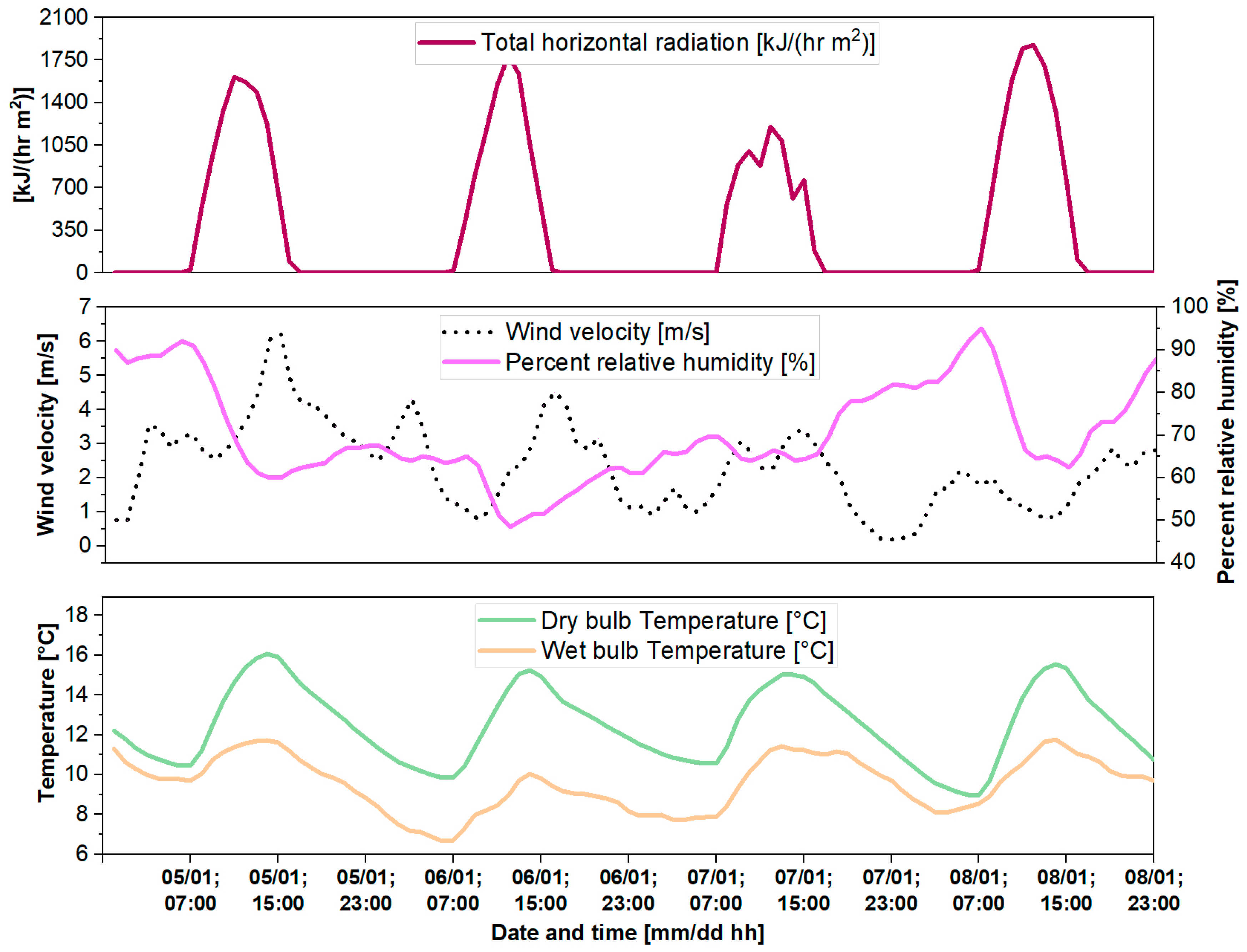
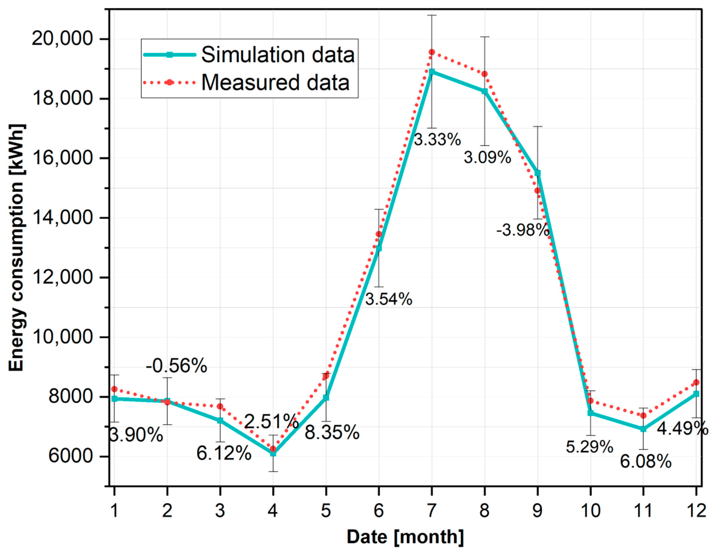
3.1. Calibration of the Model and Dynamic Analysis

The district has been simulated in its current state, obtaining monthly deviations for each building in the range [+10%, −10%] compared to the measured values of electricity consumption.

Figure 9 shows the calibration results for the entire district on a monthly basis. The gray error bars represent the range [+10%, −10%] for each monthly value of the measured energy consumption, while the two trends represent the profile of the measured energy consumption data and the profile of the energy demand simulation results of the model.

The calibrated model presents an annual electricity consumption of 125.20 MWh (0.146 MWh/m²).

The distribution of the annual electricity consumption of the district by commercial building and according to energy uses is shown Figure 10.

All the energy services used have been taken into account as follows: heating, cooling, electrical appliances (for offices, kitchens, etc.), interior lighting and lighting in the exterior area of the cafeteria, restaurant and pizzeria. The district presents a variable electricity demand profile throughout the year with higher values in the summer months. This is due on the one hand to the greater amount of energy consumption for cooling than for heating due to the climate of the place and the high internal loads in office or restaurant buildings. On the other hand, as mentioned in Section 2, part of the commercial buildings is more operational in the summer period, which is the most touristy of the year in the study area.

As for the environmental impact of the district’s use phase, the operational CO_2eq emissions are equal to 33.37 tons CO_2eq per year. FF (emissions) is equal to −0.47, which indicates that the energy demand occurs mostly during the hp periods.

Figure 11 and Figure 12 show, for a few typical days used as examples and for one of the rooms of the building cluster (one of the offices of the office building, called “Office 1”, the dynamics with 15 min time steps during the winter and summer conditions. Specifically, the Figures show, on the one hand, the dynamic trends of electricity consumption for space air-conditioning, electrical equipment and for space lighting; the main heat fluxes involved in the heat balance, on the other hand, such as heat loads due to infiltration, solar radiation, heat requirements for space air-conditioning; and finally, the trend of the PMV comfort variable and that of the air temperature and the mean surface temperature. As Figure 11 shows, as the external temperature decreases, the energy requirement for cooling during office working hours decreases (Day 3 compared to Day 1) compatibly with the internal load transmitted by the occupants (which derives from a variable degree of occupation over time), and unless the solar gain increases due to a higher value of global and total solar radiation, as for Day 2. As a result of the dynamic analysis of all thermal zones, the greatest electricity consumption for cooling occurs in zones with the highest internal loads such as for the “Office 1”, while the needs are lower in the case of the lounge area of the restaurant building. This is due both to the low value of internal thermal loads deriving from the equipment and to the presence of an internal curtain and a large external fixed structure which is located in front of the window openings. On the other hand, the internal microclimate of some areas such as the kitchen of the restaurant building and the pizzeria and the area of the pizza oven, is strongly conditioned by the high value of internal loads and little by external climatic forces.

Similar considerations can be formulated for the other zones. As Figure 12 suggests, the lack of thermal insulation causes high heat losses through the building envelope during the hours of operation of the space heating system and causes a sharp decrease in the internal air temperature when the system is switched off at the end of the working day. This downward trend determines a peak demand for heating during the first hour of the following day. Furthermore, as shown in the image, the thermal comfort conditions for the occupants could be improved due to PMV values < −0.7, indicating a prevalence of air conditioning hours in the IV comfort category [51].

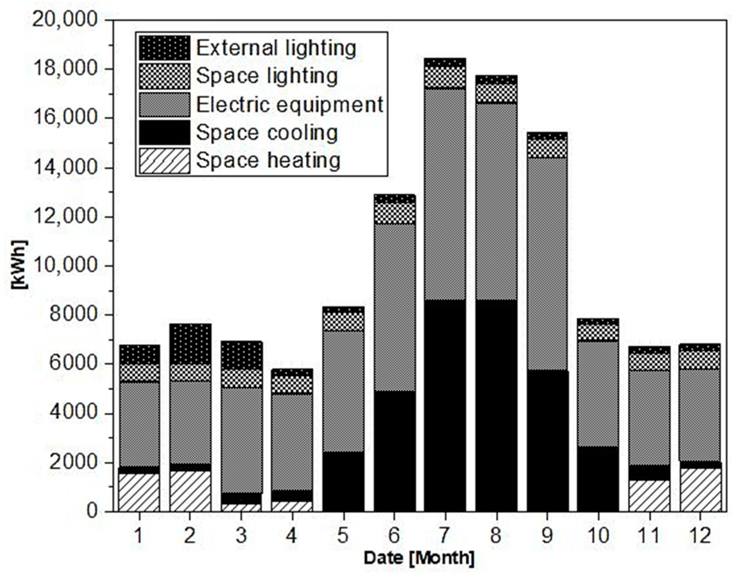
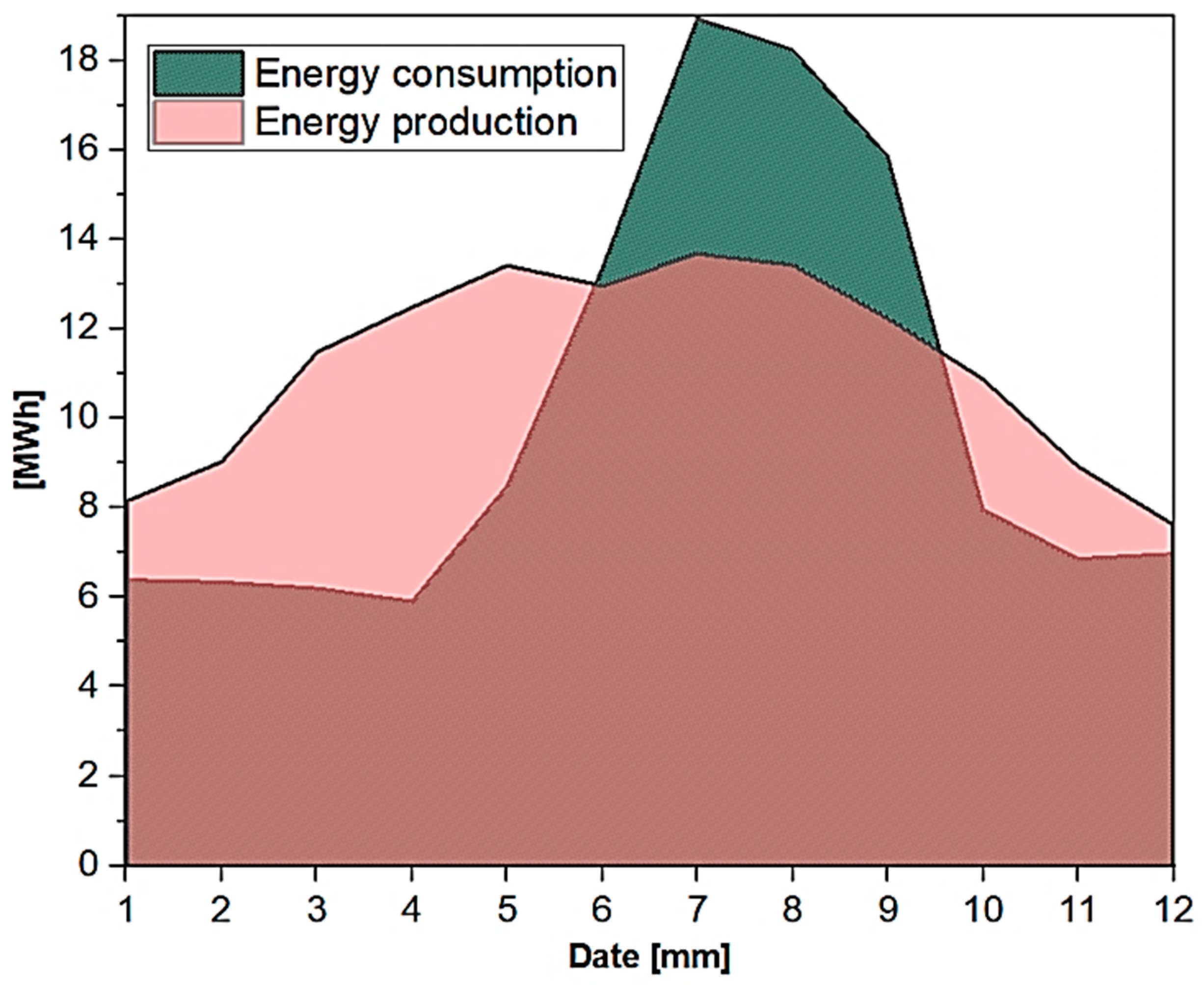
3.2. Redesign in a PED Perspective

This section summarizes the main results of the redevelopment of the district through the energy efficiency of the building envelope and the on-site integration of solar energy plants for electricity generation. Thermal insulation through the use of additional thicknesses of glass wool (6, 8, 14, cm per building component) determines compliance with the transmittance limit values, as indicated in

Table 3. Transmittance values before energy retrofitting (U*), limit (U_lim) and after retrofitting (U**).

Building Component	U*	Ulim	U**
Vertical Exterior Walls	0.77	0.38	0.358
Ground Floor	1.53	0.4	0.377
Exterior Roof	2.24	0.27	0.25
Windows	1.27	2.6	1.27

.

As regards the visualization of the dynamic behavior of the district after the insulation of the building envelope, Figure 13 and Figure 14 are shown as an example.

From the comparison of the trends ante-retrofit and post-retrofit, it can be seen that the following is the case:

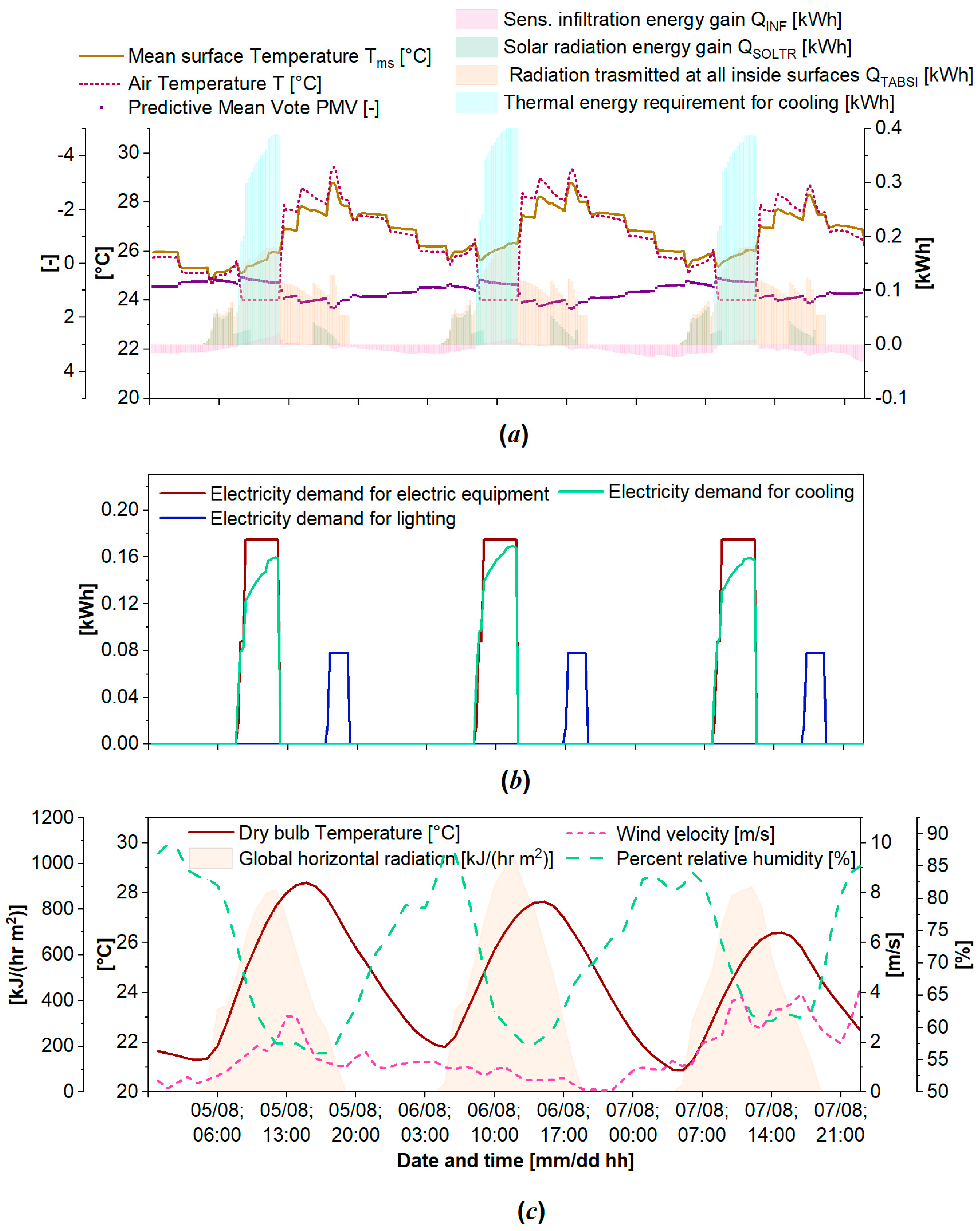
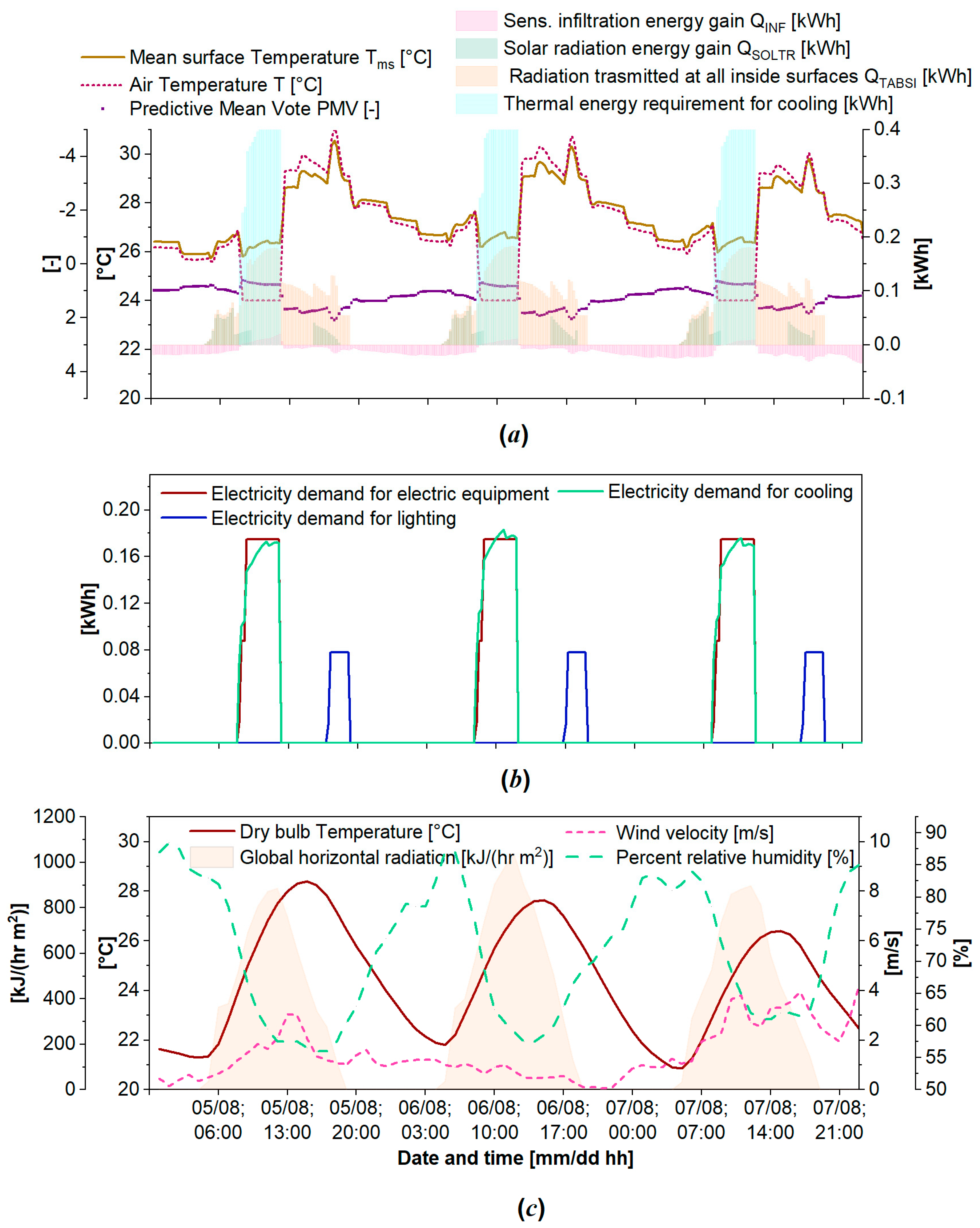
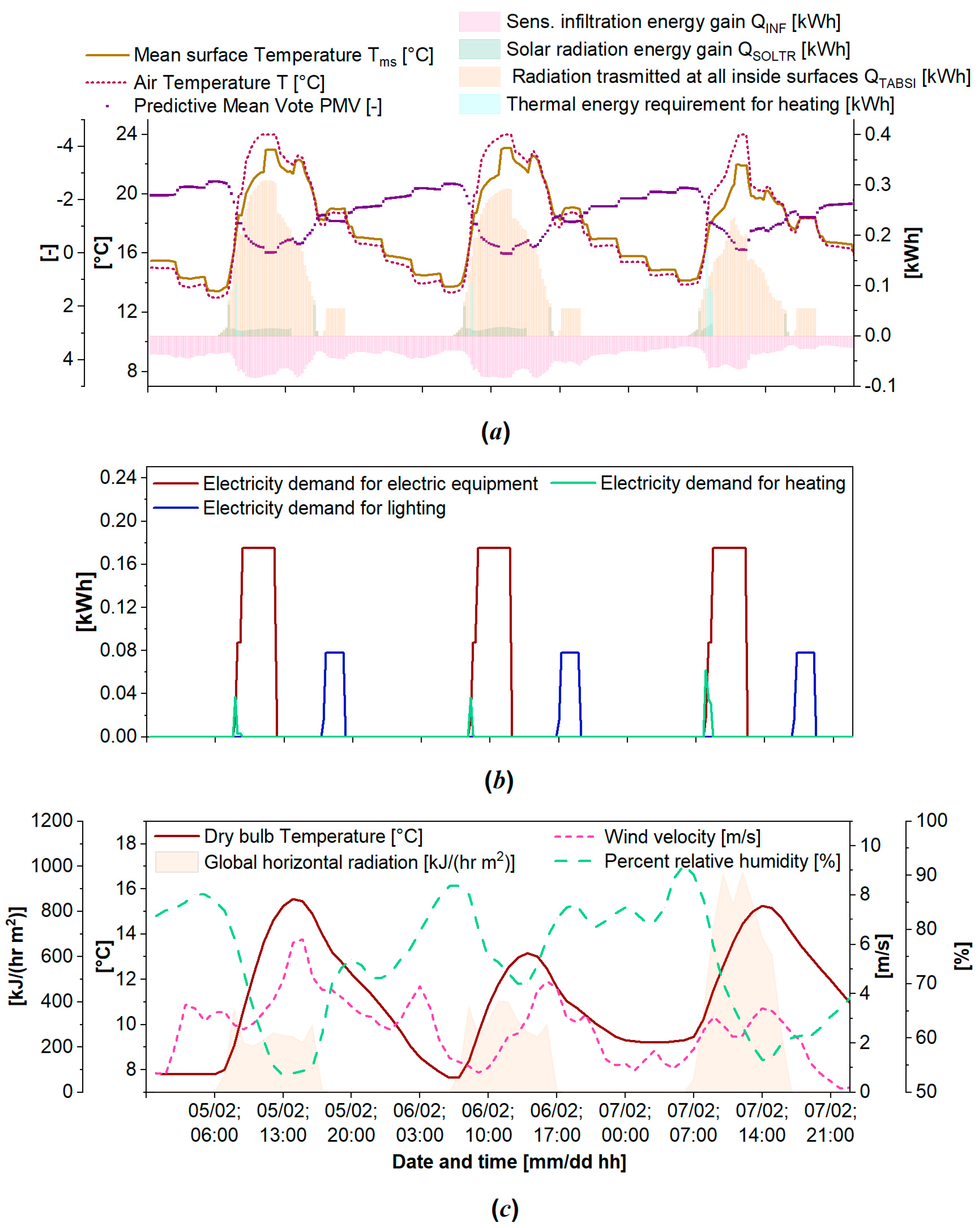
• As visible also from the PMV profile, the thermal comfort conditions have improved during the occupation time; this tendency is confirmed by the annual values reported in

  Table 4. Percentage variation, in the PED configuration, in the number of hours corresponding to the comfort categories (Cat. I, II, III, IV) compared to the existing configuration of the district (base case) for some zones used as examples.

  Comfort Cat.	Office 1	Office 4	Restaurant Hall	Cafè-Pub Hall
  Cat. I	+4%	+5.15%	+1.8%	+4%
  Cat. II	+3.29%	+4%	+5.39%	+5.46%
  Cat. III	+2.21%	+4.93%	+4.61%	+5.92%
  Cat. IV	−9.53%	−14%	−12%	−15.27%

  The minus sign (−) indicates a decrease compared to the existing case; conversely, the plus sign indicates (+) an increase.

  . In particular, as shown in Figure 11, the PMV value is close to zero in some hours of the day (Comfort Category I), for example, between 10:00 and 12:00. In the same hours in the existing configuration of the district to which Figure 9 refers, the PMV trend instead reached values close to −2, indicating a low level of thermal comfort (Comfort Category IV).
• The energy demand for space heating is about halved. As can be seen in Figure 11, the insulation of the building envelope determines a decrease in the internal air temperature of the thermal zone used as an example, which is more delayed over time and a reduction in the heating load peaks compared to the reference case.
• Regarding the cooling season, for the days displayed in the graph, the energy consumption for cooling has slightly increased, while the air temperature profile is on average higher in the hours the air-conditioning system is switched off due to the higher internal loads, caused by the lower heat transmission through the building envelope.

Figure 15 shows the distribution of the annual electricity consumption of the district by energy uses. Overall, the simulated model post-retrofit results in an annual electricity consumption of 121.45 MWh. Total energy consumption has not decreased significantly compared to the base case due to the increase in electricity demand for cooling from 25.19% to 28% of the total. On the contrary, the contribution of heating to the total demand for electricity decreases from 11.25% to 5.90%.

In the PED scenario, a photovoltaic (PV) plant of the size 83.7 kW_p (279 panels, each with an area equal to 1.63 m² and a nominal power of 300 W_p installed on the roof of the examined buildings) is also included in the energy layout.

As for the simulation results, the total electricity production is equal to 134.65 MWh/y. Figure 16 shows the monthly load and generation trend for the period of one year.

The PED model has a positive annual energy balance of 12.90 MWh and an annual self-consumption of energy equal to 59.44 MWh. The use phase of the cluster of buildings implies a value of operational emissions equal to 19.52 tons CO_2eq/y, resulting in an annual reduction of emissions of 41.50% compared to the base case.

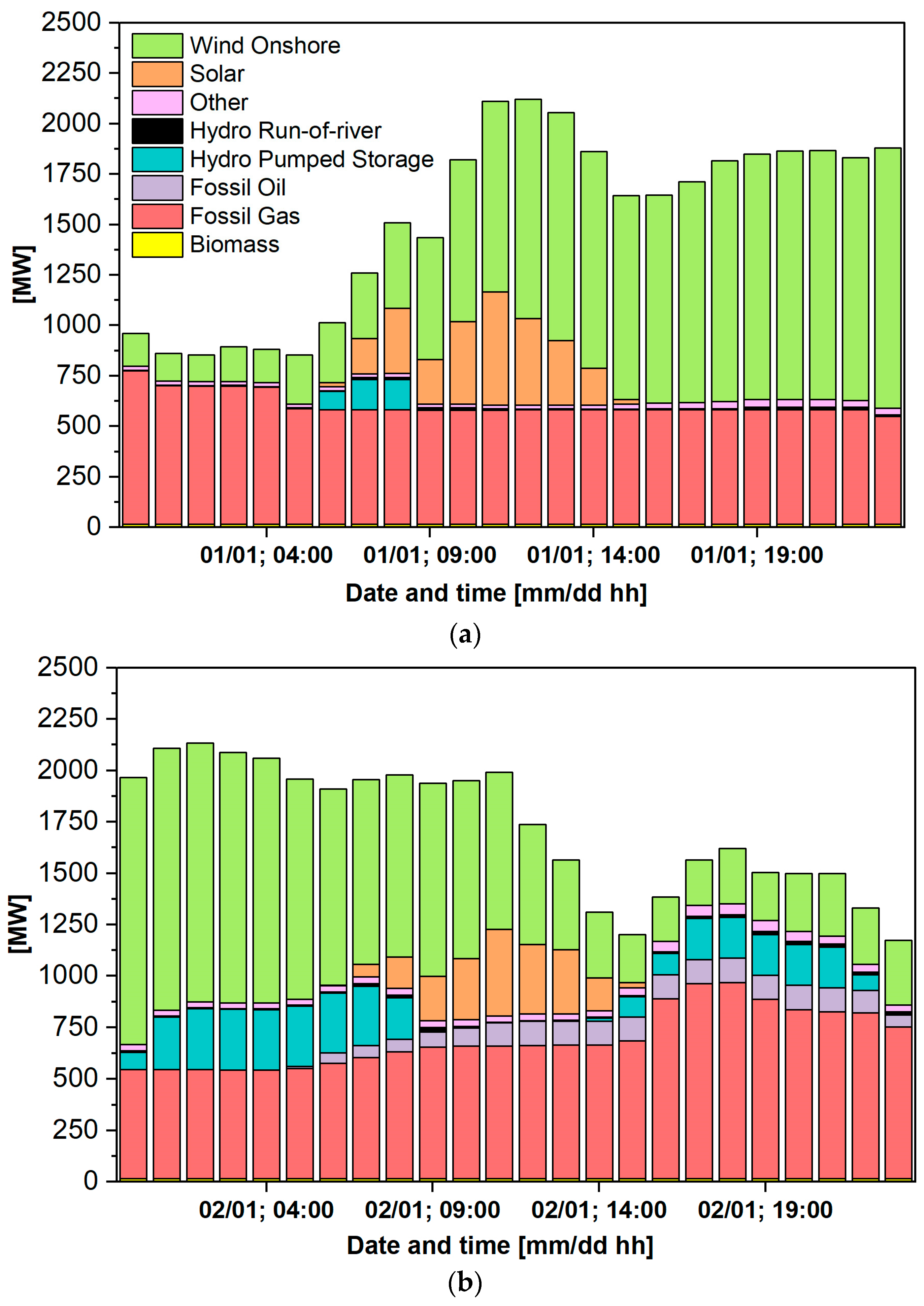
3.3. Comparison of PED Scenarios and Contribution of Energy Flexibility

This section summarizes the main results of the RBC-type energy flexibility strategies and presents a comparison of results between the different scenarios developed.

Figure 17 shows the dynamic profiles for two winter days used as an example of the local PV electricity production, the electricity demand for space heating both in the PED scenario and in the PED I scenario, and the penalty signal (green areas indicate low penalty periods, while orange areas represent high penalty periods) based on the definition of lp periods as the time step of self-produced energy surplus and vice versa as hp periods—those of deficit of local generation with respect to the energy demand. In addition, Figure 18 shows the dynamic profiles for two summer days used as an example of the local PV electricity production, the electricity demand for space cooling both in the PED scenario and in the PED I scenario, and the penalty signal. As shown in the Figures, the effect of the flexible control I determines a certain degree of load shifting from the hp periods towards those of low penalty. Considering the flexible space heating control (Figure 17), the energy consumption profile in the PED I case is above that of the base PED scenario during the lp periods due to the excess pre-heating of the buildings. Conversely, in the subsequent high penalty time steps, the electricity demand profile in the PED I case is below that of the base PED case, i.e., in the PED I scenario, a decrease in the need for space heating is observed as a rebound effect. For example, during the low penalty 8:00–13:00 on 27 February represented in Figure 17, the electrical power required in the PED I flexibility scenario is greater than that which occurs in the PED base case of about 30–40% in each time phase, due to the upwards modulation of the space-heating set point. As is visible, this causes as a rebound effect a decrease in the space heating demand in the high penalty hours (e.g., between 13:00 and 18:00) and a reduction in peak loads. A close-up of the areas of the graph where load shifting also occurs, but the graphics limit their display, is provided in the Figures. In quantitative terms and taking the first day (27 February) as an example, the daily energy consumption increases very slightly from the value of 92.11 kWh/day to 92.85 kWh/day, while the share of global consumption that occurs during lp periods increases from 38.10 kWh to 46.64 kWh. Consequently, the energy shifted from the hp periods to the lp periods is equal to 8.54 kWh. The peak load for space heating is reduced from 20.68 kW to 16.29 kW. Instead, in the case of the control algorithm which operates according to rule II (PED II scenario) and for the same day of the year, the shifted energy is greater and equal to 16 kWh and the peak load value is equal to 17.35 kW.

Considering the comparison of dynamic profiles for the two summer days (27–28 June) taken as an example, for the PED and PED-I scenario (Figure 18), it can be seen that during the lp periods the profile of the energy consumption for space cooling in the flexibility scenario exceeds that of the PED base case, due to the excess pre-cooling by exploiting the renewable energy produced on site. As a consequence, in the following hours of high penalty, e.g., between 17:00 and 21:30, there is a significant reduction in the cooling demand, which translates into a decrease in the use of energy with a higher CO_2eq intensity, through the import of electricity from the grid, and in the dependence on the electricity grid, which translates into economic and environmental benefits. Furthermore, as visible in the Figure, the flexible control does not generate an increase in the peak loads, but reduces them, contributing to lower average peak load values.

Globally,

Table 5. Comparison of the KPIs in the base scenario, PED and in the two PED scenarios (I and II) of flexibility.

Scenario	${\mathsf{\gamma }}_{\mathbf{s}}$	${\mathsf{\gamma }}_{\mathbf{L}}$	FF (Emissions)	FF (Res)
Base	-	-	−0.73	-
PED	0.44	0.49	0.06	−0.02
PED I	0.48	0.52	0.13	0.05
PED II	0.51	0.55	0.18	0.11

provides information on the annual variation of the KPIs examined as the scenario considered varies. As can be seen from the FF values, the energy flexibility improves in scenarios I and II in terms of load shifting. This is also confirmed by the trend of annual energy self-consumption that varies from 59.44 MWh in the PED scenario to 65 and 69 MWh in cases I and II, respectively, while annual imports of electricity are reduced from 62 to 58 and 55.26 MWh, and exports also reduced from 75 to 69.68 and 65.49 MWh. The trend is also confirmed in the values of ${\mathsf{\gamma }}_S$ e ${\mathsf{\gamma }}_L$, reported in the Table, and from the variation in the mapping during the year to the variation of the scenario considered, shown in Figure 19.

In fact, as can be seen in Figure 16, going from the basic PED scenario to the PED II scenario, some areas change their color from yellow/green to red, indicating an increase in the self-consumption factor (${\mathsf{\gamma }}_s$) which represents an increase in the amount of local energy production self consumed simultaneously by the district. This occurs, for example, between days 300 and 360, corresponding to the months of November and December between 8:00 and 16:00, or for example in the month of October and all the others clearly visible between 8:00–12:00, and also in the rest of the hours of availability of local energy generation.

Regarding the environmental impact of the strategies, considering FF (emissions), the annual rate of energy consumption that occurs during the low penalty periods increases by 7% in scenario I, and by 12% in scenario II, compared to the PED scenario.

The impact of the use phase of the district is equal to 18.41 and to 17.39 tons CO_2eq/y in the PED I and PED II scenario, respectively. From an economic point of view, in the redesign scenarios that include the activation of the energy flexibility of the thermal building mass, the operating costs related to energy are reduced by 50% compared to the existing base case and by approximately 12% compared to the PED base case.

As in previous applications, e.g., [11,31,43], the implementation of algorithms for the flexible management of the air conditioning system achieves good performance of the order of 10–20% reduction in emissions and operating costs, even in the case where the penalty signal is based on the availability of renewable energy produced within the confines of the PED in the Mediterranean climate, as in [58], with results in line also from the point of view of the energy–environmental impact of building retrofitting.

Figure 20 shows the evolution of the PED balance and the reduction in operational CO_2eq emissions per year, compared to the existing base case in the scenarios analyzed. In this case, the application of flexibility strategies does not significantly affect the PED balance, understood as a mere numerical subtraction value between energy generation and consumption, but it does contribute substantially to improving the energy–environmental efficiency of the district with an acceptable impact on peak loads.

4. Conclusions

This paper presents the energy retrofitting from a PED perspective of a building district located in the Mediterranean area in order to evaluate its energy–environmental behavior in a dynamic regime, on the one hand, and to study the energy flexibility potential of the district in relation to the implementation of some strategies in the other.

Some scenarios based on the analysis of energy rehabilitation, integration of solar energy and activation of energy flexibility are described in this paper. Results are discussed in terms of interaction with the electricity grid, operational CO_2eq emissions, some flexibility KPIs, the analysis of the energy flows and the PED energy balance.

The findings show that the district retrofitting allows to achieve the PED status, determining a reduction in the air conditioning needs of about 50% and an improvement in the thermal comfort conditions of the occupants (percentage variation in the number of hours corresponding to the Comfort Categories IV, compared to the existing configuration of the district, on average equal to −13%.)

The joint action of energy efficiency strategies (insulation of the building envelope and use of solar energy) and energy flexibility improves the environmental sustainability of the district and the balance of energy flows. In fact, when the flexible control logics of the space air conditioning system are taken into account in the PED, an additional margin of reduction in operational CO_2eq emissions and an increase in self-consumption of energy of approximately 10% is achieved, improving the contemporaneity between generation and load. Furthermore, from the point of view of the economic impact on the use phase of the district, the activation of energy flexibility contributes a further margin of about 12% of economic savings for the purchase of energy, with a positive impact on peak loads.

However, given that the thermal insulation of the building envelope has determined a significant increase in energy consumption for cooling, it should also be noted that adaptation to the transmittance limit values imposed by current legislation does not always achieve optimal performance in terms of energy efficiency, especially in regions with a Mediterranean climate and particularly in buildings with high internal loads, such as restaurants.

As for the energy flexibility analysis and as indicated by the energy flexibility KPIs, the implementation of RBC algorithms for the flexible control determines a significant load shifting from the high penalty periods towards those of low penalty. This determines the activation of the energy flexibility of the district and of the thermal mass, e.g., by means of programmed pre-heating of the rooms and the consequent storage of energy. The approach contributes to the self-sufficiency of the positive energy district and the simultaneity of energy demand and on-site renewable energy generation. As a result, the operational emissions of the district vary from the base value of 33.37 tons CO_2eq/y to 19.52 tons CO_2eq/y in the scenario based on the integration of solar energy systems and energy efficiency measures, and to 17.39 tons CO_2eq/y when the demand-side energy flexibility is also activated.

It should be noted that these findings are achieved due to the automatic flexible control which, unlike the installation of an energy storage device, does not imply additional installation costs in the design phase, nor an increase in the embodied emissions of the system. However, due to the induced temperature variations, thermal comfort could be jeopardized. Therefore, the need for a comfort analysis for each of the rooms should be prioritized in order to avoid conditions of discomfort for the occupants and, indeed, guide the algorithm in the choice of control logics that operate according to the direction of improvement of comfort.

On the other hand, since the impact of energy efficiency and energy flexibility strategies also varies depending on the use of buildings, an analysis at both the disaggregated and aggregated district level could be useful to move towards optimized solutions.

As for the PED energy balance, although the activation of energy flexibility has caused an appreciable improvement in all the grid interaction KPIs and a significant increase in FFs, the energy balance understood as a mere numerical value is not greatly affected by the effect of flexible control and is reduced to the increase in flexibility.

Therefore, the importance of a broad and deep analysis of energy flows and flexibility KPIs also arises since a partial analysis or based on the mere evaluation of the PED energy balance could lead to misleading conclusions.

Regarding the limitations of this paper, it should be noted that although the economic impact of the implementation of the flexibility strategies investigated in this research work has been evaluated (with respect to both the existing base case and the PED base case in which they are not applied), it does not provide a detailed overview of the costs due to the retrofitting of buildings and to life cycle costs, as these are outside the scope of the paper. These aspects will be dealt with in detail in future research outputs which aim to investigate the economic–social and environmental sustainability of redesign approaches from a PED perspective.

In conclusion, the research results of this work translate into a series of lessons learned that can be extrapolated to similar contexts in the Mediterranean area and stimulate considerations for future research outlooks. In particular, future perspectives should focus on the following: (a) a multi-criteria approach aimed at activating energy flexibility in PEDs, (b) an in-depth analysis of occupant comfort in order to investigate possible significant impacts, and (c) the development of a holistic design framework for PEDs that builds elements of energy flexibility and sustainability (environmental, economic and social).

References

1. United Nations Climate Change. Paris Agreement; United Nations Climate Change: Bonn, Germany, 2015. [Google Scholar]
2. European Commission. European Commission, Green Deal. 2019. Available online: https://ec.europa.eu/info/strategy/priorities-2019-2024/european-green-deal_it (accessed on 18 February 2021).
3. IPCC. Climate Change 2022—Mitigation of Climate Change—Working Group III. Cambridge University Press, 1454. 2022. Available online: https://www.ipcc.ch/report/ar6/wg3/ (accessed on 20 January 2020).
4. United Nations. The Sustainable Development Goals Report; UN: New York, NY, USA, 2020. [Google Scholar]
5. United Nations. Work of the Statistical Commission pertaining to the 2030 Agenda for Sustainable Development (A/RES/71/313). In Resolution Adopted by the General Assembly on 6 July 2017. 71/313. Work of the Statistical Commission Pertaining to the 2030 Agenda for Sustainable Development; UN: New York, NY, USA, 2017. [Google Scholar]
6. IEA.; UN. Global Status Report for Buildings and Construction: Towards a Zero-Emission, Efficient and Resilient Buildings and Construction Sector. 2019. Available online: https://webstore.iea.org/download/direct/2930?filename=2019_global_status_report_for_buildings_and_construction.pdf (accessed on 20 January 2020).
7. IEA. World Energy Outlook 2019-GlobalABC Regional Roadmap for Buildings and Construction in Asia 2020–2050 (World Energy Outlook); OECD: Paris, France, 2019. [Google Scholar] [CrossRef]
8. IEA. Perspectives for the Clean Energy Transition. 2019. Available online: https://www.iea.org/reports/the-critical-role-of-buildings (accessed on 20 January 2020).
9. Ceglia, F.; Marrasso, E.; Pallotta, G.; Roselli, C.; Sasso, M. The State of the Art of Smart Energy Communities: A Systematic Review of Strengths and Limits. Energies 2022, 15, 3462. [Google Scholar] [CrossRef]
10. Campos, I.; Marín-González, E. People in transitions: Energy citizenship, prosumerism and social movements in Europe. Energy Res. Soc. Sci. 2020, 69, 101718. [Google Scholar] [CrossRef]
11. Marotta, I.; Guarino, F.; Cellura, M.; Longo, S. Investigation of design strategies and quantification of energy flexibility in buildings: A case-study in southern Italy. J. Build. Eng. 2021, 41, 102392. [Google Scholar] [CrossRef]
12. Airò Farulla, G.; Tumminia, G.; Sergi, F.; Aloisio, D.; Cellura, M.; Antonucci, V.; Ferraro, M. A Review of Key Performance Indicators for Building Flexibility Quantification to Support the Clean Energy Transition. Energies 2021, 14, 5676. [Google Scholar] [CrossRef]
13. Sareen, S.; Albert-Seifried, V.; Aelenei, L.; Reda, F.; Etminan, G.; Andreucci, M.-B.; Kuzmic, M.; Maas, N.; Seco, O.; Civiero, P.; et al. Ten questions concerning positive energy districts. Build. Environ. 2022, 216, 109017. [Google Scholar] [CrossRef]
14. European Commission. Directive (EU) 2018/844 of the European Parliament and of the Council of 30 May 2018 Amending Directive 2010/31/EU on the Energy Performance of Buildings and Directive 2012/27/EU on Energy Efficiency; European Commission: Brussels, Belgium, 2018. [Google Scholar]
15. Gouveia, J.P.; Seixas, J.; Palma, P.; Duarte, H.; Luz, H.; Cavadini, G.B. Positive Energy District: A Model for Historic Districts to Address Energy Poverty. Front. Sustain. Cities 2021, 3, 648473. [Google Scholar] [CrossRef]
16. Leone, F.; Reda, F.; Hasan, A.; Rehman, H.U.; Nigrelli, F.C.; Nocera, F.; Costanzo, V. Lessons Learned from Positive Energy District (PED) Projects: Cataloguing and Analysing Technology Solutions in Different Geographical Areas in Europe. Energies 2023, 16, 356. [Google Scholar] [CrossRef]
17. Hedman, Å.; Rehman, H.U.; Gabaldón, A.; Bisello, A.; Albert-Seifried, V.; Zhang, X.; Guarino, F.; Grynning, S.; Eicker, U.; Neumann, H.-M.; et al. IEA EBC Annex83 positive energy districts. Buildings 2021, 11, 130. [Google Scholar] [CrossRef]
18. Lindholm, O.; Rehman, H.U.; Reda, F. Positioning Positive Energy Districts in European Cities. Buildings 2021, 11, 19. [Google Scholar] [CrossRef]
19. European Union. SET-Plan Working Group. SET-Plan Action No 3.2 Implementation Plan-Europe to Become a Global Role Model in Integrated, Innovative Solutions for the Planning, Deployment, and Replication of Positive Energy Districts. 2018. (Issue June). Available online: https://setis.ec.europa.eu/system/files/setplan_smartcities_implementationplan.pdf (accessed on 20 January 2020).
20. JPI Urban Europe. Europe Towards Positive Energy Districts. PED Booklet (Issue February). 2020. Available online: https://jpi-urbaneurope.eu/wp-content/uploads/2020/06/PED-Booklet-Update-Feb-2020_2.pdf, (accessed on 20 January 2020).
21. JPI Urban Europe. Positive Energy Districts (PED). 2021. Available online: https://jpi-urbaneurope.eu/ped/ (accessed on 21 March 2021).
22. Erba, S.; Pagliano, L. Combining Sufficiency, Efficiency and Flexibility to Achieve Positive Energy Districts Targets. Energies 2021, 14, 4697. [Google Scholar] [CrossRef]
23. Cutore, E.; Volpe, R.; Sgroi, R.; Fichera, A. Energy management and sustainability assessment of renewable energy communities: The Italian context. Energy Convers. Manag. 2023, 278, 116713. [Google Scholar] [CrossRef]
24. Tonellato, G.; Kummert, M.; Candanedo, J.A.; Beaudry, G.; Pasquier, P. Control strategy evaluation framework for ground source heat pumps using standing column wells. In Proceedings of the IGSHPA Research Track 2022, Las Vegas, NV, USA, 6–8 December 2022; pp. 246–255. [Google Scholar] [CrossRef]
25. Marotta, I.; Guarino, F.; Longo, S.; Cellura, M. Environmental Sustainability Approaches and Positive Energy Districts: A Literature Review. Sustainability 2021, 13, 13063. [Google Scholar] [CrossRef]
26. Tuerk, A.; Frieden, D.; Neumann, C.; Latanis, K.; Tsitsanis, A.; Kousouris, S.; Llorente, J.; Heimonen, I.; Reda, F.; Ala-Juusela, M.; et al. Integrating Plus Energy Buildings and Districts with the EU Energy Community Framework: Regulatory Opportunities, Barriers and Technological Solutions. Buildings 2021, 11, 468. [Google Scholar] [CrossRef]
27. Li, R.; Satchwell, A.J.; Finn, D.; Christensen, T.H.; Kummert, M.; Le Dréau, J.; Lopes, R.A.; Madsen, H.; Salom, J.; Henze, G.; et al. Ten questions concerning energy flexibility in buildings. Build. Environ. 2022, 223, 109461. [Google Scholar] [CrossRef]
28. Jensen, S.Ø.; Marszal-Pomianowska, A.; Lollini, R.; Pasut, W.; Knotzer, A.; Engelmann, P.; Stafford, A.; Reynders, G. IEA EBC Annex 67. Energy Flex. Build. 2017, 155, 25–34. [Google Scholar] [CrossRef]
29. International Energy Agency. Position Paper of the IEA Energy in Buildings and Communities Program (EBC) Annex 67. Energy Flex. Build. 2017, 1–16. [Google Scholar]
30. Li, H.; Wang, Z.; Hong, T.; Piette, M.A. Energy flexibility of residential buildings: A systematic review of characterization and quantification methods and applications. Adv. Appl. Energy 2021, 3, 100054. [Google Scholar] [CrossRef]
31. Péan, T.; Salom, J.; Ortiz, J. Environmental and Economic Impact of Demand Response Strategies for Energy Flexible Buildings. In Proceedings of the Building Simulation and Optimization BSO 2018, Cambridge, UK, 11–12 September 2018; pp. 277–283. [Google Scholar]
32. Junker, R.G.; Azar, A.G.; Lopes, R.A.; Lindberg, K.B.; Reynders, G.; Relan, R.; Madsen, H. Characterizing the energy flexibility of buildings and districts. Appl. Energy 2018, 225, 175–182. [Google Scholar] [CrossRef]
33. Tang, H.; Wang, S.; Li, H. Flexibility categorization, sources, capabilities and technologies for energy-flexible and grid-responsive buildings: State-of-the-art and future perspective. Energy 2021, 219, 119598. [Google Scholar] [CrossRef]
34. Finck, C.; Beagon, P.; Clauß, J.; Pean, T.; Vogler-Finck, P.J.C.; Zhang, K.; Kazmi, H. Review of applied and tested control possibilities for energy flexibility in buildings: A technical report from IEA EBC Annex 67. Energy Flex. Build. 2017, 1–59. [Google Scholar] [CrossRef]
35. Péan, T.Q.; Salom, J.; Ortiz, J. Potential and optimization of a price-based control strategy for improving energy flexibility in Mediterranean buildings. Energy Procedia 2017, 122, 463–468. [Google Scholar] [CrossRef]
36. Péan, T.; Torres, B.; Salom, J.; Ortiz, J. Representation of daily profiles of building energy flexibility. In Proceedings of the ESim 2018, the 10th Conference of IBPSA-Canada, Montréal, QC, Canada, 9–10 May 2018; pp. 153–162. [Google Scholar]
37. Péan, T.; Costa-Castelló, R.; Salom, J. Price and carbon-based energy flexibility of residential heating and cooling loads using model predictive control. Sustain. Cities Soc. 2019, 50, 101579. [Google Scholar] [CrossRef]
38. Taddeo, P.; Colet, A.; Carrillo, R.E.; Canals, L.C.; Schubnel, B.; Stauffer, Y.; Bellanco, I.; Garcia, C.C.; Salom, J. Management and Activation of Energy Flexibility at Building and Market Level: A Residential Case Study. Energies 2020, 13, 1188. [Google Scholar] [CrossRef]
39. Masy, G.; Georges, E.; Verhelst, C.; Lemort, V.; André, P. Smart grid energy flexible buildings through the use of heat pumps and building thermal mass as energy storage in the Belgian context. Sci. Technol. Built Environ. 2015, 21, 800–811. [Google Scholar] [CrossRef]
40. Clauß, J.; Finck, C.; Vogler-finck, P.; Beagon, P. Control strategies for building energy systems to unlock demand side flexibility—A review. In Proceedings of the 15th International Conference of the International Building Performance, San Francisco, CA, USA, 7–9 August 2017; pp. 611–620. [Google Scholar]
41. Majdalani, N.; Aelenei, D.; Lopes, R.A.; Silva, C.A.S. The potential of energy flexibility of space heating and cooling in Portugal. Util. Policy 2020, 66, 101086. [Google Scholar] [CrossRef]
42. Salpakari, J.; Lund, P. Optimal and rule-based control strategies for energy flexibility in buildings with PV. Appl. Energy 2016, 161, 425–436. [Google Scholar] [CrossRef]
43. Fitzpatrick, P.; D’ettorre, F.; De Rosa, M.; Yadack, M.; Eicker, U.; Finn, D.P. Influence of electricity prices on energy flexibility of integrated hybrid heat pump and thermal storage systems in a residential building. Energy Build. 2020, 223, 110142. [Google Scholar] [CrossRef]
44. Rehman, O.A.; Palomba, V.; Frazzica, A.; Cabeza, L.F. Enabling Technologies for Sector Coupling: A Review on the Role of Heat Pumps and Thermal Energy Storage. Energies 2021, 14, 8195. [Google Scholar] [CrossRef]
45. Tonellato, G.; Heidari, A.; Pereira, J.; Carnieletto, L.; Flourentzou, F.; De Carli, M.; Khovalyg, D. Optimal design and operation of a building energy hub: A comparison of exergy-based and energy-based optimization in Swiss and Italian case studies. Energy Convers. Manag. 2021, 242, 114316. [Google Scholar] [CrossRef]
46. Vigna, I.; Pernetti, R.; Pasut, W.; Lollini, R. New domain for promoting energy efficiency: Energy Flexible Building Cluster. Sustain. Cities Soc. 2018, 38, 526–533. [Google Scholar] [CrossRef]
47. CIES22. Libro de Actas del XVIII Congreso Ibérico y XIV Congreso Iberoamericano de Energía Solar. 2023. Available online: https://owncloud.uib.es/index.php/s/tmkYMiGqZPeR8AT?dir=undefined&openfile=16318142 (accessed on 20 April 2023).
48. DOE. Engineering Reference of EnergyPlus; DOE: Washington, DC, USA, 2017; pp. 1–1704. [Google Scholar]
49. Klein, S.A.; Beckman, W.A.; Mitchell, J.W.; Duffie, J.A.; Duffie, N.A.; Freeman, T.L.; Mitchell, J.C.; Braun, J.E.; Evans, B.L.; Kummer, J.P.; et al. TRNSYS 18 Manual, Volume 4: Mathematical Reference. Available online: https://studylib.net/doc/26018127/trnsys18-%E2%80%93-mathematical-reference (accessed on 20 January 2020).
50. Italian Government-Ministry of Economic Development. Decreto Efficienza Energetica. 2020. Available online: https://st3.idealista.it/news/archivie/2020-08/decreto_efficienza_energetica_2020.pdf (accessed on 8 June 2022).
51. European Committee for Standardization. EN 15251; Indoor Environmental Input Parameters for Design and Assessment of Energy Performance of Buildings-Addressing Indoor Air Quality, Thermal Environment, Lighting and Acoustics. European Committee for Standardization: Brussels, Belgium, 2008.
52. Mugnini, A.; Coccia, G.; Polonara, F.; Arteconi, A. Energy Flexibility as Additional Energy Source in Multi-Energy Systems with District Cooling. Energies 2021, 14, 519. [Google Scholar] [CrossRef]
53. Marotta, I.; Guarino, F.; Cellura, M.; Longo, S. Energy flexibility in Mediterranean buildings: A case-study in Sicily. E3S Web Conf. 2020, 197, 02002. [Google Scholar] [CrossRef]
54. European Union-Entsoe. 2021. Available online: https://transparency.entsoe.eu/ (accessed on 20 April 2022).
55. Ispra, R. Fattori di Emissione Atmosferica di Gas a Effetto Serra Nel Settore Elettrico Nazionale e Nei Principali Paesi Europei. 2019. Available online: https://www.isprambiente.gov.it/it/pubblicazioni/rapporti/fattori-di-emissione-atmosferica-di-gas-a-effetto-serra-nel-settore-elettrico-nazionale-e-nei-principali-paesi-europei (accessed on 20 January 2020).
56. IPCC. Climate Change 2014 Mitigation of Climate Change. In Climate Change 2014 Mitigation of Climate Change; Intergovernmental Panel on Climate Change: Geneva, Switzerland, 2014. [Google Scholar] [CrossRef]
57. Salom, J.; Marszal, A.J.; Widén, J.; Candanedo, J.; Lindberg, K.B. Analysis of load match and grid interaction indicators in net zero energy buildings with simulated and monitored data. Appl. Energy 2014, 136, 119–131. [Google Scholar] [CrossRef]
58. Andresen, I.; Healey Trulsrud, T.; Finocchiaro, L.; Nocente, A.; Tamm, M.; Ortiz, J.; Salom, J.; Magyari, A.; Oeffelen, L.H.-v.; Borsboom, W.; et al. Design and performance predictions of plus energy neighbourhoods—Case studies of demonstration projects in four different European climates. Energy Build. 2022, 274, 112447. [Google Scholar] [CrossRef]
Figure 1. Photographic description and location of the case study.
Solar 03 00016 g001
Figure 2. TRNSYS 3D model in SketchUp environment of the building cluster.
Solar 03 00016 g002
Figure 3. Part of the TRNSYS Simulation Studio model of the building cluster.
Solar 03 00016 g003
Figure 4. Trend of the main climatic variables for some winter days used as examples.
Solar 03 00016 g004
Figure 5. Trend of the main climatic variables for some summer days used as examples.
Solar 03 00016 g005
Figure 6. Composition of the regional electricity mix and the distribution for each energy source of the total amount of electricity fed into the grid for each hour of the day. Example for the 1st (a) and 2nd (b) of January.
Solar 03 00016 g006
Figure 7. Duration curve of the penetration rate of energy from renewable sources in the regional electricity mix.
Solar 03 00016 g007
Figure 8. Composition of the regional electricity mix associated to the electricity grid and CO2,eq emission profile. Example for 1 January.
Solar 03 00016 g008
Figure 9. Calibration results of the district model on a monthly and aggregated basis.
Solar 03 00016 g009
Figure 10. Distribution of the annual electricity consumption of the district by energy use (a) and per building (b).
Solar 03 00016 g010
Figure 11. Thermophysical and energy behavior of “Office 1” of the office building and 15 min time-step profiles of the main variables for some days of the summer period (5–7 August) used as examples. (a) thermal comfort variables, thermal energy requirement for air-conditioning, energy gains and losses; (b) electricity demand by energy use; (c) main climatic variables.
Solar 03 00016 g011
Figure 12. Thermophysical and energy behavior of “Office 1” of the office building and 15 min time-step profiles of the main variables for some days of the winter period (5–7 February) used as examples. (a) thermal comfort variables, thermal energy requirement for air-conditioning, energy gains and losses; (b) electricity demand by energy use; (c) main climatic variables.
Solar 03 00016 g012
Figure 13. Thermophysical and energy behavior of “Office 1” of the office building in the PED base scenario, 15 min time-step profiles of the main variables for some days from the summer period (5–7 August) used as an example. (a) thermal comfort variables, thermal energy requirement for air-conditioning, energy gains and losses; (b) electricity demand by energy use; (c) main climatic variables.
Solar 03 00016 g013
Figure 14. Thermophysical and energy behavior of “Office 1” of the office building in the PED base scenario, 15 min time-step profiles of the main variables for some days from the winter period (5–7 February) used as example- (a) thermal comfort variables, thermal energy requirement for air-conditioning, energy gains and losses; (b) electricity demand by energy use; (c) main climatic variables.
Solar 03 00016 g014
Figure 15. Distribution of the annual electricity consumption of the district by energy uses in the post-retrofit scenario.
Solar 03 00016 g015
Figure 16. Electricity consumption and generation on a monthly basis in the PED scenario.
Solar 03 00016 g016
Figure 17. Comparison of dynamic profiles for two winter days (27–28 February) for the PED and PED-I scenario.
Solar 03 00016 g017
Figure 18. Comparison of dynamic profiles for two summer days (27–28 June) for the PED and PED-I scenario.
Solar 03 00016 g018
Figure 19. Comparison of γ s map in the PED scenario (a), PED I (b) scenario and PED II case (c).
Solar 03 00016 g019aSolar 03 00016 g019b
Figure 20. Evolution of the PED balance and the reduction in operational CO2eq emissions compared to the base case.
Solar 03 00016 g020