Temporal Resolution of Input Weather Data Strongly Affects an Off-Grid PV System Layout and Reliability

Abstract

Renewable energy systems design using average year weather data is a standard approach that works well for grid-tied systems, but for stand-alone ones, it leads to dramatic mistakes. We considered the effect of meteorological data temporal resolution (5, 10, 15, 20, 30 min; 1, 2, 3, 4 h) on a stand-alone hybrid system’s layout in terms of equipment cost, power supply reliability and maximum duration of interruption for monitoring equipment in the Alps. We have shown that lifecycle costs could be strongly (order of magnitude) underestimated for off-grid systems, as well as their reliability overestimated. Lower temporal resolution data lead to the underestimation of energy storage charge–discharge cycles (considering depth of discharge too)—real batteries are to be replaced more often, which matches our practical experience as well. Even a 5 to 10 min decrease in weather data temporal resolution leads to the estimated annual expenses being halved. In general, we recommend using 30 min resolution.

1. Introduction

During the off-grid power supply design process, it is necessary to make balanced decisions in choosing the optimal system layout, particularly for the development of stand-alone systems requiring uninterrupted power supply. As a rule, this is achieved by organizing an energy system that includes Renewable Energy Sources (RES) [1] and Battery Energy Storage (BES) to solve the problem of power supply intermittence. Off-grid power systems based on RES have been developing rapidly recently, but new power capacity additions are actually unrecorded. According to the International Renewable Energy Agency (IRENA), from 2010 to 2019, the number of stand-alone systems based on PV has increased more than 19-fold all over the world [2]. International SDG 7 custodian agencies estimate that by 2030 the part of modern RES in the total final energy consumption could reach about 32–38% [3] as a result of a strong support of RES systems’ introduction and reducing their cost [4]. In 2020, the RES-introduced energy capacity has reached more than 80% of the total introduced energy capacity [3]. It indicates a high intensity of the introduction of power capacities not only of off-grid systems, but also of renewable energy in general.

The task of organising the off-grid uninterruptible power supply system is closely related to the problems of sustainable energy development in general. To this day, the issues of providing electricity to remote and hard-to-reach regions are relevant [5] and could be resolved through the sound introduction of RES. It also supports an increased rate of decarbonisation: RES such as solar panels (PV) and Wind Turbines (WT) have a low environmental impact compared to fossil fuel energy sources [6]. Among other things, RES can be used to combat the effects of global warming on permafrost [7,8] and glaciers, to produce energy at alienated land plots [9], and many others. These facts characterise the prospects for the development of hybrid autonomous power supply systems using RES and are in line with the sustainable development goals, which were adopted by the UN member states on 25 September 2015 as part of ‘Transforming Our World: the 2030 Agenda for Sustainable Development’. The introduction of RES as part of off-grid power plants contributes to maintaining a balance between the environmental, social and economic aspects of sustainable development and:

• Reduces harmful impact on the environment.
• Organises the availability of energy sources.
• Provides security of energy supply.

Optimisation of the energy system layout, consisting of the selection of technical characteristics and operating conditions of PV, WT and BES, also leads to the most efficient utilisation of the equipment [10]. Optimisation of BES performance is especially important because, as a rule, the lifecycle cost of BES is about 80–90% of the cost of the entire stand-alone power supply system. The traditional method of calculating the efficiency parameters of power supply systems is based on the use of climatic data. If it is necessary to predict weather conditions years ahead, the use of long-term averaged climatic data in the design of grid-tied RES provides the most reliable results. However, this approach is inapplicable to off-grid power systems, since the possibility of a detailed system behaviour analysis is lost. The reason for this is that climatic data time-averaged over several years excludes zero or minimum energy output under adverse weather conditions. Additionally, in case climatic data are used at the design of stand-alone power supply systems, it can lead to reliability overestimation. Thus, consideration of meteorological data is important during the design of a power supply system based on RES [11], especially if it is an off-grid one.

Additionally, the results of off-grid energy system design are significantly influenced by the input weather data temporal resolution [12,13,14]. The difference in the energy stored in the accumulator at each point in time when using data with a time resolution of 1 h or 1 min can be as much as 10% [13]. There is no need to significantly refine the data temporal resolution—the difference of about 1% is set when comparing the battery energy profiles obtained from 1-s and 1-min data [13]. In [12], it was found that the best way is to use the weather data with temporal resolution of 5 min during the design of stand-alone power supply systems based on the PV and WT. Noteworthy, the studies under consideration were based on the performance analysis of a single power supply system layout solution. In contrast, this article examines the temporal resolution effect on the economic and technical parameter analyses results of about 25,000 power system solutions for each temporal resolution value.

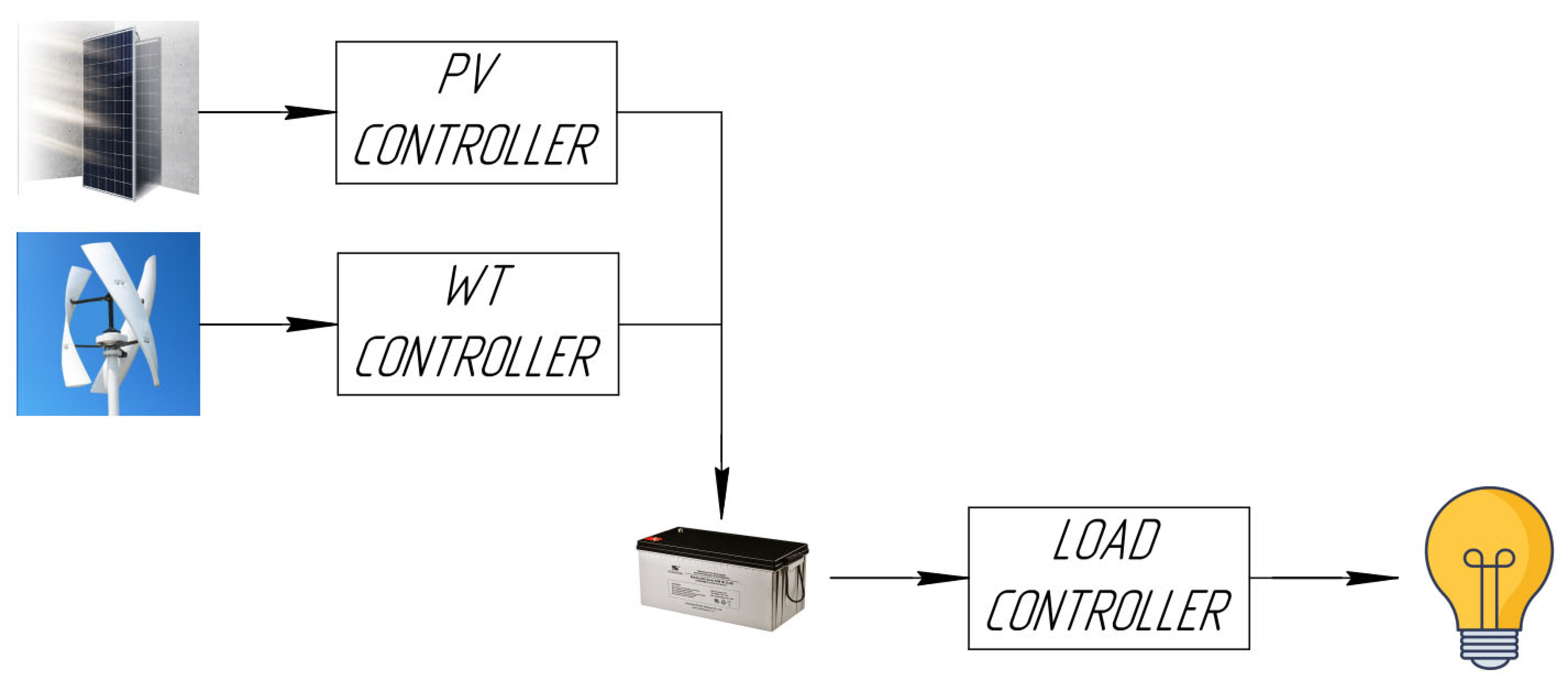
In this paper, study of the influence of the input weather data temporal resolution on a hybrid off-grid system is carried out for layout and reliability. The system under consideration (scheme is shown in Figure 1) consists of PV, WT and BES. In this study, an analysis of the reliability dependence of different off-grid supply system layouts on temporal resolution meteorological data obtained from Alpine weather stations (Switzerland) is carried out. The main criteria for evaluating the efficiency of each configuration version are the Reliability of Power Supply (RPS), the Longest Duration of Operation Interruption (LD) and the Cost of the Configuration Equipment per Year (CCY). These parameters can be regarded as characteristics of economic (CCY) and technical (RPS and LD) efficiency of off-grid power supply systems. The presented criteria are well suited for optimising the selection of power supply system configuration versions for both the lowest cost and the highest reliability. The results of this paper could be used in the design field of stand-alone systems based on PV.

2. Methods

2.1. Model of the Power Supply System

The numerical model of the off-grid power supply system is based on the balance analysis of generated, consumed and stored energy.

2.1.1. Solar Panel

The power ($W_{SP}$, W) generated by PV [15] depends on solar irradiance ($I$, W/m²) and the temperature of the solar panel itself ($T_{SP}$, °C):

$$W_{SP}=P_{\mathrm{SP}}\times \frac{I}{I_{ref}}\times \left(1+K_T\times \left(T_{ref}-T_{SP}\right)\right),$$

(1)

where $P_{\mathrm{SP}}$ is PV name-plate power (W); $I_{ref}$—solar irradiance at standard testing conditions (1000 W/m²); $T_{ref}$—PV nominal operating temperature (°C); $K_T$ is PV temperature coefficient (1/°C). We assumed PV to be horizontal to obtain some output during most of the daytime, so used GHI data for $W_{SP}$.

The PV temperature is expressed [15]:

$$T_{SP}=T_{amb}+0.0256\times I,$$

(2)

where $T_{amb}$—ambient air temperature (°C).

Accordingly, the energy, ($E_{SP}$, J), that is generated by PV for a certain time period ($\mathsf{\Delta }t$, s) is expressed as:

$$E_{SP}=W_{SP}\times \mathsf{\Delta }t,$$

(3)

2.1.2. Wind Turbine

The power ($W_W$, W) generated by WT depends on the wind speed (V, m/s) and the incoming air flow density ($\rho$, kg/m³):

$$W_W=\{\begin{array}{c}0, \sqrt[3]{\frac{\rho }{{\rho }_{ref}}}V<V_{min} \\ P_W\times \left(\frac{\frac{\rho }{{\rho }_{ref}}\times V^3-V_{min}^3}{V_{ref}^3-V_{min}^3}\right), V_{min}\le \sqrt[3]{\frac{\rho }{{\rho }_{ref}}}V<V_{max}\\ P_W\times \left(\frac{V_{max}^3-V_{min}^3}{V_{ref}^3-V_{min}^3}\right), V_{max}\le \sqrt[3]{\frac{\rho }{{\rho }_{ref}}}V \end{array},$$

(4)

where $P_W$ is the name-plate power of WT (W); $V_{min}$—WT start-up speed (m/s); $V_{max}$ is the cut-out speed of the WT (m/s); $V_{ref}$ is the nominal speed of the incoming air flow (m/s); ${\rho }_{ref}$ is the density of the incoming air flow under normal conditions (1.29 kg/m³).

The density of the incoming air flow depends on atmospheric pressure ($p$, Pa) and air temperature ($T_{amb}$, K) according to the Mendeleev–Clapeyron law:

$$\rho =\frac{p\times m_0}{R\times T_{amb}},$$

(5)

where $m_0$ is the molar mass of air (0.029 kg/m³);$R$—the universal gas constant (8.314 J/(mol × K));

Accordingly, the energy ($E_W$, J), which is generated by WT for a certain time period, ($\mathsf{\Delta }t$, s) is expressed as the follows:

$$E_W=W_W\times \mathsf{\Delta }t,$$

(6)

2.1.3. Battery Energy Storage

The energy ($E_B^C$, J) that could be stored in BES or taken from it (depending on the sign of the calculated value) is expressed on the basis of the values calculated by Equations (3) and (6):

$$E_B^C=(E_W+E_{SP})\times \mathsf{\eta }-\mathsf{\Delta }t\times W_N,$$

(7)

where $\mathsf{\eta }$ is the complex efficiency factor of energy converters; $W_N$ is the power of the energy consumer (W).

Energy ($E_B$, J), which is stored in the battery [15]:

$$E_B=\left(1-\sigma \right)\times E_B^{t-\mathsf{\Delta }t}+E_B^C,$$

(8)

where $E_B^{t-\mathsf{\Delta }t}$—the energy stored in BES at the previous iteration (J); $W_N$—the load (W); $\sigma$ is the degree of BES self-discharge for $\mathsf{\Delta }t$.

The maximum energy stored in the battery ($E_B^{max}, \mathrm{J}$) could be given by a polynomial dependence on temperature ($T_B$, °C) [16]:

$$E_B^{max}=E_B^{inst}\times (a_B\times T_B^2+b_B\times T_B+c_B),$$

(9)

where $a_B, b_B, c_B$—individual coefficients for different types of BES; $E_B^{inst}$ is BES installed capacity (J).

The energy stored in BES during charging is limited by the acceptable charge current. Accordingly, the maximum possible energy ($E_B^{C\_max}$, J), which could be stored in the battery during charging during the time interval $\mathsf{\Delta }t$, could be expressed as follows:

$$E_B^{C\_max}=k_C\times \mathsf{\Delta }t\times E_B^{inst},$$

(10)

where $k_C$ is a coefficient reflecting the battery charging rate. BES life is determined by the number of discharge cycles (LT), after which the actual battery capacity would decrease by 20% [16]. The dependence of LT on the battery State of Charge (SoC) could be given by a polynomial dependence [17]:

$$LT=a_K\times {\left(1-SoC\right)}^3+b_K\times {\left(1-SoC\right)}^2+c_K\times \left(1-SoC\right)+d_K,$$

(11)

where $a_K, b_K, c_K, d_K$ are individual coefficients for different types of BES.

Accordingly, the portion of the service life (ULT), that will be consumed as a result of the discharge process:

$$ULT=\frac{1}{LT},$$

(12)

2.1.4. Calculation Algorithm

The main criteria for the health of the power system are such indicators as the $LD$ and the $RPS$. The letter is taken as the ratio of the time during which the power was supplied ($t_p$, s) to the total time considered in the calculation ($t_f$, s):

$$RPS=\frac{t_p}{t_f},$$

(13)

$t_f$ is expressed as:

$$t_f=N\times \mathsf{\Delta }t,$$

(14)

where $N$—the number of time intervals.

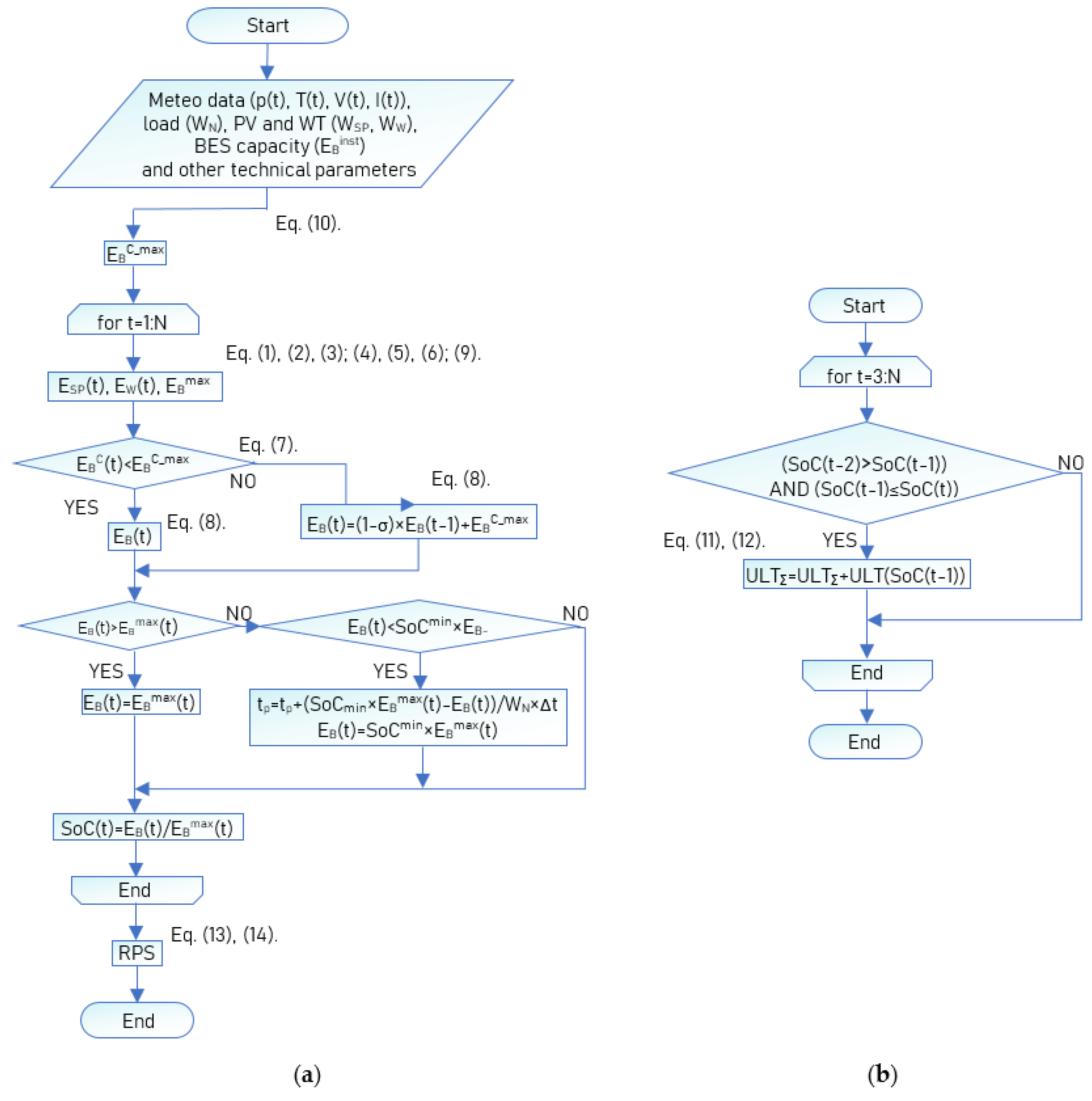
Algorithms for calculating these parameters and SoC depending on the time, as well as the part of BES life ($UL{T}_{\mathsf{\Sigma }}$), which will be consumed during the operation of BES during the estimated period of time, are represented in Figure 2.

The calculation process is reduced to obtain the BES SoC profile for each configuration version. Then, the RPS and LD can be estimated accordingly. The process of analysing the BES SoC at each point in time is divided into several steps:

• Calculation of the difference between generated and consumed energy
• The result is summing to the energy stored in the accumulator (at the previous step of the “for” cycle). At the same time, no more energy can be stored in the BES than the maximum possible energy, storing during the calculation time interval (calculated by Equation (10))
• The BES SoC is correcting to the maximum (minimum) permissible value (if the BES SoC together with the stored (withdrawn) energy is higher (lower) than the permissible SoC value at the previous step of calculation)

Additionally, on the basis of BES SoC profile analysis its service life can be estimated. This process is based on finding the BES SoC (throughout the calculation time interval) to which it has been discharged—each process of discharging the BES leads to a decrease in its lifetime by a certain amount (can be estimated by Equations (11) and (12)).

2.2. Initial Data

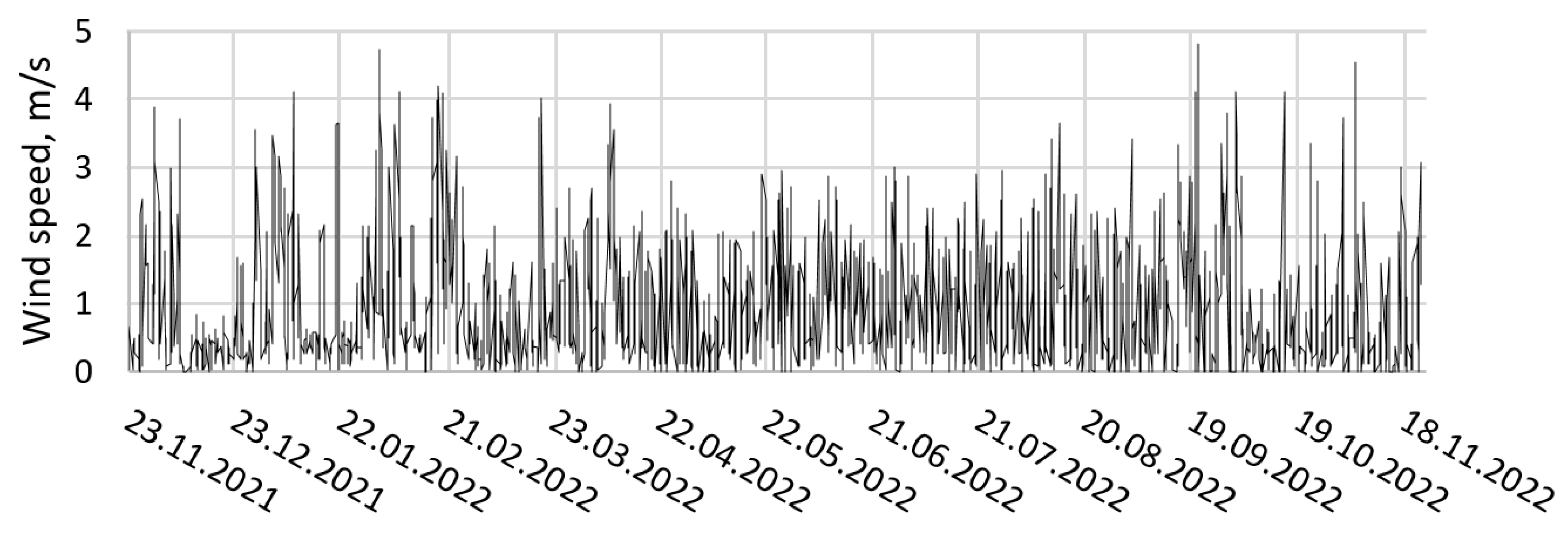
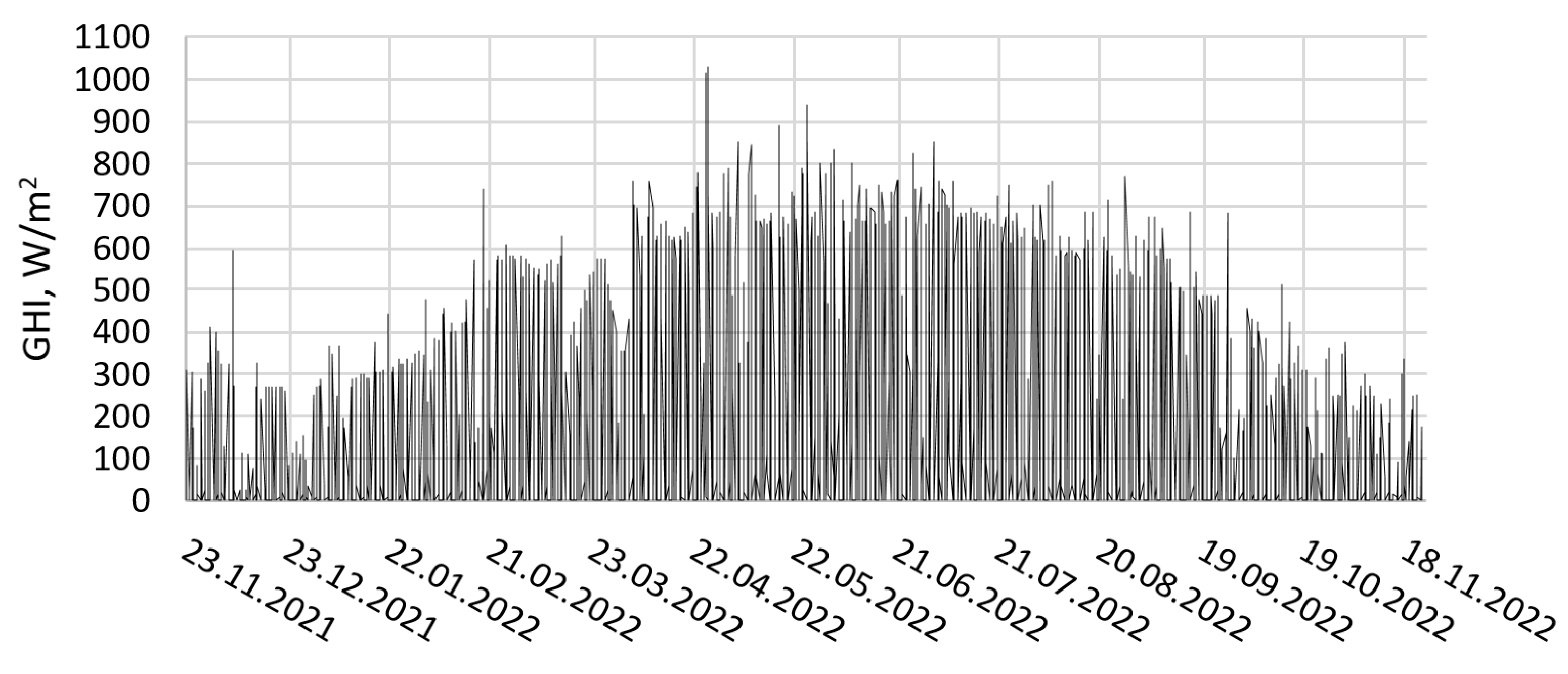
2.2.1. Weather Data

We used the meteorological data for the time period from 23 November 2021 to 22 November 2022 of the weather stations located in the Alps (see Supplementary Materials). The meteorological data of the average wind speed, solar irradiance (GHI), air temperature and atmospheric pressure were used. Information about stations is represented in

Table 1. Information about weather stations.

Station ID	Altitude	Location	Coordinates
47647	1700 m	Les Masses, Eremans, Switzerland	46.176, 7.389
23005	1830 m	Ze Hischinu, Staldenried, Switzerland	46.223, 7.901
39352	1830 m	Rosswald, Switzerland	46.305, 8.044

.

Weather data of the average wind speed and GHI for station 23005 are represented in Figure 3 and Figure 4, respectively. Weather data for all stations are represented in Supplementary Materials.

In this work, different weather data temporal resolutions were used:

• For 23 November 2021–22 November 2022: 30 min, 1 h, 2 h, 3 h, 4 h.
• For 24 August 2022–22 November 2022: 5 min, 10 min, 15 min, 20 min, 30 min, 1 h, 2 h, 3 h, 4 h.

2.2.2. Characteristics of the Power Supply System Equipment

A monitoring system with $W_N$ = 150 W is taken as an energy consumer. The sets of parameters varied in the calculation and are represented in

Table 2. Power system parameters.

Parameters	Values
The ratio of the installed capacity of solar panels to the total installed capacity, SWR 1	(0–1, step 0.1)
SoCmin	(0.2–0.8, step 0.2)
Total installed capacity, WΣ	(10–26, step 2) × WN, W
BES Capacity, EBinst	(0–10, step 0.5) × WΣ, W×h

¹ PV installed capacity is expressed as SWR×W_Σ, and WT as (1 − SWR) × W_Σ.

.

When calculating, various types of BES are considered: LiFePO4 SLPO12-200, AGM ML12-200, gel MLG12-200. The data on the dependence of the service life on the depth of discharge and the dependence of the battery capacity on temperature were converted into dependences convenient for analysis Figures S1–S4. The polynomial coefficients (according to Equations (9) and (11)) are represented in

Table 3. BES coefficients of polynomial dependencies and specific unit costs.

BES Model	${\mathit{a}}_{\mathit{K}}$	${\mathit{b}}_{\mathit{K}}$	${\mathit{c}}_{\mathit{K}}$	${\mathit{d}}_{\mathit{K}}$	${\mathit{a}}_{\mathit{B}}$	${\mathit{b}}_{\mathit{B}}$	${\mathit{c}}_{\mathit{B}}$	Cost, $/(A × h)
SLPO12-200	0	12,857	−25,286	15,429	−7 × 10−5	75 × 10−3	0.86	6.66
ML12-200	0	4428	−7042	2864				2.43
MLG12-200	0	4000	−6700	3450				2.70

. In general, the degree of self-discharge has a complex dependence on BES temperature, but to simplify calculations, for the considered 4-h time intervals for all BES models, it was taken as $\sigma$ = 0.4 × 10⁻³.

The costs of these BES models are represented (in specific units) in Table 3.

Data on cost and main technical characteristics of PV (using the example of HVL-390/HJT) and WT (using the example of ROSVETRO FX-1000) are represented in

Table 4. Information about power sources.

Power Source	Lifetime, Year	Cost, $/W
PV	30 years	0.82
WT	20 years	2.99

.

PV nominal operating temperature $T_{ref}$ = 38.8 °C and temperature coefficient $K_T$ = 2.85 × 10⁻³ 1/°C. WT start-up speed $V_{min}$ = 2 m/s, cut-out speed $V_{max}$ = 13 m/s and nominal speed of the incoming air flow $V_{ref}$ = 11 m/s.

The efficiency factor of converter and controller devices is assumed to be $\eta$ = 0.95.

The uncertainty associated with the power supply system components costs should be noted—the price difference between similar PV can reach 30%; WT—80%; BES—50%. In particular, unit cost changing due to the scaling of technical characteristics was not taken into account. The uncertainty associated with weather data should be considered: data averaged for the presented temporal intervals were not used, but the data measured once during these temporal intervals.

3. Results

As a result, a total of 24,948 variants of the power supply system were modelled based on weather data for each variant of temporal resolution and for each weather station. For the convenience of analysing such volumes of data, it is necessary to use methods of statistical data processing. Thus, the results of numerical modelling will be presented in the form of box-plots (diagrams). The boundaries of the box are the first and third quartiles; the line in the middle of the box is the median; the cross indicates the arithmetic mean. The whisker ends are the edges of a statistically significant sample. Outliers are not shown.

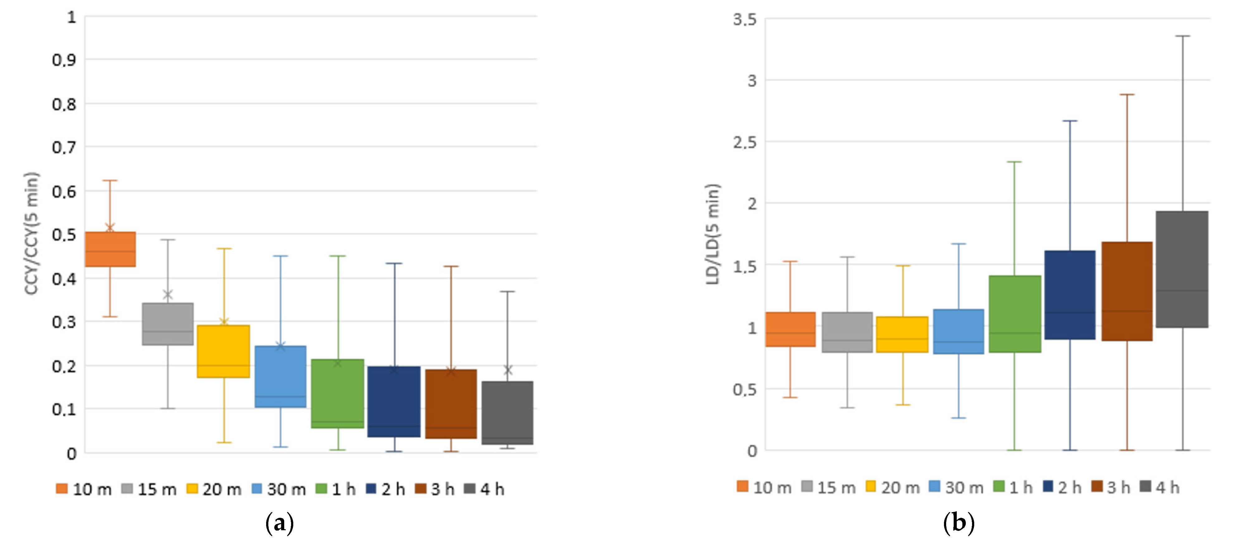
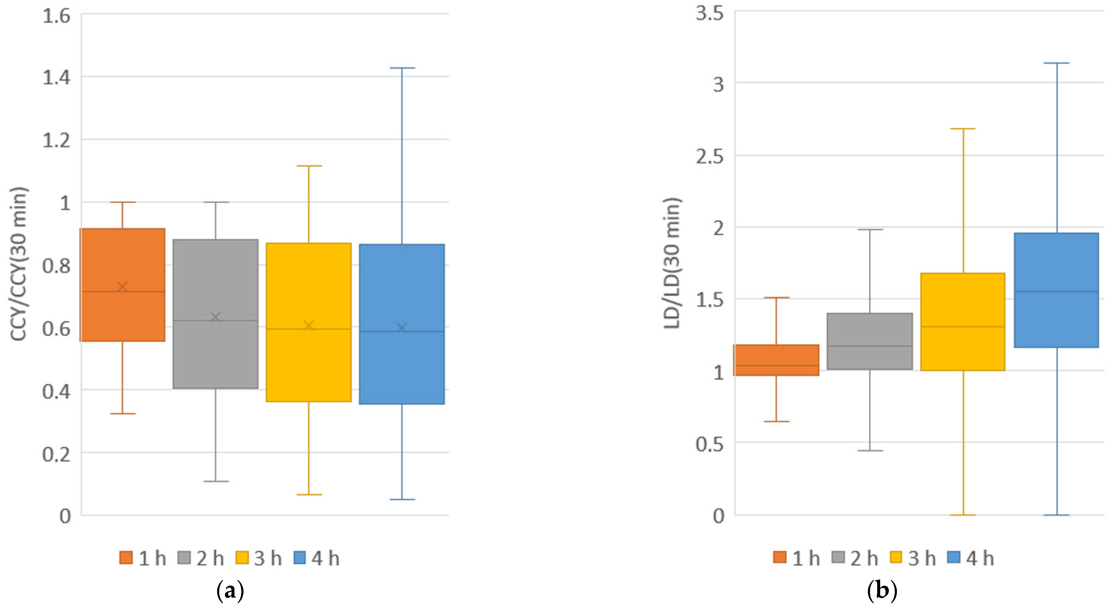
Figure 5a and Figure 6a show CCY at different temporal resolutions normalised by the CCY at 5 min and 30 min, respectively (for 3-month and annual datasets), for temporal resolution for station ID 23005. An increasing cost trend when refining the meteorological data temporal resolution is observed for both datasets. However, at the same time, the data scatter increases and generates the presence of configurations with overestimated CCY. Moreover, with a significant refinement of the temporal resolution, the growth rate also increases: the transition from 15 min temporal resolution to 10 min increases CCY by an average of 44% for 3-month datasets, and the transition from 10 min to 5 min temporal resolution by 92%. Such a significant cost increase (with higher temporal resolution of weather data) is due to a greater number of charge/discharge cycles (the number of which determines the lifetime of BES) during the simulation period.

Figure 5b and Figure 6b show the diagrams of LD at different temporal resolutions normalised by the LD at 5 min and 30 min, respectively, for temporal resolution for station ID 23005. There are slight differences between the results obtained at 10, 15, 20 and 30 min temporal resolutions for the 3-month dataset. However, a further decrease in the weather data resolution (1–4 h for both datasets) leads to overestimation of the LD results (compared to the calculation based on the data closest to real conditions). This also leads to a consistent increase in the scatter of the results, as the temporal resolution decreases. For other weather stations, similar results were obtained, so those are not shown.

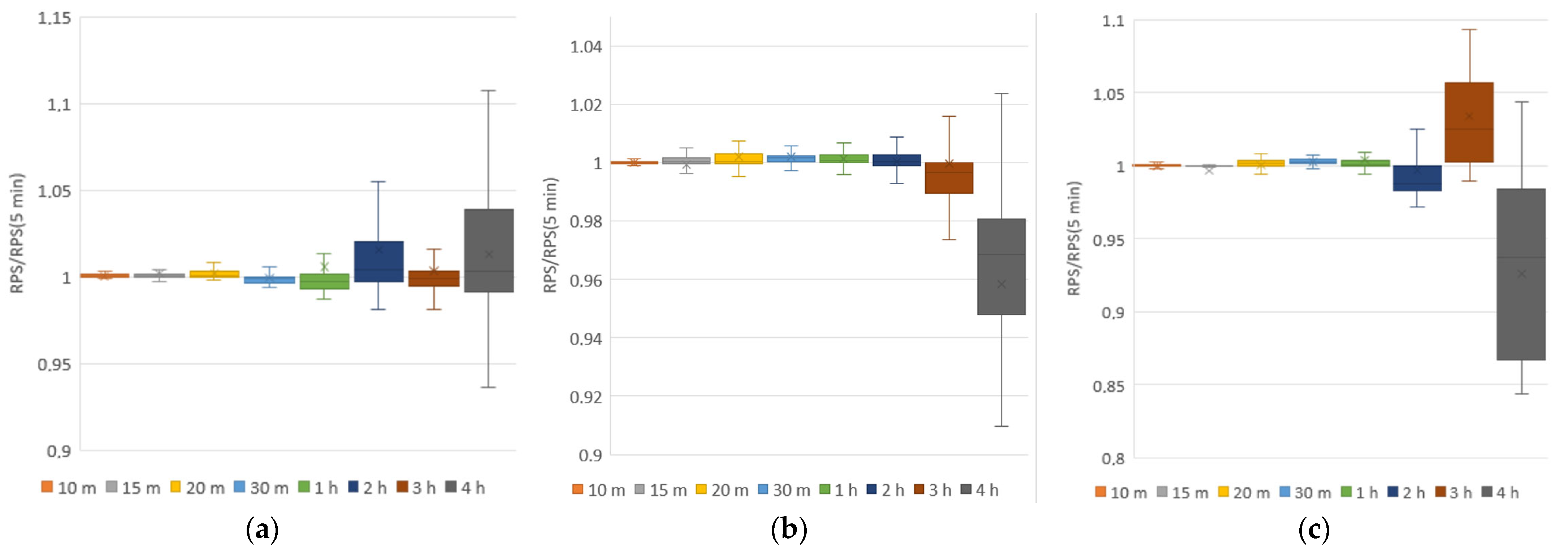
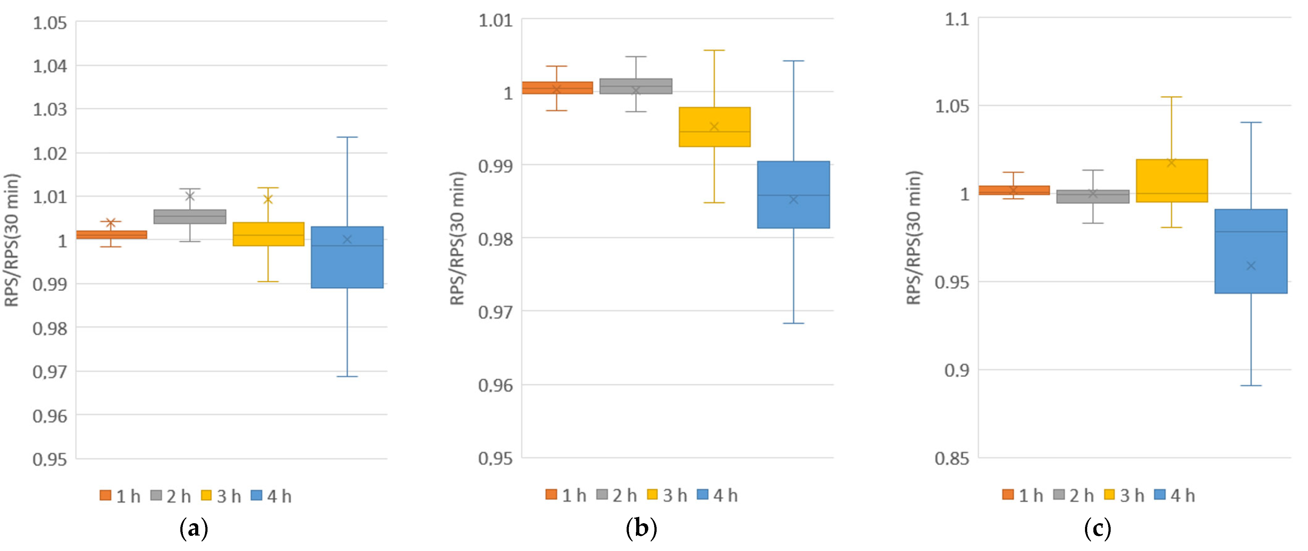
Diagrams of the RPS at different time resolutions normalised by RPS at 5 min and 30 min (for 3-month and annual datasets, respectively) temporal resolution are presented in Figure 7 and Figure 8 for all weather stations considered. The difference between the results obtained from 10 min to 1 h (from 1 to 2 h) temporal resolutions and those obtained at 5 min (30 min) is within 3% for most configurations of all three weather stations for 3-month datasets (1-year datasets). Noteworthy, the 3 h temporal resolution allows more accurate RPS estimation than the 2 h resolution for both datasets (according to the calculation results based on weather data from station 23005). At the same time, the results of calculations based on data from weather station 23005 show a clear trend towards overestimation of RPS when using less accurate weather data. The results of calculations based on data from weather station 39352, on the contrary, show an underestimation. The results obtained from the data of station 47647 also tend to underestimate RPS when using coarse temporal resolution (except for 3 h temporal resolution—it causes overestimation of RPS).

Thus, the RPS independence from the weather station location within the weather data temporal resolution from 5 min to 1 h is established for 3-month datasets. However, when coarser temporal resolutions (2–4 h for both datasets) are used, the RPS dependences specificity for each of the three weather stations are observed. Additionally, at first glance, it may seem that the calculation results by 4 h weather data differ significantly from the results by the more accurate weather data temporal resolution. However, this is just a visual effect—50% of the results have a difference in the range of 5% (for 1-year) and 10% (for 3-month) from the results of calculation by the most accurate temporal resolution, and there is no statistically significant difference.

4. Discussion

There are quite certain trends in the dependence of the calculation results of the main characteristics of the power supply system performance and its cost on the reduction of the weather data temporal resolution (relevant both for 3-month and 1-year data sets as the temporal resolution decreases):

• Underestimation of CCY
• Overestimation of LD

Analysis of RPS dynamics with decreasing temporal resolution provides no such unambiguous results. On the one hand, for 3-month datasets, using data with temporal resolution from 10 min to 1 h leads to results insignificantly different from those obtained with 5 min data (difference less than 3%). The same is valid for annual datasets: using time-resolved data at 1 and 2 h leads to results insignificantly different from those obtained with 30 min data. However, on the other hand, there is no definite regularity in the influence on RPS of 2, 3 and 4 h temporal resolutions: the dependence has an individual character for each of the three meteorological stations. There is also no results dependence on the location of the weather station.

RPS experiences minimal changes with a significant increase of temporal resolution (as in [12,13]). However, at the same time, the CCY exhibits an exponential growth character, which does not unambiguously determine the most optimal weather data temporal resolution for the power supply system design process (there is no estimate of the energy supply system cost in [13,14]). It is caused by an increase in the number of charge/discharge cycles of the BES during the calculation period, which leads to its more frequent replacement. In [10], the cost of a PV system depending on the temporal resolution is investigated, but without taking into account the lifetime limitation of BES. This leads to results that are opposite to ours—the difference in cost decreases when the temporal resolution is refined. Thus, it is worth noting the importance of considering the BES cycling influence on its service life in the off-grid power supply system model.

Thus, when analysing the performance of a particular configuration by RPS (with a sufficient degree of consistency with the actual operating conditions) it is allowed to use weather data with a temporal resolution of up to 1 h (including). However, to determine the optimal temporal resolution for CCY estimation, further work is needed to analyse the behaviour of CCY when using a temporal resolution of less than 5 min.

The efficiency analysis results of the same off-grid power supply system configuration variants are different depending on the location and the weather data temporal resolution. The basic economic and technical characteristics of configuration (1-year data, LiFePO4 SLPO12-200, SoC_min = 0.2, SWR = 1, W_Σ = 3 kW, E_B^inst = 6 kW × h), for example, are shown in the

Table 5. Characteristics of configuration.

Station ID	CCY, $/Year	RPS	LD, Days
47647	341	0.963	0.623
23005	324	0.981	0.617
39352	329	0.978	0.725

.

It was found inexpedient to use hybrid power supply systems in this area (Alps), because the wind speed is not enough for effective WT use (according to each of three weather stations). Despite this, it was also found that the difference in the calculation results relative to the change of the basic economic and technical characteristics (when varying the temporal resolution of weather data) is insignificant depending on the location of the weather station.

5. Conclusions

In this paper, the process of analysing the dependence of technical and economic parameters (reliability of power supply, cost of the configuration equipment per year, longest duration of operation interruption) of the power supply system on the weather data temporal resolution was presented. We simulated 24,948 different configurations (as a function of installed power, installed battery energy storage capacity, allowable minimal battery state of charge, power ratio between installed PV and wind turbines) for different temporal resolutions of weather data (5, 10, 15, 20, 30 min, 1, 2, 3, 4 h) obtained from three high-altitude alpine weather stations. Then, the results obtained for the same configurations, but different temporal resolutions, were compared with each other.

As a result, it was found inexpedient to significantly refine the weather data temporal resolution for the estimation of RPS—it is sufficient to use weather data with a temporal step less than 1 h; the exponential growth character of configurations cost with increasing temporal resolution; and the overestimation of the longest duration of operation interruption value with decreasing temporal resolution. In general, we recommend using 30 min resolution.

Among other things, it was found that PV-only power supply systems have proven to be the most productive and cheapest (per year) for the alpine highlands. The installation of hybrid power supply systems based on PV and WT both turned out to be impractical in the alpine highlands. Hybrid systems proved to be less productive and more expensive than PV-only systems in this region.

References

- Olabi, A.G.; Abdelkareem, M.A. Energy storage systems towards 2050. Energy 2021, 219, 119634. [Google Scholar] [CrossRef]
- IRENA. Off-Grid Renewable Energy Statistics 2021; International Renewable Energy Agency: Abu Dhabi, United Arab Emirates, 2021. [Google Scholar]
- IEA; IRENA; UNSD; World Bank; WHO. Tracking SDG 7: The Energy Progress Report. 2022. Available online: https://www.worldbank.org/en/topic/energy/publication/tracking-sdg-7-the-energy-progress-report-2022 (accessed on 23 November 2022).
- Akerboom, S.; Botzen, W.; Buijze, A.; Michels, A.; van Rijswick, M. Meeting goals of sustainability policy: CO2 emission reduction, cost-effectiveness and societal acceptance. An analysis of the proposal to phase-out coal in the Netherlands. Energy Policy 2020, 138, 111210. [Google Scholar] [CrossRef]
- Drozdova, I.v.; Alievskaya, N.v.; Belova, N.E. Problems and Prospects for the Development of the Arctic Zone of the Russian Federation. Lect. Notes Civ. Eng. 2021, 206, 137–143. [Google Scholar] [CrossRef]
- Sayed, E.T.; Wilberforce, T.; Elsaid, K.; Rabaia MK, H.; Abdelkareem, M.A.; Chae, K.J.; Olabi, A.G. A critical review on environmental impacts of renewable energy systems and mitigation strategies: Wind, hydro, biomass and geothermal. Sci. Total Environ. 2021, 766, 144505. [Google Scholar] [CrossRef] [PubMed]
- Loktionov, E.Y.; Sharaborova, E.S.; Shepitko, T.V. A sustainable concept for permafrost thermal stabilization. Sustain. Energy Technol. Assess. 2022, 52, 102003. [Google Scholar] [CrossRef]
- Sharaborova, E.S.; Shepitko, T.V.; Loktionov, E.Y. Experimental Proof of a Solar-Powered Heat Pump System for Soil Thermal Stabilization. Energies 2022, 15, 2118. [Google Scholar] [CrossRef]
- Asanov, I.M.; Loktionov, E.Y. Possible benefits from PV modules integration in railroad linear structures. Renew. Energy Focus 2018, 25, 1–3. [Google Scholar] [CrossRef]
- Chiang, M.Y.; Huang, S.C.; Hsiao, T.C.; Zhan, T.S.; Hou, J.C. Optimal Sizing and Location of Photovoltaic Generation and Energy Storage Systems in an Unbalanced Distribution System. Energies 2022, 15, 6682. [Google Scholar] [CrossRef]
- Salameh, T.; Kumar, P.P.; Olabi, A.G.; Obaideen, K.; Sayed, E.T.; Maghrabie, H.M.; Abdelkareem, M.A. Best battery storage technologies of solar photovoltaic systems for desalination plant using the results of multi optimization algorithms and sustainable development goals. J. Energy Storage 2022, 55, 105312. [Google Scholar] [CrossRef]
- Tang, R.; Abdulla, K.; Leong, P.H.; Vassallo, A.; Dore, J. Impacts of Temporal Resolution and System Efficiency on PV Battery System Optimisation. In Proceedings of the Asia-Pacific Solar Research Conference, Melbourne, Australia, 5–7 December 2017. [Google Scholar]
- Hauck, B.; Wang, W.; Xue, Y. On the model granularity and temporal resolution of residential PV-battery system simulation. Dev. Built Environ. 2021, 6, 100046. [Google Scholar] [CrossRef]
- Jaszczur, M.; Hassan, Q.; Teneta, J. Temporal load resolution impact on PV/grid system energy flows. MATEC Web Conf. 2018, 240, 04003. [Google Scholar] [CrossRef]
- Kumar, P.P.; Saini, R.P. Optimization of an off-grid integrated hybrid renewable energy system with various energy storage technologies using different dispatch strategies. Energy Sources Part A Recovery Util. Environ. Eff. 2020, 42, 1–30. [Google Scholar] [CrossRef]
- Saldaña, G.; Martín JI, S.; Zamora, I.; Asensio, F.J.; Oñederra, O.; González-Pérez, M. Empirical calendar ageing model for electric vehicles and energy storage systems batteries. J. Energy Storage 2022, 55, 105676. [Google Scholar] [CrossRef]
- Collath, N.; Tepe, B.; Englberger, S.; Jossen, A.; Hesse, H. Aging aware operation of lithium-ion battery energy storage systems: A review. J. Energy Storage 2022, 55, 105634. [Google Scholar] [CrossRef]