1. Introduction
Due to rapidly increasing global warming caused by the emission of greenhouse gases into the atmosphere from the burning of oil, gas and coal, there is a need for alternative technologies to satisfy the world’s energy demand by environmentally friendly technologies [
1]. In addition, because of increasing costs for oil, gas and wood, independence in the energy sector comes into focus. For example, electricity, which can be easily produced by renewable energy sources, may be the energy carrier of the future. Germany, which is dependent on imports of gas and oil, can only achieve sufficient independence through extensive electrification of all sectors and a strong expansion of renewable energy systems.
The energy that is theoretically available from renewable energy sources could easily meet the demand for energy in Germany [
2]. However, energy storage represents the biggest issue due to the typically diverging (fluctuating) energy demand compared to the supply. Germany’s low sun irradiance in winter leads to a high seasonal storage requirement. Hydrogen, due to its high energy density and unrestricted storage opportunities, could be a promising opportunity for covering the energy demand during this period. Hydrogen, when produced by renewable energy sources (RES), is seen as one of the most promising means of transforming the energy system in a climate-friendly way.
Due to high capital costs for hydrogen-based small-scale energy systems, both resource and cost efficiency are important factors for success, and it is important that the components are well suited to the respective application where the energy system shall be used. In addition, an analysis of how much self-sufficiency is possible with such a system may be of interest. A preceding simulation with input data which characterizes the application for determining the optimal component dimensioning can save resources and money. In particular, the lifetime of the components, which highly depends on the dimensioning, the component constellation and the control system, is an important factor for the system costs. Thus, a lifetime prediction model was integrated into the energy system model, which was designed for the analysis of the energy balance within one year. The energy system model was presented in detail in a previous paper [
3].
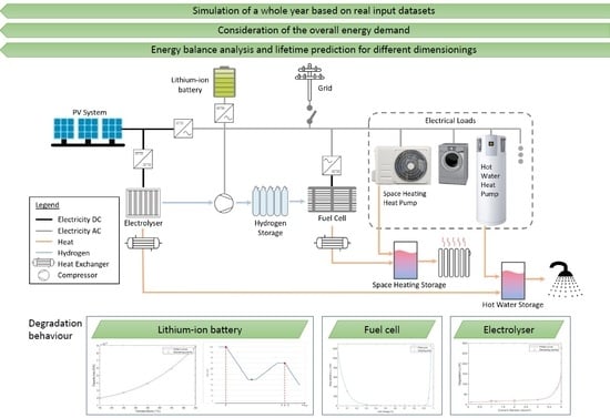
The energy system construction consists of a PV system which is the main energy source. It is oversized to ensure high excess energy production during summer, which is used for hydrogen production by an electrolyser (ELY). The hydrogen is compressed and stored for usage in a fuel cell (FC), where the hydrogen is reconverted to electricity on demand. The hydrogen system is used for long-term storage, while a lithium-ion battery (LIB) is used for short-term energy demand. An LIB can better deal with rapid load peaks compared to FCs and is therefore required to guarantee a high level of self-sufficiency. The heating system was also considered, as the focus was on ensuring the overall energy demand by PV. The waste heat of the FC was used inside the space heating system, while the waste heat of the ELY was used for the hot water heating demand. The remaining energy demands were met from electrical heat pumps. The energy system model was created in Matlab/Simulink [
4] and was designed for the analysis of a real data series over an entire year with a time resolution of 15 min. A representative dataset recorded in Switzerland in 2012 was used as household load profile [
5]. Irradiance and temperature profiles with a time resolution of one hour have been granted by German Weather Service (Deutscher Wetterdienst—DWD) [
6]. The data sets were recorded during 2015 in Wuerzburg (Germany).
The topic “hydrogen in energy systems” is presently attaining increasing interest in the research community. Such systems are analyzed at various levels and in several component constellations. Many modelling studies deal with dynamic real-time operation and control, examining relatively small time scales of a few hours, a day, or up to two weeks, such as [
7,
8,
9,
10]. Certain component constellations have been examined quite often, such as hybrid energy systems designed for wind power as the only energy source [
11]; others assume hydrogen as the only kind of energy storage [
12]. In our paper, a more holistic approach to an energy system was chosen, which also takes into account heating requirements and consists of a hybrid solution with hydrogen and LIB as energy storages. This modelling approach intents to provide support for the design of future energy systems of this type. In this context, a simulation designed for an entire year was relevant in order to consider the seasonal dependency of energy production and energy demand. The integration of real input data along with high-resolution processing has been rarely used thus far. In addition, the design of an extensive control system by Simulink is also featured. As a result, this model offers some advantages, such as a higher resolution for more meaningful analysis and design statements, the delimitation of the use case and the integration of arbitrary additional objects of investigation—compared to other modeling tools such as Homer Energy [
13], ReMOD-D [
14] or TRNSYS [
15].
In the literature, research has been carried out on this topic. For example, in [
12], the authors presented a hybrid energy system including renewable energy sources (RES) as an energy supply, an alkaline ELY, a proton exchange membrane fuel cell (PEMFC) and a hydrogen storage system. They focused on the analysis of the system’s dynamics with the aim to improve self-sufficiency by reducing grid interaction. However, an LIB and a heating system have not been considered. Due to the lack of short-term energy storage, hydrogen storage was used to store the hydrogen produced by the ELY within one day, and directly reconverted the hydrogen by the use of an FC once the energy production with RES was less than the energy demand. In [
16], a Simulink model of an energy system consisting of a PV system, a PEM ELY and a hydrogen storage system was also presented. The model was created for the analysis of system dynamics and was therefore used for short-term analysis. However, it did not consider an FC and real load profiles. In [
8], a hydrogen-based energy system model created in Simulink was presented. The authors used a time horizon of 24 h with a focus on power management and control systems. They analyzed the suitability of a hydrogen-based energy system consisting of hydrogen as the only energy storage type for stand-alone systems. However, within the load profile used in this approach, rapid load peaks were neglected, which is not realistic. To guarantee a higher lifetime, rapid load peaks should not be solely covered by an FC [
17]; therefore, an additional LIB should be used, which reacts more quickly on rapid load peaks and is much more robust in terms of lifetime.
The lifetime prognosis parameters used in this research originate from literature research, from which various sources have been compiled. Based on the degradation values of different sources, we developed our own degradation curves to represent the degradation under certain influencing variables. Since the literature on lifetime analysis for ELYs and FCs contains limited examination, only a small amount of sampling points could be identified from different sources that describe the degradation under certain conditions. For example, in [
18], only the degradation of a PEM ELY at current densities of 1 A/cm
2 and 3 A/cm
2 was examined. Since the ELY in this model is operated based on fluctuating PV energy surpluses, the actual current density fluctuates significantly over the course of operation. Therefore, sampling points from various sources have been compiled as a result of the literature analysis in order to cover degradation values for the entire range of operation from 0 A/cm
2 to approx. 4 A/cm
2.
No literature could be found in which a lifetime analysis for an ELY was carried out as part of a simulation within a realistic application. In contrast, a simulation-based FC lifetime analysis was performed by Ms. Bonitz [
17]. The findings from her work serve as the base for estimating the lifetime of the FC in this research project. However, only the methodology has been adopted, since a degradation curve which is more compatible with the available sampling points was found and is used in this paper. For LIB lifetime prediction, much more research has already been carried out. The main task here was to find literature sources that followed a simulation-based approach and to identify key factors for lifetime estimation that could be reliably used by a modelling approach.
A combined lifetime analysis of all three components, ELY, FC and LIB, within an energy system has not yet been the subject of current research. Within the scope of this investigation, it is hoped to gain insights into mutual interdependency and effect. This research aims to show what kind of impact component sizing has on the lifetime of the system.
This paper is organised as follows:
Section 2 introduces the input data used for the model validation and describes its control scheme and system architecture. In addition, the background used for the lifetime prediction model is described within this section.
Section 3 describes various outcomes of parameter studies in terms of lifetime expectation for the main components and the energy balance.
Section 4 discusses the results of the findings and the strengths of the energy system model in combination with a lifetime prediction. Finally,
Section 5 concludes the findings.
2. Materials and Methods
2.1. Input Data
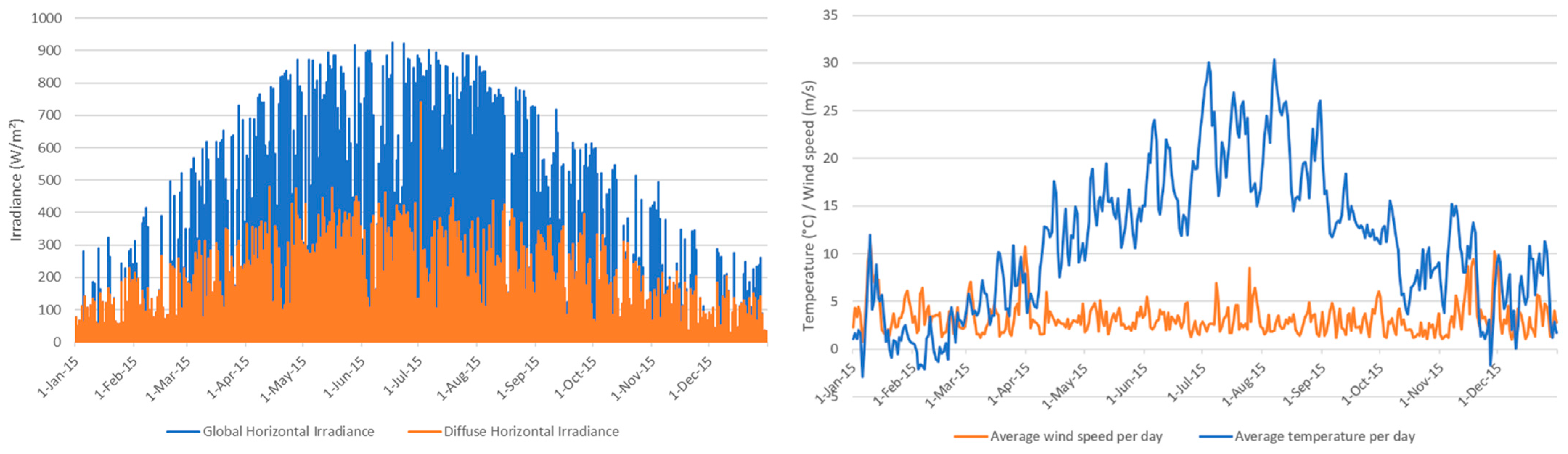
Figure 1 shows the weather data recorded from the DWD in the year 2015 as input for the simulation. The ambient temperature and wind speed trends are shown in
Figure 1 (right). The data have been averaged for each day to achieve a better visualisation of the trend. The temperature curve has an arithmetic mean of 11.07 °C and a standard deviation of 7.44 °C. The wind speed trend is used for calculation of the probable cell temperature of the PV modules to achieve more realistic PV energy yields. The wind speed has an arithmetic mean of 3.26 m/s and a standard deviation of 1.76 m/s. The curve of the global horizontal irradiance is shown in
Figure 1 (left).
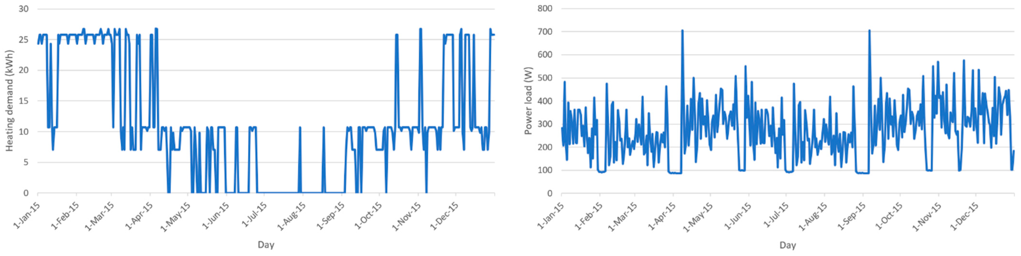
A synthetic heat demand profile was generated using the VDI 4655 standard, which provides reference load profiles of single-family and multi-family houses for the use of Combined Heat and Power (CHP) systems [
19]. By using an Excel tool created by Hessen [
20], which uses the reference load profiles from the VDI 6455 standard, a heating demand profile with a 15 min time resolution was generated. The generated heating demand profile depends on the actual ambient temperature within the time frame, which is given by the DWD for the selected year, 2015. The heating demand curve for the year can be seen in
Figure 2 (left). As can be seen, the demand ranges from 26.72 kWh per day (commonly during winter period) and 0 kWh (during summer period). For the year of simulation, a total heating demand of 4000 kWh (via an electrical heat pump), and an energy demand for hot water preparation in the amount of 1000 kWh, was assumed. The electrical load profile used for the simulation (
Figure 2 (right)) has a base load of around 100 W, an arithmetic mean of 268.96 W and a standard deviation of 119.85 W, which leads to an overall electrical energy demand of 2356.09 kWh. The base load is evident from time periods when residents were absent from their dwellings.
2.2. System Layout
This subsection qualitatively describes the overall hybrid energy system and main changes of some partial component models. The main model and a detailed explanation of the functions describing the partial component models are shown in a previous paper [
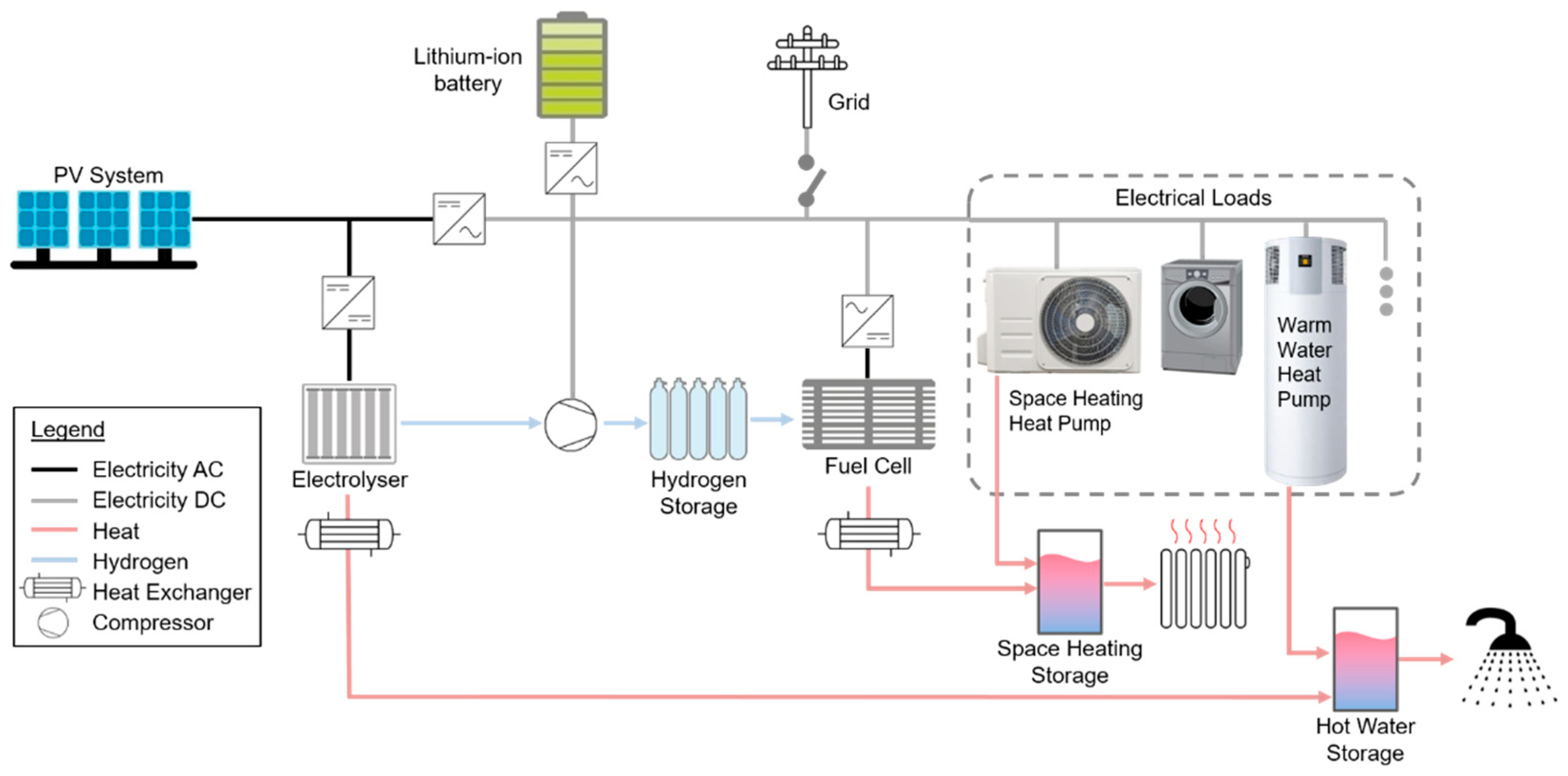
3]. The core elements of the energy system model are a fuel cell (FC), an electrolyser (ELY), a lithium-ion battery (LIB), a hydrogen storage tank and a PV system, as well as a newly added model for the heating system (especially the hot water heating system).
Figure 3 shows the architecture of the proposed energy system. The PV system serves as the main energy source. With an inverter, the captured solar energy can directly be used for the electrical loads in the household (direct consumption). Any surplus is initially stored in the LIB which is integrated on the AC side. A charge/discharge controller has been integrated between the LIB and the household’s grid. Energy stored inside the LIB is transferred back to the household grid via an inverter in the case of less energy production versus demand. If the LIB is fully charged and the PV system still generates surplus energy, the ELY is switched on and hydrogen is produced by the surplus energy. After passing a compressor, the hydrogen is stored inside the hydrogen tank. In case of high electricity demand in combination with low energy production and an empty LIB, the FC is switched on. The FC acts as an electricity supplier for electrical loads and is controlled based on the State of Charge (SoC) of the LIB. The LIB should have a remaining energy buffer when the FC is turned on, because load peaks are covered by the LIB. When the FC produces surplus energy which is not required for covering the energy demand, the LIB is recharged with this energy. The power level of the FC is adjusted when the LIB reaches predefined SoCs, such as those presented in the next section. A control algorithm via Simulink chart is used to control the energy flow. The principle of the control system used in this approach is the same as in the first paper [
3] and has already been described in detail in
Section 6 of this paper.
For every inverter within the energy system, an efficiency of 95% was assumed. For the LIB, a change and discharge efficiency of 95% was assumed, and for the PV system, constant losses of 10% were assumed, which consider pollution, conduction losses, etc.
Since the electrical efficiency of an ELY (67–82%) [
23] and an FC (36–45%) [
24] is relatively low, the overall system efficiency can be increased by considering the thermal efficiency (additional 52% for FC [
24]) and therefore using the waste heat inside the hot water heating or space heating system. Therefore, heat exchangers have been introduced into the model, which extract the heat generated inside the ELY and the FC. As the produced PV energy in combination with an LIB achieves a high self-sufficiency during midyear, the FC is predominantly used in winter, which coincidences with the heating period. Therefore, an integration of the waste heat generated by an FC into the space heating system is preferable. As small-scale PEMFCs typically operate at temperatures of around 60 °C, a transfer of the waste heat into the heating system is possible.
It was decided to use a Proton Exchange Membrane (PEM) ELY due to its advantages such as the intrinsic ability to cope with fast transient electrical power variations, which is especially important when fed by fluctuating renewable energies like PV in the designated use case [
25]. Moreover, they have, compared to other ELY types, lower operating temperatures and lower power consumption, and are therefore better suited for small-scale applications [
26]. Low-temperature PEM ELYs commonly operate between 50 °C and 80 °C, and have to be cooled in order to protect them against degradation caused by a temperature increase above 80 °C [
27]. The heat extracted from the ELY can be used as additional heat for the hot water heating system because ELYs are typically operating during summertime when space heating is not necessary. The residual heat demand is then covered by a hot water heat pump. Such a heat pump typically achieves water temperatures of around 65 °C maximum, while the temperature inside a hot water storage shall always exceed 50 °C. Because of an operating temperature of 50 °C to 80 °C, waste heat usage is possible.
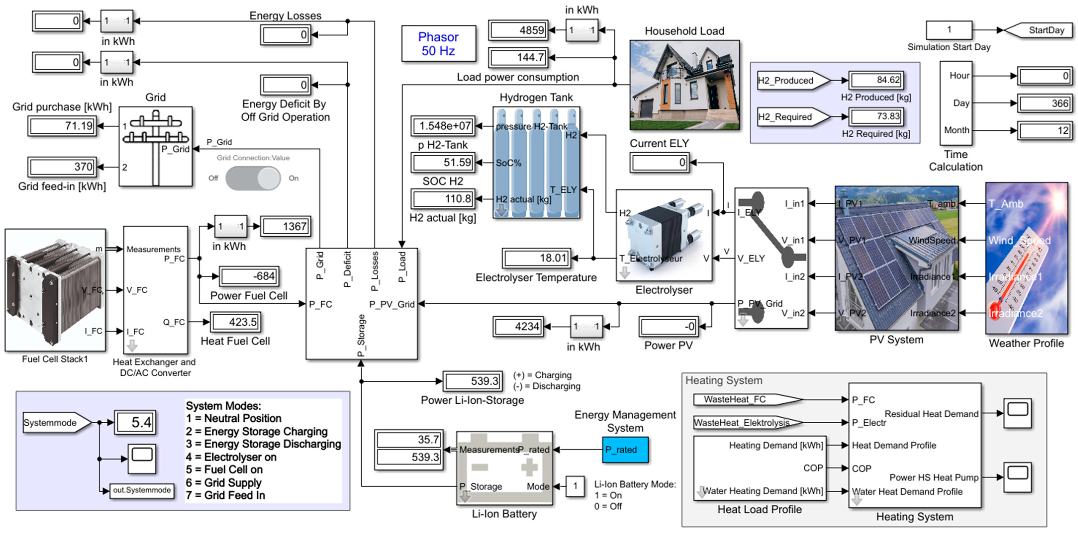
Figure 4 shows the overall energy system model created in Simulink. The Matlab/Simulink version R2021b was used.
2.3. Control Scheme
The control system is one of the most important parts of the energy system. It controls the energy flow of all components and ensures the coordination and collaboration of every component. It also has a high impact on the lifetime of the components, especially for the FC (hence the reason why great effort went into implementing a complex energy system). The schematic control procedure of the two main components, the FC and the ELY, will now be presented.
For the FC, a three-stage power adjustment which is based on the actual SoC of the LIB was implemented. The stages are as follows:
30% SoC →
45% SoC →
55% SoC →
70% SoC → FC switched off
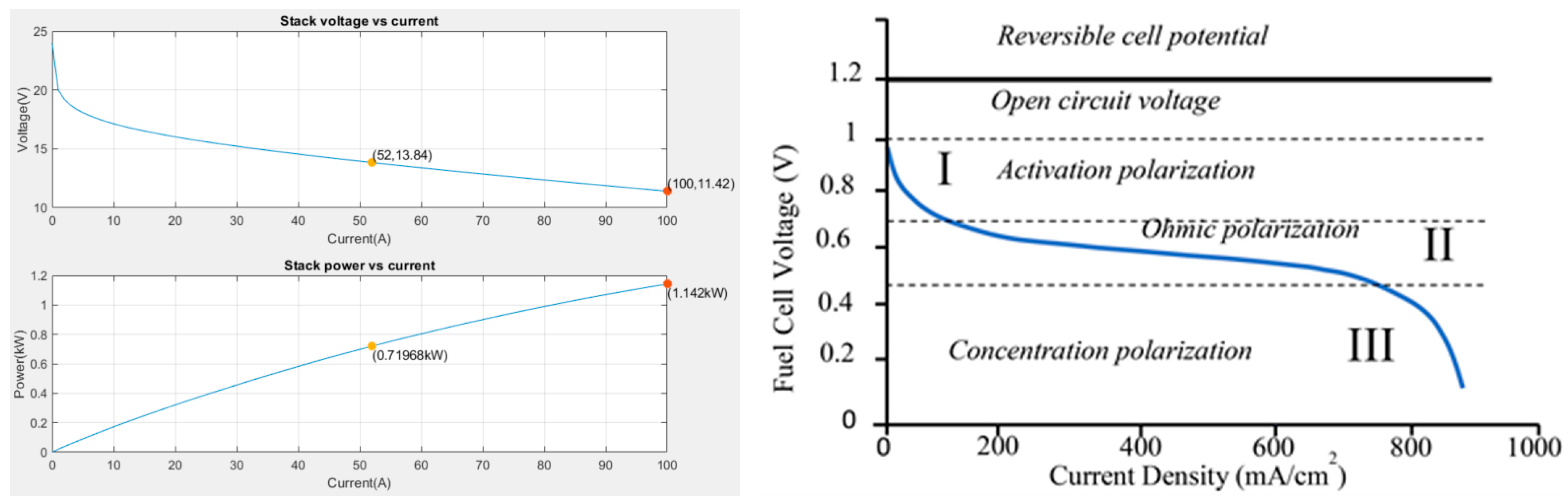
The plot generated by the Simulink “Fuel Cell Stack” block for an exemplary FC with a nominal power of 720 W (
Figure 5 (left)) in combination with a typical V-I curve of an FC (
Figure 5 (right)) shows that the FC still operates in operating range even at an FC power of
. The FC can only change the power stage every 15 min and changes the power level slowly; since rapid current changes affect the lifetime of an FC, fast changes should be prevented. In return, the LIB covers rapid load peaks; therefore, the LIB should always have enough energy buffer. This means that the FC switches on even before the LIB is completely empty. The LIB is charged by the residual energy delivered by the FC in case of consumption of energy lower than that produced by the FC, and as long as the SoC of the LIB does not reach a predefined state.
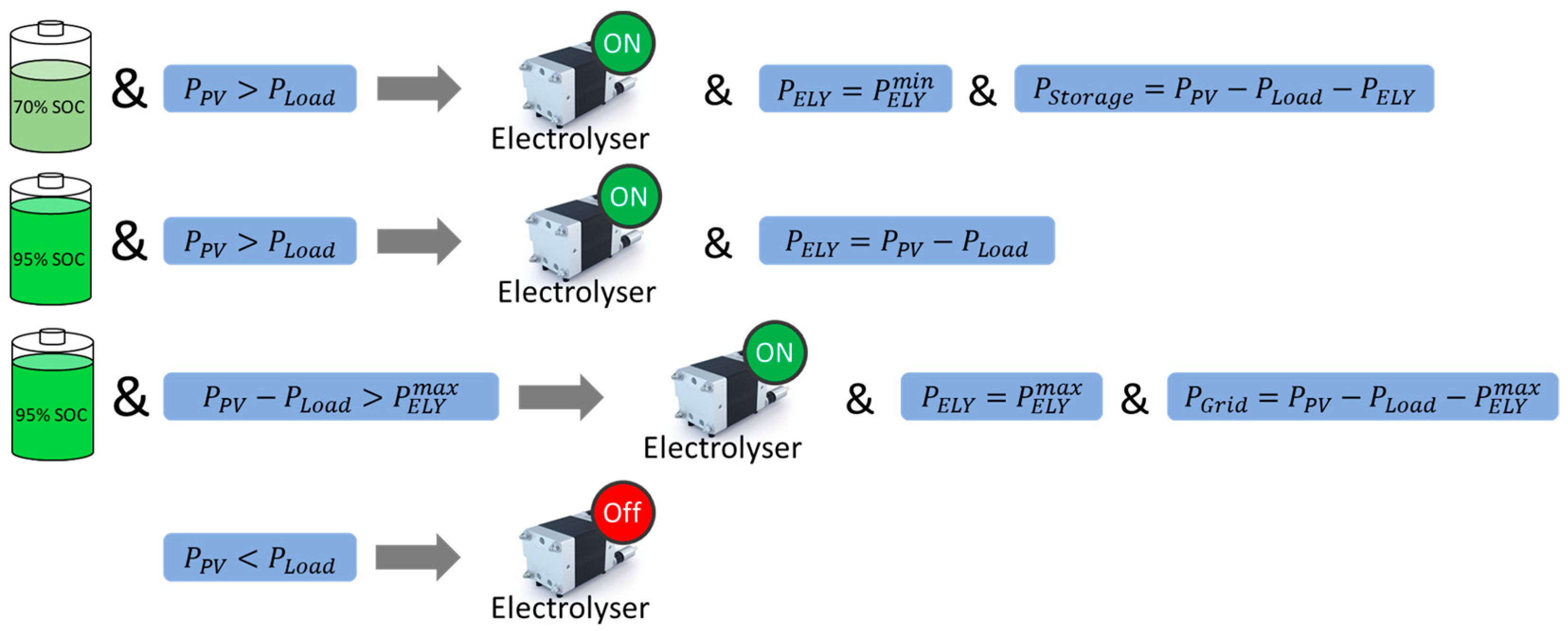
The ELY control is also based on the SoC of the LIB. The control scheme is shown in
Figure 6.
This leads to an operation occurring more often at low power. The lifetime of the ELY should not be highly influenced by operation at minimum power, as shown in
Section 2.4.3. Additionally, an operation at low operation power leads to more efficient hydrogen production. The hydrogen production is increased and the energy losses at off-grid operation also decrease by this type of control, because if the ELY first turns on as soon as the LIB is full of charge and then the surplus energy exceeds the minimum ELY operating power, this energy is wasted.
2.4. Lifetime Analysis
For a better evaluation of the component dimensioning in terms of resource usage, a lifetime analysis is meaningful. A different component size affects different component stresses as, for example, a larger LIB capacity means that the FC cannot operate efficiently because more PV energy can be stored in the short term, and as a second effect, the FC must not switch on that often. A simulation of such an energy system with integration of a lifetime analysis therefore enables a more meaningful implication, as the relations and impacts of the components are highly complex. Of note is that the lifetime of the ELY, the FC and the LIB, is highly influenced by operating conditions, the operating point and the control scheme. A simulation via Simulink enables an extensive analysis of these conditions.
After detailed literature research, lifetime prediction models for the three components, FC, ELY and LIB, have been developed. A targeted search was made for studies that can be used in a generalized manner, which estimate the service life with only a few but the most important input variables and with sufficient accuracy. In the next subsections, the lifetime prediction models and the methodology of integration into the energy system model will be presented.
2.4.1. Lifetime Prediction Model—Lithium-Ion Battery
The lifetime of the LIB is subdivided into cycle and calendar aging. Calendar aging typically leads to a capacity loss which is defined to be up to 20% until End of Life (EoL) [
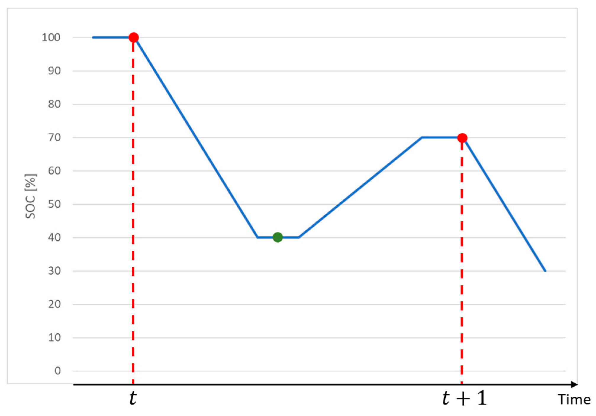
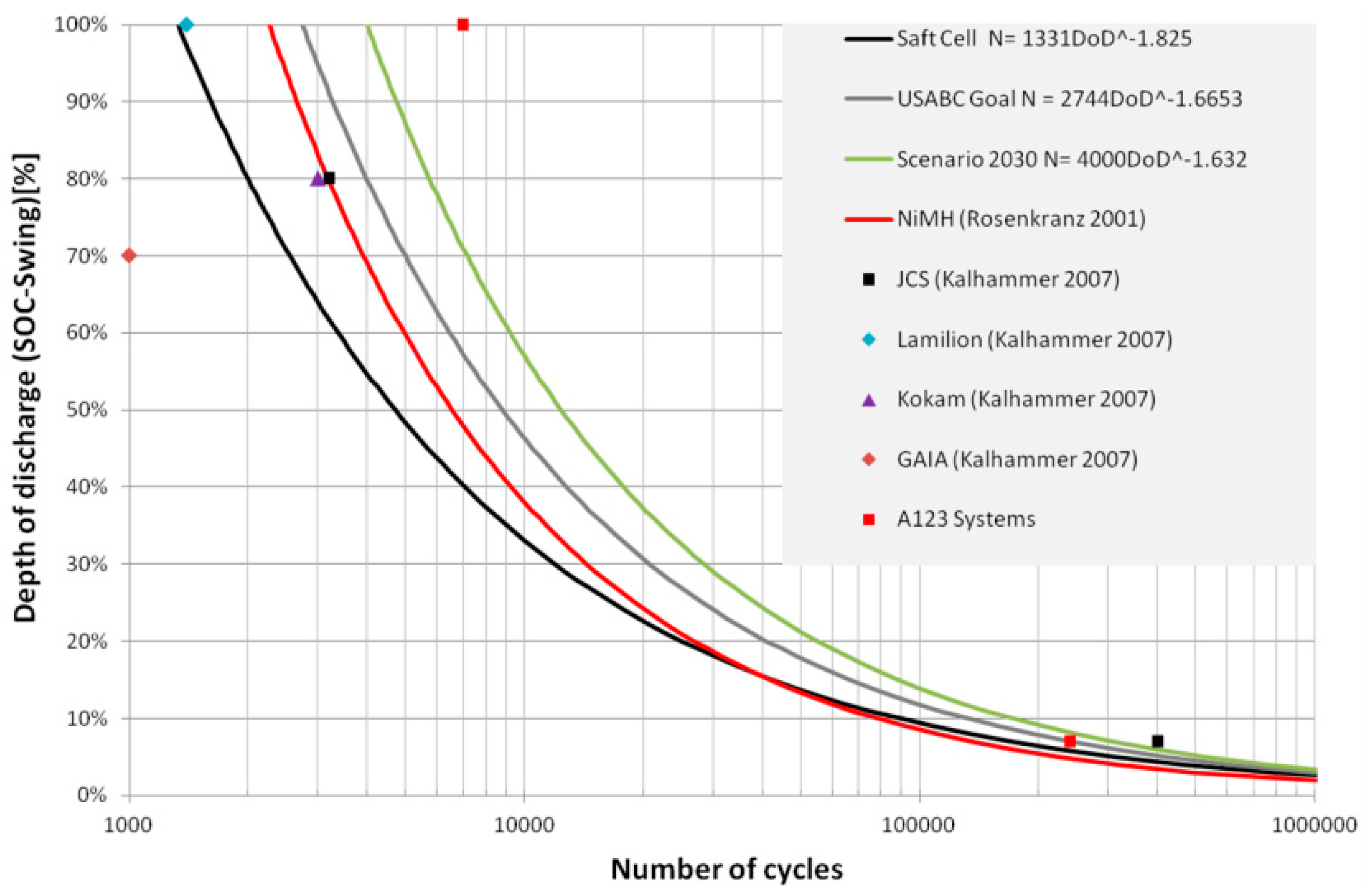
31]. In contrast, cycle aging is the share of aging that results from the use of the battery (repeated charging and discharging). The key factor influencing cycle aging is the Depth of Discharge (DoD), but the C-rate can also have an influence, particularly high C-rates. In the literature, calendar aging is defined by a maximum number of cycles which the battery can run until lifetime end, while the amount of cycles means full cycles where a battery is discharged from 100% SoC to the minimum permitted SoC, and then recharged to 100%. As batteries are typically used with applications where different cycles with different upper and lower SoCs occur, a Full Cycle Equivalent (FCE) has to be calculated for every partial cycle. When a minimum permitted SoC of 0% is assumed, a particular cycle from 100% SoC to 30% SoC and back to 100% would mean an FCE of 70%. An example for the calculation procedure of a more random cycle from 100% to 40% and back to 70% is shown in
Figure 7. Following Formula (3), this cycle would result in an FCE of 45%.
The partial cycle shown in
Figure 7 has a DoD of 60% (100% SoC–40% SoC). When assuming that actual LIBs follow the degradation curve of the U.S. Advanced Battery Consortium (USABC) in
Figure 8 obtained from Dallinger [
32], a DoD of 60% would result in a maximum of 6424 full cycles. This means that one full cycle would lead to a degradation of
. This degradation has to be multiplied by the previously calculated FCE of 45%, whereby the cyclic degradation of the partial cycle shown in
Figure 7 would be
.
For every partial cycle within the whole simulation time of 1 year, the previously shown procedure has to be performed. Therefore, Matlab was used. In the end, the degradation of every partial cycle has to be summed to obtain the overall degradation caused by DoD. In addition, the overall cycles within the year of interest are calculated by summing up the partial cycles. The standard deviation from calculating the full cycles by using our own approach with the FCE compared to the calculation via the standard procedure, where the full cycles are calculated by the outgoing energy and the overall LIB capacity, was 0.57. This proves that our own procedure is in good agreement with the standard procedure and can be used for the calculation of the partial cycle degradation. The calculated overall degradation caused by DoD characterizes the overall cycle aging. When this type of degradation reaches 100%, the EoL of the LIB is reached.
The C-rate as a second factor for the cycle aging has not been covered due to predominantly low C-rates occurring when used in a stationary application for a single household. The parameter study via simulation showed a maximum average charging C-rate of 0.1 and a maximum average discharge C-rate of 0.07, which is low compared to other use cases, such as in electric vehicles with fast charging functions. These C-rates may increase with higher resolution of the input data. However, a resolution of 15 min was chosen due to an excessive increase in simulation time, and due to missing input data with higher resolution for weather and heating demand.
The second type of aging, calendar aging, is mainly influenced by the overall battery temperature, but the SoC under which the battery is stored can also have an impact on its life. Certainly, most studies on the impact of the SoC on the lifetime as a factor of calendar aging are performed by initially charging the battery to the SoC of interest and leaving the battery as is for some weeks, months or years. This type of measurement data is hard to implement because in the use case here, the battery is in permanent usage with charging cycles following discharging cycles. Therefore, the factor SoC has not been considered in the calendar aging within this lifetime analysis.
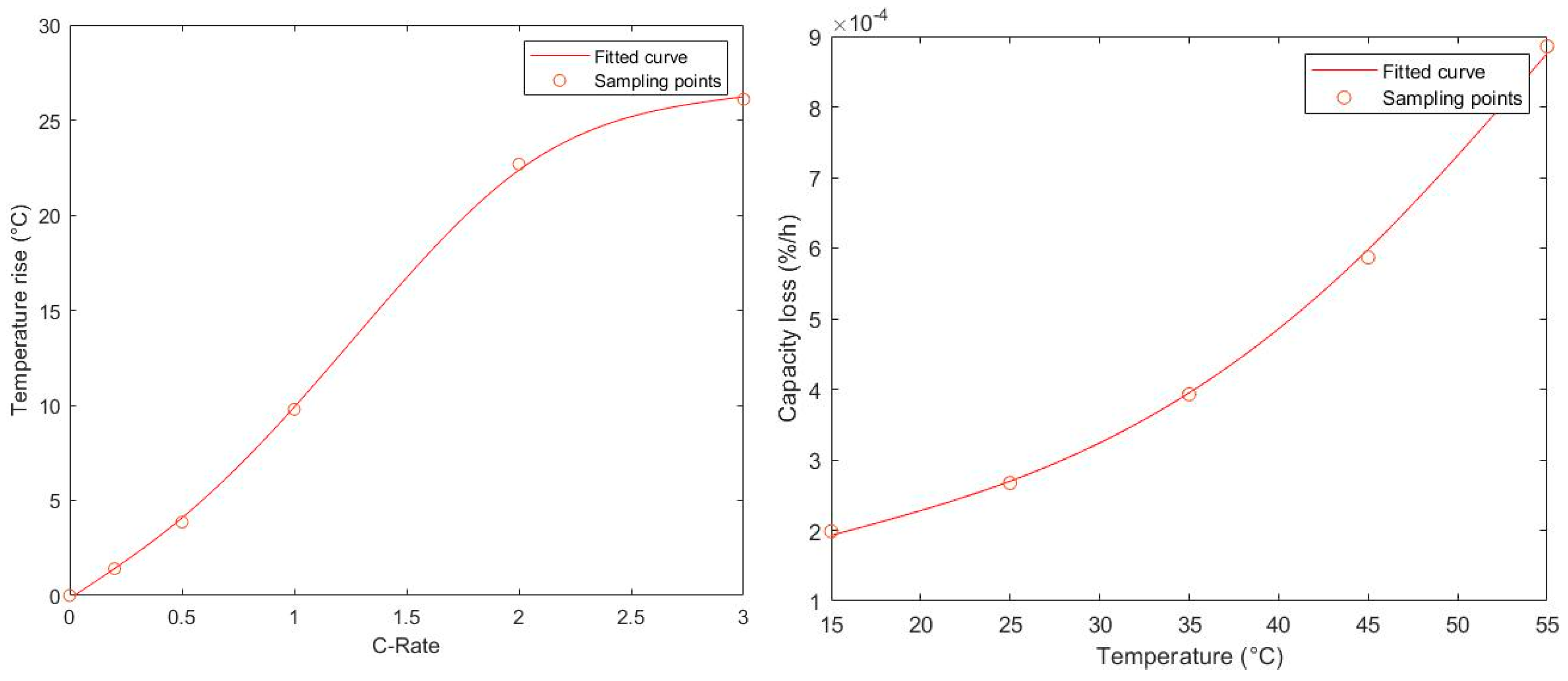
First, the battery temperature, as a dynamic variable during operation, has to be calculated within the model. As the temperature model provided by Simulink as part of the “battery” block cannot be used, because the block is not applicable when using the “phasor” mode, a new temperature calculation path has to be calculated. In the literature, many temperature models have been introduced, but with highly complex calculations based on many parameters to be calculated experimentally, or which are only given for certain LIB types or products. Additionally, most models were also based on Simulink blocks which cannot be used in the designated simulation mode. As this approach aims for a preferably general application, it has been decided that these models are not suitable. This has resulted in the development of our own more general temperature model with a focus on estimation of the temperature by some key factors. The approach presented here is based on the notion that the battery temperature is mainly affected by the C-Rate at which the battery is charged or discharged. Therefore, a study from [
37], where the temperature rise of an LIB in dependency to different C-Rates has been determined, was used. When calculating the average temperature rise inside a cell by using these data, we achieve the temperature rise function shown in
Figure 9.
As the C-Rates of the battery within this approach are very small, thereby resulting in a marginal temperature increase, this approach is fairly appropriate.
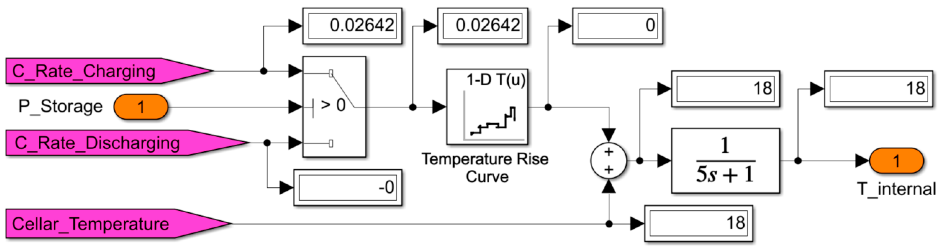
For calculation of the overall LIB temperature, the base temperature of the LIB had to be set. Therefore, it was assumed that the LIB is placed in the cellar. The cellar temperature, which indicates the LIB base temperature, was calculated as follows. First, it is assumed that the cellar temperature does not drop below 18 °C, which was examined by own measurements. Second, the cellar temperature corresponds to the average ambient temperature of the last 7 days, which results in a temperature increase during summertime. The overall internal LIB temperature is calculated as shown in
Figure 10. In the end, for every time step, the capacity loss has to be calculated by usage of the degradation curve shown in
Figure 9 (right). Subsequently, the overall calendar aging is calculated by summing up the capacity losses of every time step.
The calendar aging is given in capacity loss (20% until EoL), while the cycle aging is given in degradation (100% until EoL). Therefore, the capacity loss has been converted to 100% by assuming that a 20% capacity loss means a degradation of 100%. So, both types of aging can be added in the end to achieve the overall aging during one year of simulation. The Simulink model uses a step size where every step characterizes 1 min. So, the “Transfer Fcn” Block in
Figure 10 delays the temperature rise or fall by 5 min.
2.4.2. Lifetime Prediction Model—Fuel Cell
The degradation of FCs is influenced by four main factors [
17]:
Degradation through normal operation
Degradation through starts and stops
Degradation through open circuit
Degradation through fast current changes
The first two factors are of particular importance. It is economically ineffective to run the FC permanently with grid feed-in in case of excess electrical energy in connection with an already full LIB. This results in a more frequently occurring switch-off and switch-on when used in a private household which depends on the SOC of the LIB. Initially, the FC covers the household energy demand via direct usage, while the excess electricity is used for charging the LIB. When the LIB reaches predefined SoCs, the FC power is restricted (see
Section 2.3). This control procedure results in reduced switch-off and switch-on, as shown in
Section 3.2, which guarantees a longer lifetime. The starts and stops of the FC are given by counting how often the control mode “fuel cell operation” has been activated by the energy management system. As not only the switch-on influences the degradation but also the switch-off, the “fuel cell operation” mode activations have been taken twice [
17]. Every start-stop shall influence the degradation by a factor of 14 µV [
39]. The overall amount of starts and stops is multiplied by this factor to achieve the overall degradation through starts and stops.
Fast current changes will also impact the lifetime of FCs, but because of the stationary application in connection with an LIB, fast current changes do not occur often, in contrast to FC cars, for example. The FC power adjustment is controlled to be adjusted smoothly, and changes can occur only once every 15 min. Additionally, the data situation for the degradation caused by fast current changes is insufficient.
As defined in
Section 2.3, the FC is switched off when an SoC of 70% is reached. The FC could also switch into open circuit instead, but with a favourable high storage capacity of the LIB as discussed in
Section 3.5, the LIB can cover the energy demand of the household for a relatively long time of approximately 1 to 2 days. This results in a more beneficial switch-off instead of open circuit operation, wherefore the degradation through open circuit has been neglected. Additionally, the FC power adjustment leads to a less frequently occurring switch-off but longer operation time.
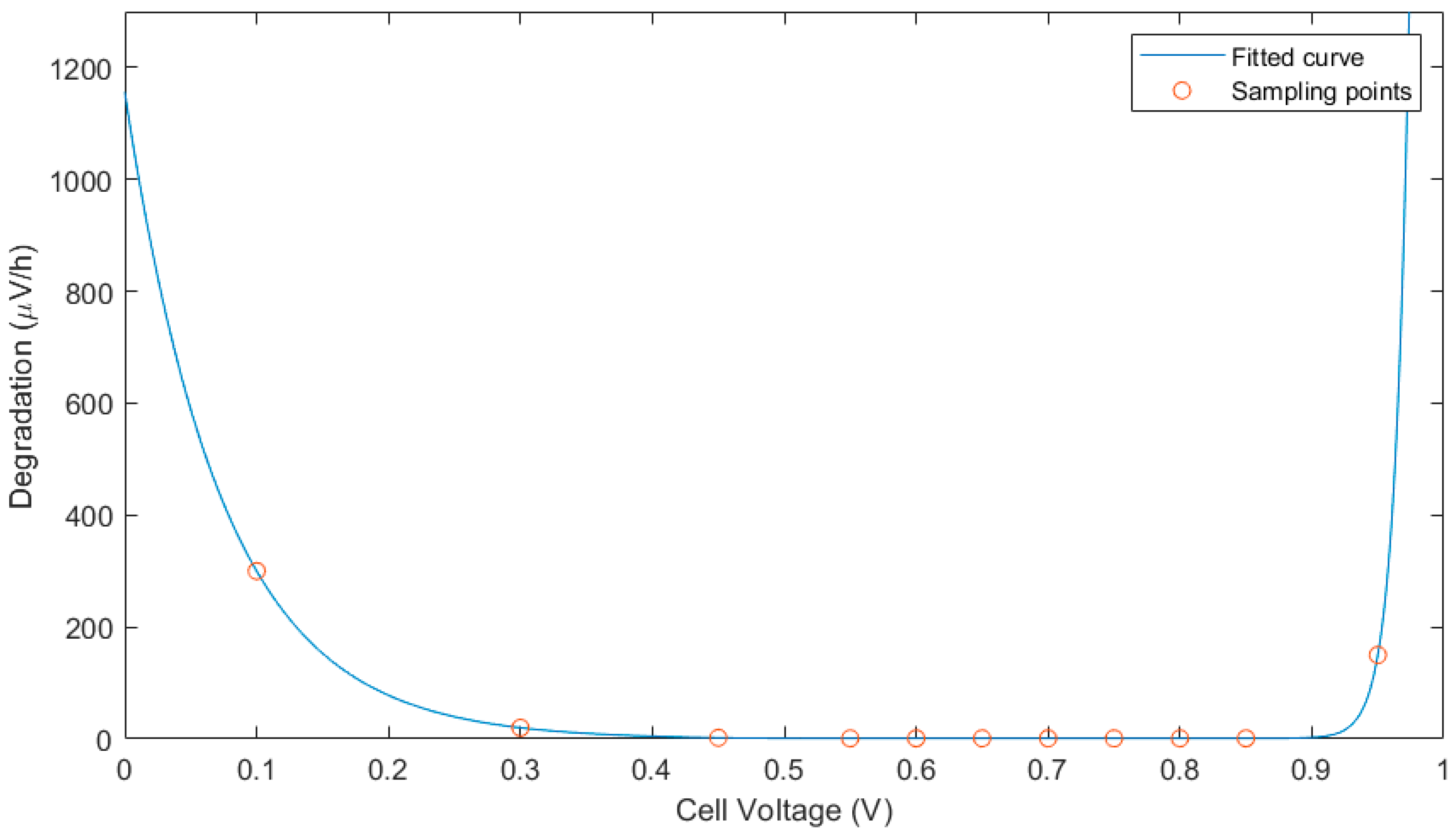
The sampling points describing the degradation of the FC at different cell voltages established from Ms. Bonitz [
17] have been used in this approach. As shown in
Figure 11, the degradation is at a constant low level for cell voltages between approximately 0.2 V and 0.85 V. Instead of using the degradation function established from Ms. Bonitz, a new function which better fits the sampling points was designed but using the same procedure. Therefore, the “fit”-Function from Matlab was used and the function was divided into three value ranges.
Figure 12 shows the functions and coefficients for every value range. These functions result in the degradation diagram shown in
Figure 11. The sampling points summarized in
Table 1 are integrated into the diagram for verification of the function.
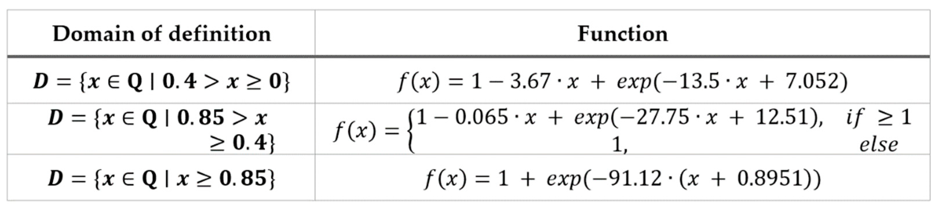
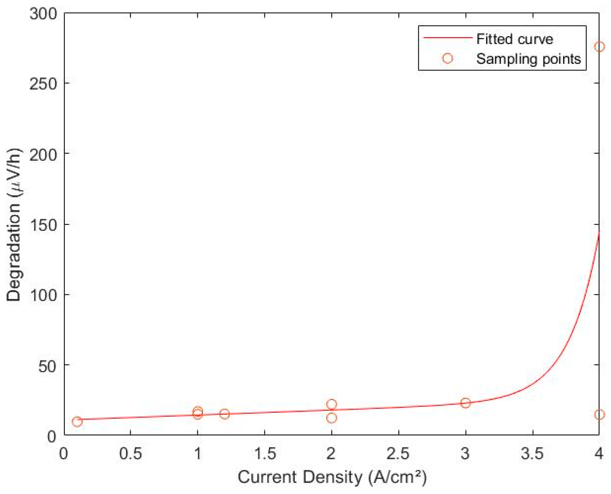
2.4.3. Lifetime Prediction Model—Electrolyser
The next part is the degradation of ELYs. In this area, the research state is still bland. Ref. [
40] says that the impact of volatile loads on the service life of the ELY and its components has been researched very little so far. However, what is similar in every paper that pays attention to the lifetime of ELYs is the fact that degradation is influenced by the current density of the ELY. A paper describing an extensive study of the degradation behaviour of ELYs by different operation modes has not been found in the literature. Instead, some papers have been found where specific degradation behaviours at some key current densities have been proven, which are summarized in
Table 2. For low current densities with up to 3 A/cm
2, the degradation was detected to be approximately linear. On the basis of these sampling points from
Table 2, a degradation function for the ELY was set up using the same principle as Ms. Bonitz for the FC. The literature does not give quantitatively usable insights for other factors influencing ELY degradation. The degradation function established from the sampling points is shown in
Figure 13. The function which describes this trend, which has been calculated by using the fit function from Matlab, is as follows:
2.5. Methodology of the Simulated Lifetime Prediction
Section 2.4.1,
Section 2.4.2 and
Section 2.4.3 gave an overview of lifetime prediction procedures of the three main components, ELY, FC and LIB. These components heavily impact the lifetime of the overall energy system. The lifetime expectation of the PV system is already very high compared to the other components and can reach at least 25 years [
44]. The PV system’s lifetime is mainly influenced by outdoor weather conditions and is therefore hard to evaluate with a simulation. Therefore, the lifetime of the PV system has been neglected within this approach.
As part of the literature research, great importance was attached to the ability to assess and generate the influencing parameters using a simulation. After the end of the Simulink simulation, these data were transferred to Matlab in the form of data series, where the data are first processed and converted into a resolution of one minute. Then, the degradation is read out in the degradation curves depending on the parameter value of the influencing factor (current density, cell voltage, etc.) present in the respective time step. This value is then weighted according to the 1 min resolution, since the degradation is given in µV/h. In this way, the absolute degradation is calculated for each time step and summed up at the end to obtain the absolute annual degradation. In the last step, the life expectancy (in years) was determined based on the common End of Life (EoL) expectancy given in the literature for the respective component, assuming that the course of the year remained the same as given with the used input data sets. Summarizing the previous section, all influencing parameters transferred to Matlab are listed in
Table 3.
3. Results
For the evaluation and the analysis of the lifetime prediction model, some parameter studies were performed. Therefore, different component configurations were compared for single components by leaving the other components at a predefined base configuration. A 720 W FC, a 6.83
PV system, a 20 kWh LIB and an ELY with a nominal output of 5 kW were always assumed as the base configuration. For the PV system, it was assumed that there was no shading all year round. A summary of the main system characteristics assumed in this work is shown in
Table 4.
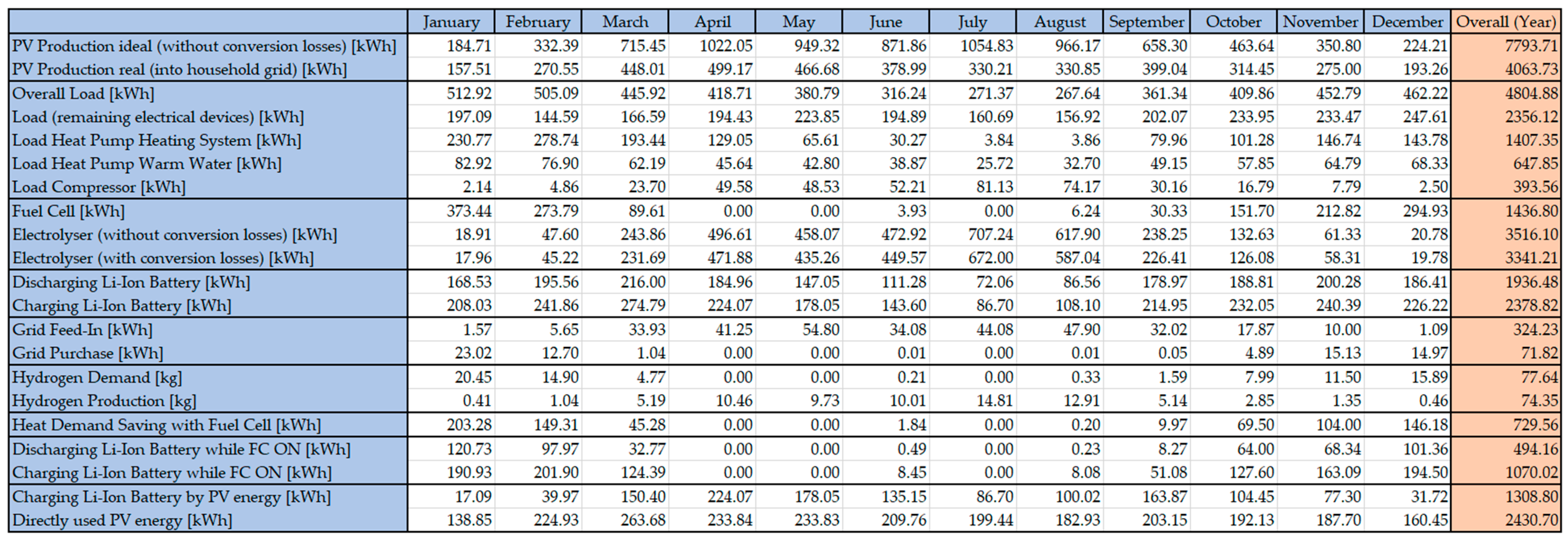
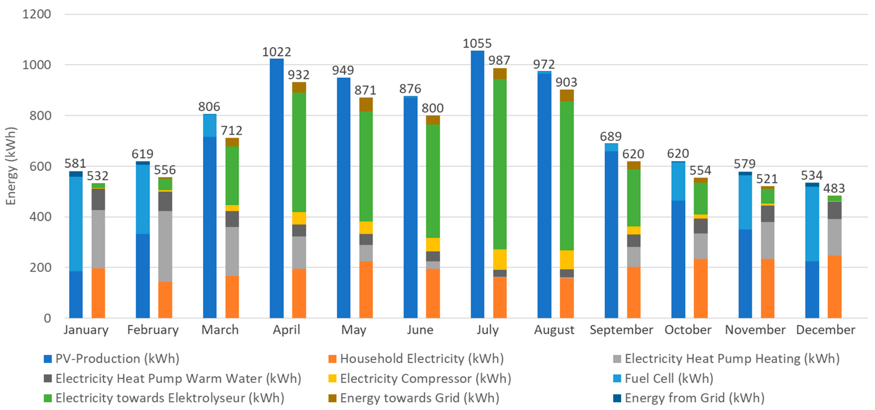
For a better understanding of the energy balance within this paper, the monthly outcomes of the component energy productions and requirements for the base use case are shown in
Figure 14.
Figure 15 shows the monthly production of energy (left bar) compared to the monthly energy demand (right bar). From October to March, the energy produced by the FC is relatively high, while the energy required in these months is higher than during the summer because of the higher heating demand. The green bar shows the surplus energy which is used in the ELY to produce hydrogen.
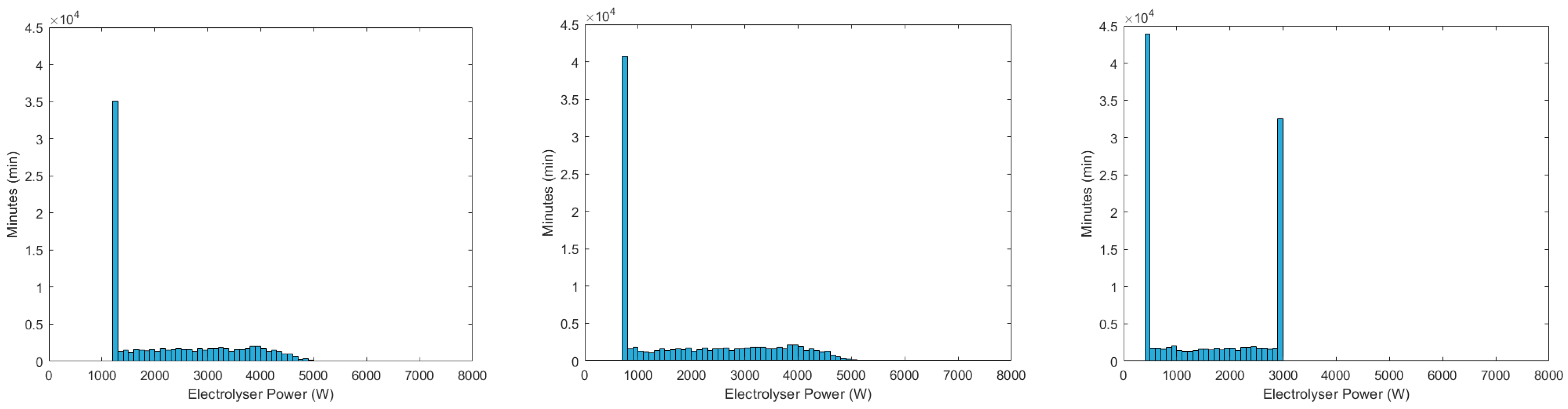
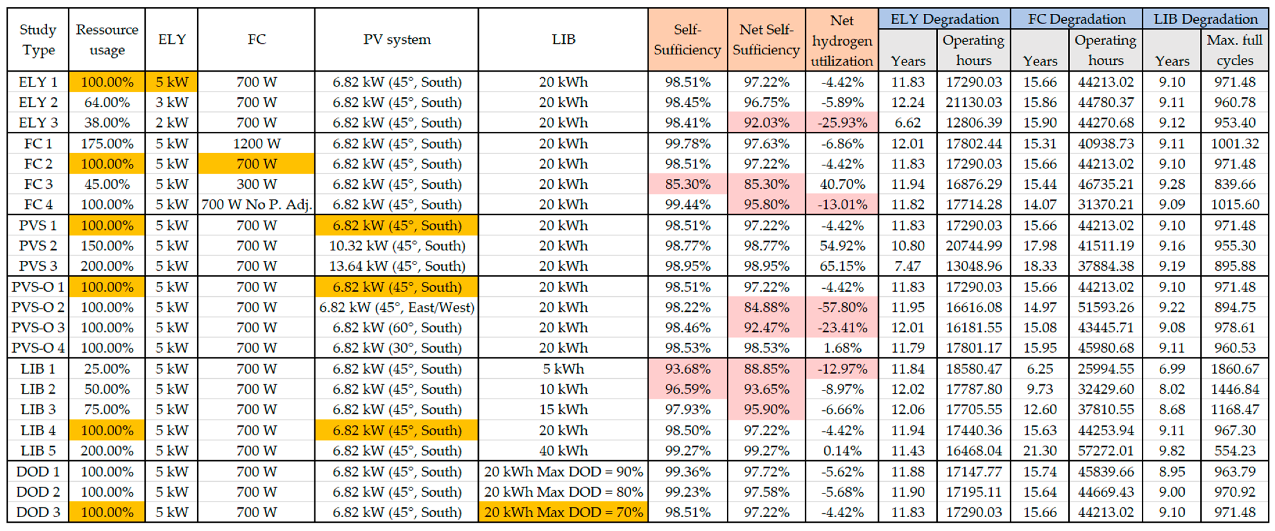
3.1. Parameter Study to ELY Sizing
One part of the parametric study included the impact of different ELY sizes on component life. Three different power classes were compared: 5 kW (ELY 1), 3.5 kW (ELY 2) and 2 kW (ELY 3) nominal power. With acceptance of losses in efficiency, the ELYs can operate at maximum powers of 7.83 kW, 5.01 kW and 2.98 kW, while the minimum power is 1.2 kW, 0.77 kW and 0.46 kW, respectively. As a power of 6.8
under standard test conditions was assumed for the photovoltaic system, the ELY 1 is slightly oversized. The control was designed in such a way that the ELY only switches on as soon as there is a surplus of PV energy which is higher than the minimum power of the ELY, and if the LIB is charged to at least 70% (see
Section 2.3). The ELY initially runs at minimum power until the LIB has reached the maximum charge level. After that, the entire excess energy goes to the ELY, provided that it does not exceed the maximum power. Any energy that exceeds the maximum output is fed into the grid.
The simulation showed deviations in the average efficiency of 70.73% for ELY 1, 68.51% for ELY 2 and 66.09% for ELY 3. The reasons for this are differences in the operating point. While ELY 1 mainly operates at low power, where ELYs are more efficient and have a lower degradation, ELY 3 is more heavily loaded and often even operates at maximum power (see
Figure 16). At the same time, the greater utilization leads to greater degradation as shown in
Figure 17.
While ELY 3 is more heavily loaded, it also experiences greater degradation, which results in a lower life expectancy. The operating hours are also significantly reduced. The results of the lifetime analysis of various ELY sizes are listed in
Figure 17. The simulation showed that the ELY with a nominal output of 2 kW had only a slightly lower hydrogen production within the year. A total of 60.78 kg of hydrogen was produced, compared to 72.32 kg for the 3.5 kW ELY and 74.35 kg for the 5 kW ELY, which is a difference of 15.94% and 18.20%, respectively. If this is compared with the difference in nominal power of 42.86% for the 3.5 kW ELY and 60% for the 5 kW ELY, the difference in the amount of hydrogen production is rather small. However, the 2 kW ELY was often operated at the maximum power limit, which resulted in significantly higher degradation. In this case, the life expectancy fell by 59.9% compared to the 3.5 kW ELY. This shows that an undersized ELY that runs at full capacity does not make sense in terms of life expectancy.
On the other hand, the use of an ELY, which is also designed for the use of occasionally high excess energy from PV, proved to be ineffective. What is meant is the use of the 5 kW ELY instead of the 3.5 kW ELY. In terms of life expectancy, the 3.5 kW ELY performed slightly better: 11.8 years (5 kW ELY) to 12.2 years (3.5 kW ELY). With the 5 kW ELY, only 1.75 kg more hydrogen was produced. The histograms in
Figure 16 show the power distributions of the three ELYs. With the 5 kW ELY, it even had to be fed into the power grid more frequently, which is due to the higher required minimum power. With the 5 kW ELY, 324.23 kWh were fed in, while with the 3.5 kW ELY, only 245.97 kWh had to be fed in.
3.2. Parameter Study to FC Sizing
In the second part of the parameter study, the effects of different FC power on the service life and the energy balance were examined. The input data used in this study resulted in an average electrical output of approx. 700 W in the winter months, considering the household electricity requirement and the electrical energy for hot water and space heating. For the parameter study, three FC sizes were compared, an undersized FC with 300 W (FC 1), a 720 W FC (FC 2) and an oversized FC with 1200 W nominal power (FC 3). The results of the comparison are shown in
Figure 17. The results showed that the 1200 W FC had the highest efficiency due to the lowest average utilization and the lowest operating hours, although the differences were not deemed as being significant. The undersized FC showed the fastest aging with 12.0 years, while the 720 W FC with 15.7 years was even higher than the 1200 W FC (15.3 years). In the study, the 720 W FC had an 8% higher maximum number of operating hours before EoL compared to the 1200 W FC.
When using the undersized FC, 731.18 kWh had to be covered by the grid mainly in the winter months, while with the 720 W FC, only 71.82 kWh was demanded, and with the 1200 W FC, only 10.52 kWh had to be covered by grid. When an energy self-sufficient household is targeted, an oversized FC should be used. However, oversizing the FC led to a lower life expectancy than an FC tailored to the application and the average output, since the oversizing resulted in the FC being switched on and off more frequently. While the FC designed for 720 W had an estimated life expectancy of 15.66 years, the lifespan of the 1200 W FC was 15.31 years. The 1200 W FC was turned on 66 times during the simulated year because it charged the LIB faster and the FC had to be turned off again as a result. In contrast, the 720 W FC was switched on 57 times and the 300 W FC 52 times. These switching on and off processes significantly accelerate aging as described in
Section 2.4.2. It is therefore advisable to dimension the FC as precisely as possible for the application.
Finally, a simulation was carried out in which the 720 W FC was operated constantly at nominal power without power adjustment during operation. This test resulted in almost twice as many starts and stops (96 times), and as a result, led to a reduced life expectancy of 14.07 years. The efficiency was also lower at 45% compared to 48.33% for power-adapted operation, since efficiency decreased with higher utilization. This test showed that FC performance adapted to the state of charge of the LIB had a beneficial effect and is therefore recommended.
3.3. Parameter Study to PV System Sizing
In another study, the effects of different PV system dimensions on the life expectancy of the main components were analyzed. For this purpose, three PV system sizes were compared: 6.82 (PVS 1), 10.23 (PVS 2) and 13.64 (PVS 3). The modules were oriented towards the south with an elevation angle of 45°. The tests showed that an increase in the PV system output had a major impact on the service life of the FC. The simulations were performed using the 5 kW ELY and the 720 W FC. Over the course of a year, the PVS 1 had 77.64 kg of hydrogen, the PVS 2 had 62.02 kg and the PVS 3 had 52.48 kg of hydrogen to be used within the FC for securing energy demand, while 74.35 kg (PVS 1), 137.59 kg (PVS 2) and 150.59 kg (PVS 3) of hydrogen were generated. The comparatively small increase in hydrogen production between PVS 2 and PVS 3 could be explained by the undersized ELY when using the PVS 3. In return, the PVS 3 fed 2483.26 kWh of energy into the grid, while the PVS 2 fed in only 237.09 kWh. Due to the higher utilization of the ELY with increasing PV system size, the life expectancy of the ELY dropped significantly. The service life of the PVS 1 was 11.94 years with 17,440 operating hours; the PVS 2 had a service life of 10.8 years (20,745 h), and for PVS 3, it was 7.47 years (13,049 h). Two effects occurred with the FC: The service life of the FC increased with increasing PV system size (15.66 years (PVS 1), 17.98 years (PVS 2), 18.33 years (PVS 3)), but the maximum operating hours decreased due to more frequent starts and stops (44,213 h (PVS 1), 41,511 h (PVS 2), 37,884 h (PVS 3)).
However, the PVS size did not have a significant effect on the LIB life expectancy. In each case, the lifetime until EoL and the maximum full cycles during the period were almost identical.
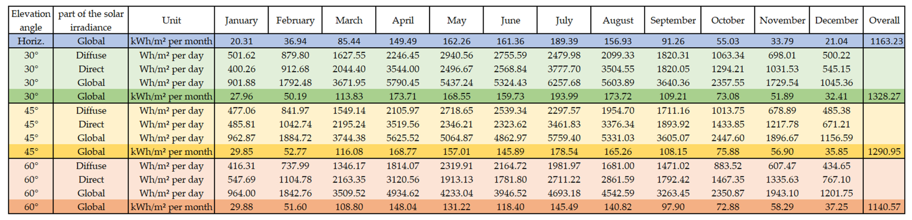
3.4. Parameter Study to PV System Orientations
The impact of different PV system orientations and elevation angles has also been studied. The following orientations have been compared: A standard orientation towards the south (azimuth angle
) with an elevation angle of
(PVS-O 1), an east- and west-oriented PV system with
(PVS-O 2), an orientation towards the south again but with
(PVS-O 3), and last, an orientation towards the south with
(PVS-O 4). The DWD provides global and diffuse irradiation profiles measured for a horizontal plane only. Due to this, the irradiation profile for an inclined plane had to be calculated first using the formulas described by Quaschning [
45]. The monthly energy yield for the horizontal plane and for all three elevation angles separated into diffuse and direct parts are shown in
Figure 18. The positioning of the PV system was assumed as ideally having no shadowing during the whole year. To generate realistic data, losses due to pollution, conduction losses, etc., have been considered by introducing an efficiency parameter, which was set to 90%.
In each case, the same overall number of modules (22 modules à 310
) have been used. The different orientation did not have a significant influence on the ELY and LIB lifetime. The FC lifetime was highest at PVS-O 4 (15.95 years) and lowest at PVS-O 2 (14.97 years). Of greater importance was the impact on the net hydrogen utilization (see
Figure 17), which tells how much hydrogen has been produced compared to the amount of hydrogen required for the FC. If the net hydrogen utilization is negative, more hydrogen was required than was produced. PVS-O 2 resulted in a large hydrogen deficit of −57.8%, which was caused by less energy production from the PV system. Moreover, PVS-O 3 caused a hydrogen deficit of −23.4%, although this elevation of 60° is better for energy production during wintertime in Germany. Using PVS-O 1, the PV system produced 7794 kWh energy, PVS-O 2 produced 6348 kWh, PVS-O 3 produced 7198 kWh and PVS-O 4 produced 8013 kWh. The study showed that an energy production shift towards wintertime is not meaningful, and that an east and west orientation is also not meaningful.
3.5. Parameter Study to LIB Storage Capacities
Next, different LIB storage capacities were compared: 5 kWh (LIB 1), 10 kWh (LIB 2), 15 kWh (LIB 3), 20 kWh (LIB 4) and 40 kWh (LIB 5). LIB 1 aged 1 year faster (7 years) compared to LIB 2, which was twice the size (8 years), and again aged 1 year faster than LIB 4, which was four times larger (9 years). LIB 5 had the longest lifetime with 9.8 years. However, the utilization of LIB 1 with 1861 full cycles until EoL was significantly higher than that of LIB 5 (554 full cycles).
The LIB storage capacity had a significant impact on the FC, which was due to higher utilization on the one hand, since more energy had to be provided via the FC with less energy storage capacity, and on the other hand, to the more frequent starts and stops (LIB 1 was fully charged faster than LIB 5).
The service life of the FC when using LIB 1 was 6.25 years (26,000 operating hours), with LIB 2 it was 9.7 years (32,430 operating hours), with LIB 3 12.6 years (37,810 operating hours), with LIB 4 at 15.7 years (44,213 operating hours) and with LIB 5 even 21.3 years (57,272 operating hours). On the other hand, the LIB storage capacity had hardly any influence on the service life of the ELY. The lifespan only varied between 12.1 and 11.4 years.
3.6. Parameter Study to LIB Max. DoDs
The influence of different maximum DoDs on the lifetime was also investigated using the 20 kWh LIB storage capacity as a reference. A maximum DoD of 90% (DoD 1), 80% (DoD 2) and 70% (DoD 3) was examined. The number of full cycles for all three variants remained almost identical at around 107.1. The variation of the maximum DoDs had little influence on the life expectancy. The life expectancy at 90% max DoD was 8.95 years, at 80% max DoD, it was 9.00 years, and at 70% max DoD, it was 9.10 years. This is because in this stationary application case, cyclic aging does not have a significant impact, since 107 full cycles within one year are comparatively few compared to the full cycles up to EoL of 6000 to 10,000 that are theoretically possible today. Even the 5 kWh LIB only had 266 full cycles during one year.
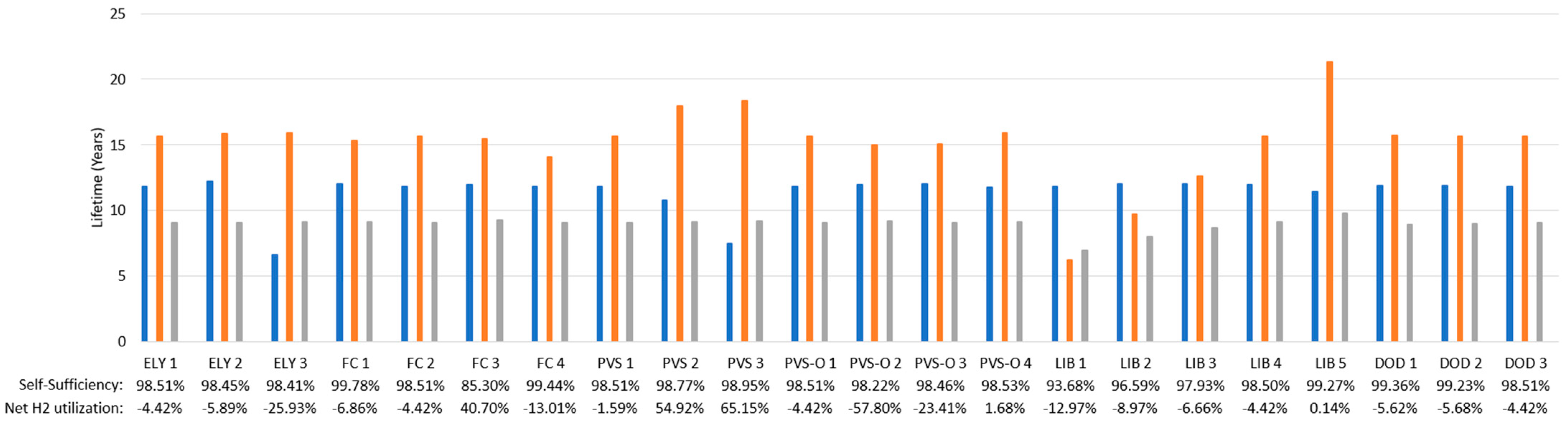
Figure 19 shows a graphical comparison in terms of lifetime for all parameter studies.
4. Discussion
The simulation based on the Simulink model allows a detailed and meaningful analysis of hydrogen-based energy systems especially because of the high resolution of the input data. Due to the usually strong fluctuating load, temperature and irradiation profiles, a simulation with a resolution of 15 min allows a more precise statement about the suitability and sizing of various components compared to analysis procedures with monthly or daily averaged datasets. This resolution also allows an evaluation of the lifetime expectations of the main components which on the one hand is related to the control algorithm. As Simulink allows a detailed design of such a control system, a meaningful impact analysis can be performed.
A negative net hydrogen utilization from some of the parameter studies (see
Figure 17) can be compensated by an increase in the PV system dimensioning mostly. But for achieving a high self-sufficiency the FC and LIB configurations and control are most important and should be adjusted in dependency to the designated use case. Inappropriate PV system orientations have a high impact on the net hydrogen utilization (see
Section 3.4). A better orientation for the summer month for reaching higher overall energy yield is more meaningful at least for Germany but it depends on the designated use case (see
Figure 18). As shown in
Figure 18, a PV system with an elevation angle of 60°, which, especially for Germany, should be better for winter month compared to an elevation of 45°, reaches nearly the same energy yield in January due to the high diffuse solar irradiance portion. In return, however, the energy yield in the summer months is significantly lower at an elevation angle of 60° compared to 45°.
The energy system depends on the climatic conditions with regard to the installation site. On the one hand, limiting temperatures for the operation of the components play a role, and on the other hand, the climatically determined energy demand and generation, which influence the profitability of the system. In this paper, the system was designed for use in the temperate climate zone and Würzburg (Germany) was assumed as the location with an average horizontal solar energy yield of 1170 kWh/m2 measured between 2001 and 2020. A suitable dimensioning for different climate conditions can be found using the model presented here by arbitrarily adjusting the input data. The hydrogen-based energy system is especially useful in regions where the energy production from renewable sources is not sufficient to cover the year-round energy demand by usage of short-term energy storage due to significant seasonal changes. The use in the form of a self-sufficient energy system for a private household is also limited by the available area for the installation of PV modules. FCs and ELYs can be scaled based on the number of cells.
In the parameter study, the life expectancy of the ELY is 11.4 years in average (with approx. 17,250 operating hours), the FC reached a lifetime of approx. 15.19 years in average (42,629 operating hours) and the LIB reached 8.98 years in average (1011 full cycles). The number of operating hours that are theoretically possible, based on state-of-the-art technology, are about 40,000 h for the PEM ELY [
46], 12 to 15 years for the FC with maximum operating hours of 40,000 to 80,000 h [
47], and lifetimes of about 5 years with over 2000 cycles are common for the LIB [
48].
The lifetime of ELYs is strongly dependent on the operating conditions and deviate significantly from the test-bench specifications given by the manufacturers in real world applications. The lifetime data from literature can also be achieved by using the model presented here, provided that idealized operating conditions have been assumed, for example, for low utilization and continuous operation of the ELY. As research on ELYs specifically designed for the production of green hydrogen has gained momentum in recent years, strong advances have also been made in lifetime the past years. In view of this, it makes sense to adjust the underlying degradation values to the current state-of-the-art at the time the simulation is performed.
The average FC operating hours determined from the simulation are within the range reported by the literature. However, the given maximum number of operating hours (of up to 80,000 h given in literature) are mostly based on studies carried out in continuous operation and can therefore hardly be achieved in real application scenarios as presented in this work. If the FC would not have required such a high number of starts and stops in the application scenarios, significantly more operating hours would have been possible.
Due to the lower number of full cycles of the LIB in all parameter studies of about 1011 full cycles in average until EoL, it is realistic that the manufacturer’s specifications for life expectancy of 5 years [
48] will be exceeded, proportional to the simulation carried out. It was shown, that calendric aging has a decisive influence on the EoL.
The simulation was performed using a 15 min time resolution since otherwise the simulation effort would have been extremely time consuming, whereby the input dataset for the load had to be averaged, and, as a result, sudden rapid changes in the dataset have been neglected. Component ramp-up and start-up times have not been considered, while they are neglectable in the considered time scale. A higher resolution of the entire input data failed due to the weather and solar irradiance datasets that were only available in hourly resolution. Therefore, input datasets with a much higher resolution which we are actually recording by our own will be involved in future research. This may also have an impact on the lifetime expectations of the components.
5. Conclusions
This work presented a methodology to simulate the lifetime performance of hybrid hydrogen-based energy systems for private households designed for high self-sufficiency levels. A literature review on the lifetime behaviour of the three main components, ELY, FC and LIB was carried out; the extracted data were prepared for the application in a Simulink model under variable operation conditions of the components. This Simulink model has been validated in a previous publication [
3], and it was used to design a household power system based on real data covering an entire year in 15 min resolution.
The energy management system used in the model was also presented; it was designed with the aim to maximize component lifetime and efficient use of energy.
As part of the work, a parameter study was carried out. Based on this, an evaluation of the energy balance, the hydrogen demand, and the lifetime of the main components was performed for various dimensionings: It showed that the components are highly interdependent on each other and should therefore be precisely dovetailed together in advance before system implementation. The energy demand, energy utilization behaviour, and the desired degree of self-sufficiency must also be considered in the layout.
Within the parameter study, the change of lifetime expectations when changing the component dimensionings is shown. In addition, the variation of a component not only touches its intrinsic component lifetime, but also has an effect on the other components. The lifetime of the FC could be significantly increased by increasing LIB storage capacity, which is mainly caused by the less frequent switch-on and switch-off processes of the FC when recharging the LIB. However, as the storage capacity increases, the utilization rate of the LIB (expressed in the full storage cycles) decreases. Although this also increased the lifetime of the LIB, the usual maximum full cycles were not even reached until EoL, since the use-independent calendric aging process of the LIB became the decisive criterion for aging here. In terms of the cost performance, a smaller LIB performs better in this case. The next step will be to conduct an economic analysis to draw conclusions about the capital employed for the overall system and thus better assess the usefulness of increasing the capacity of the LIB to increase the lifetime of the FC. The size of the LIB also has a significant impact on hydrogen utilization, as shown in
Figure 17. By increasing the total capacity from 5 kWh to 40 kWh, the net hydrogen utilization was brought from a deficit of −12.97% to + 0.14%. This is primarily due to the increased efficiency from the increased short-term storage by the LIB, which decreases the gross energy demand.
An increase in PV system size also led to an increase in FC lifetime. In addition, a power-adjusted control of the FC also makes sense with regard to the FC lifetime and the degree of self-sufficiency.


