Life History Strategy of Maurolicus muelleri (Gmenlin, 1789) in the Bay of Biscay

Abstract

Maurolicus muelleri is a significant component of the marine ecosystem and has the potential to be a valuable fishery resource. However, in the Bay of Biscay, its primary biological traits remain unclear. This study presents data on the length distribution, age, growth, maturity ogive, spawning season, batch fecundity, and sex ratio for Maurolicus muelleri captured in the Bay of Biscay. The results showed that in spring, the adult spawners (ages of 1 and 2) were dominant in the catches, while in September, immature juveniles (age of 0) born in spring were mostly found. Using standard lengths as a basis, 50% of the fish were mature at 34.1 mm (both sexes combined), and the sex ratio, male to female, was 0.44:0.56. The proportion of females increased with length, and a 1:1 sex ratio was predicted at a standard length of 41.5 mm. The spawning season was allocated to at least between March and September, with a likely peak in May. The batch fecundity ranged from 114 to 919 oocytes/female, and increased with the weight and length of females. The results allowed us to interpret a life history strategy for this species, i.e., a high fecundity for females, which mostly participate in one or two reproductive seasons. Therefore, any possible exploitation of age 0 fish prior to spawning could lead to a decrease in the population from which recovery could be slow.

1. Introduction

Mesopelagic refers to the twilight zone of the water masses [1], where surface light is still detectable in the daytime, but at very low levels compared with the epipelagic zone. This zone is usually considered to extend from about 200 to 1000 m in depth [2,3]. Many of the inhabitants of this zone carry out diel vertical migrations (DVMs) [2], residing at lower depths during the day and swimming towards the surface to feed at shallow depths at night. DVMs are recognized today as the biggest movement of biomass on Earth [4], with major consequences for ecology [1] and biogeochemical cycling [5]. Additionally, the high biomass and shoaling behaviour imply a potential for fishing in some areas [6,7], and these organisms serve as an important prey source for many predatory fishes [8].

One of the most common species inhabiting the mesopelagic ecosystem is the pearlside, Maurolicus muelleri (Gmelin). M. muelleri occurs in a high abundance near continental slopes in the southeast Pacific [6,9], the northwest Pacific near Japan [8], the South Atlantic [10,11], and the northeast Atlantic [12]. Although the mesopelagic family is principally oceanic, M. muelleri seems to be associated with land masses, spending daylight hours near the bottom at depths from 100 to 500 m and rising into shallow water in large shoals at night where it apparently feeds [8,9,13]. Continuous acoustic observations of pearlside sound scattering layers (SSLs) revealed that adult fish, which constitute the deepest SSLs, did not engage in DVMs between late autumn and early spring, whereas younger life stages, forming shallower SSLs, displayed DVMs during the same period [14,15]. DVMs seem to be related to an improvement in feeding conditions [16] and/or reduced predation risk. Previous studies suggest that pearlsides feed visually during daylight hours and that their foraging depth and diet composition may vary seasonally [17,18].

The abundance and biomass of mesopelagic fishes are currently involved in a controversial debate. The most recent estimations of the mesopelagic fish biomass by combining acoustic and ecosystem models have reduced the previous acoustic-based estimation values of 11–15 billion tonnes [19] to about 2 billion tonnes [20]. These high biomass estimates sparked interest in the potential exploitation of mesopelagic species to produce fish meat, fish oil, and nutraceuticals [21,22]. In the northeast Atlantic, a trial of the commercial exploitation of mesopelagic resources has not been very successful [23,24] due to low catch levels. This could be associated with temporal changes in the spatial migration patterns of these species [22], which would have limited their availability in the fishing area. The impact of commercial trawling on the mesopelagic fish population is uncertain. Despite not being a target species for most fisheries, the presence of mesopelagic fish as a bycatch in some mid-water trawls seems to be common [25,26]; although with the information recorded at present, this does not generate large amounts of bycatch [25]. Given the ecological significance of mesopelagic fish in the marine ecosystem, the potential exploitation of this community should be carefully investigated.

Studies on the biology and vertical distribution of M. muelleri around the world are extensive. In areas such as the Norwegian Fjords, South Pacific, and South Africa, the studies date back to the late seventies. It is known that M. muelleri is a small (4–5 cm), short-lived fish (maximum of 5 years), and only a small proportion of the population reaches the age of 3 years [12]. In other areas, such as the Rockall Trough, the longevity may be closer to 1 year [14]. In general, mesopelagic fish have a slower growth than epipelagic fish [27], but due to their short life cycle, they have higher fecundity rates. Gjøsæter [28] was the first to report fast growth until sexual maturity is reached and then very slow subsequent growth; Goodson et al. [29] remarked on the difference between fish aged 1 year and fish aged 2 + years. The length vs. age relationships yield a high variability in the slope values [18,29,30,31] due to the high dependence of this relationship on the size range and number of samples.

The life history of M. muelleri in the Bay of Biscay is currently not well understood. Some references to the presence of eggs and larvae were reported by Arbault and Boutin [32], Valencia et al. [33], d’Elbée et al. [34], Rodriguez et al. [35], and Rodriguez [36] in the southern Bay of Biscay. An increase in adult abundance that was linked to climate change was published in the Cantabrian Sea by Puzón et al. [37]. The importance of Maurolicus in the diet of albacore tuna was reported by several authors. Ortiz de Zarate [38] observed the presence of M. muelleri in the stomachs of immature albacore tuna. Later, Pusineri et al. [39] found that the diet of albacore tuna consisted mainly of Maurolicus (79%) that were ingested at night when the Maurolicus fish performed their vertical migration.

The goal of this study is to contribute with new biological knowledge about the most relevant demographic parameters of this species, such as the age, sex ratio, length at first maturity, spawning season, and fecundity. These findings are then used to discuss the history life strategy of this species in the Bay of Biscay.

2. Materials and Methods

2.1. Sampling Area and Sample Collection

Most of the data were collected during the JUVENA acoustic survey [40] that took place in September of 2019 and 2020 in the Bay of Biscay (Figure 1,

Table 1. Description of surveys contributing to the collection of M. muelleri samples in the Bay of Biscay. We defined samples as “extra” samples, which are those taken from the AZTI database to complete an analysis, or “ad hoc” samples, which are those collected specifically for this study. The number of samples for each analysis is also mentioned. RM = RV Ramón Margalef, EA = RV Emma Bardan, VE = RV Vizconde de Eza, SL = standard length, TW = total weight, EW = eviscerated weight, GW = gonad weight, and A = age.

Survey	Vessel	Date	Sample Type	Parameters	Analysis	No. Specimens	ST-T50m (°C)
JUVENA 2016	RM, EA	31 August–6 October	extra	SL, maturity	Maturity ogive	212	20.0–15.9
JUVENA 2017		1 September–9 October			Maturity ogive	260	19.6–18
JUVENA 2018		1–30 September			Maturity ogive	309	20.3–15.7
JUVENA 2019	RM, EA	1–30 September	ad hoc	SL, TW, EW, GW, maturity, A	All except fecundity	874	20.0–17.4
JUVENA 2020		1–30 September	ad hoc			500	21.1–17.6
MEGS 2019	RM	1–6 April	extra	SL, TW, EW, GW, maturity, A	All except fecundity	62	12.6
BIOMAN 2020	VE, EA	4–10 May	extra	SL, TW, EW, GW, A	All except fecundity	138	12.7
BIOMAN 2021		4–8 May	extra	SL, TW, GW, fecundity	Fecundity	100	12.6

).

The survey area was covered by two research vessels, the Ramón Margalef and the Emma Bardán, with the former covering the outer area (oceanic waters) and the latter covering the shallower waters of the northern French area. An adaptive sampling scheme was adopted to cover the whole occupation area of anchovies, thus limiting the area of study of M. muelleri to the presence of anchovies. Sampling was carried out by following a regular grid of transects arranged perpendicularly to the coast and spaced at 15 nm [40].

This acoustic survey focused on an annual assessment of the juvenile portion of the anchovy population and covered an area from the coastal waters to offshore areas well beyond the continental shelf.

With the aim of increasing the number of samples to perform some analyses (see Table 1), we used additional samples. On the one hand, the AZTI database provided information on M. muelleri collected during the JUVENA survey in 2016, 2017, and 2018. On the other hand, we collected extra samples from two more campaigns in the area: the international mackerel and horse mackerel egg survey (MEGS) in the spring of 2019 [41], and BIOMAN in the spring of 2020 and 2021 [42]. Table 1 provides more details.

In all these surveys, M. muelleri were caught using a pelagic trawl net with a 4–10 mm mesh size and mouth openings of 12 ∗ 25 m. For each positive haul, three sub-samples of M. muelleri were retained and conserved in different preservatives according to the subsequent use: in 4% formaldehyde for histological procedures, and at −20 °C for morphometric studies and age determination. Additional data such as the position of capture, date and time, sampler and bottom depth, temperature, salinity, and dissolved oxide (if available) were also recorded.

2.2. Laboratory Procedures

Mesopelagic species were initially identified according to the morphological characteristics of the fish, mainly by the number and position of the photophores. In some cases, when the general condition of the samples made the identification of the species difficult, it was necessary to complement the analysis with additional characteristics for the identification, such as the otolith form [43].

The total length, standard length, total weight, eviscerated weight (weight of fish without gonads, digestive tract, liver, and heart), and both the stomach and gonad weight were measured for each individual, and the otoliths were extracted. Additionally, the sex was determined by a macroscopic analysis of the gonads. When possible, the sexual maturity status was also assigned according to a six-key scale [44]: (1) immature, (2) early ripening (developing, but functionally immature), (3) late ripening and/or early partially spent (developing, but functionally mature), (4) ripe (actively spawning), (5) late partly spent (capable of spawning), and (6) spent (regressing/regenerating).

The annual age of M. muelleri was determined from a reading of the otoliths (sagittae) (see Figure S1). After extraction, the otoliths were washed thoroughly and dried. The observations of entire otoliths were made under reflected light against a black background using dissection microscopes with 20–25× magnification. The process of age determination is a delicate task that is susceptible to many sources of error [45]. For this reason, applying different methods of validation is strongly recommended [46,47]. To age M. muelleri, we used the same criteria as for anchovies, namely the following: (1) An annulus consists of one opaque ring and one hyaline ring. The age equals the number of true complete hyaline rings previously defined. (2) The edge of the otolith is considered hyaline or opaque if this structure is continuous all around the otolith margin. The date of capture is also considered in the aging process. (3) The birth date was set to 1 January. For details, consult the ICES [48]. In addition, the accuracy of the readings was checked by a calibration exercise, where 50 of each year’s otoliths were read independently by two people and reread and discussed if there was disagreement. If no agreement was reached, the otoliths were not used. In this line, it is worth mentioning that some otoliths were also discarded due to complexity in age interpretation. The timing of the formation of the hyaline and opaque zones was defined according to Gjøsæter [12].

To estimate the maturity ogive and the sex ratio, additional samples of M. muelleri collected in previous acoustic surveys during September of 2016, 2017, and 2018 were used (JUVENA 2016/17/18, Table 1).

In those samples kept in a formaldehyde solution, the ovaries were removed and processed in line with standard histological preparation techniques [49]. The lengths and weights for individuals preserved in formaldehyde were corrected for changes due to the preservation using a conversion factor of 1.0194 and 1.0579, respectively [50]. Once the ovaries were removed, the ovary was used for a histological preparation or for an estimation of the batch fecundity. The batch fecundity, defined as the number of oocytes spawned by a female in a single spawning event, was determined by using the gravimetric method on 50 ripe females collected in May of 2020 and 2021, which involved identifying and quantifying the hydrated oocytes in the gonad [51]. The number of hydrated oocytes per gram of ovary-free weight and the whole weight of the female were estimated.

2.3. Data Analysis

2.3.1. Growth Analysis

Standard length and total length: With the aim of estimating a factor to convert standard length (SL) to total length (TL) and vice versa, a simple linear regression was fitted to the fish SL (mm) and TL (mm) data.

$$Y=a+b\times X$$

(1)

where X and Y are the SL (in mm) and TL (in mm) depending on the parameter to be estimated.

Growth in weight with the standard length: To examine the differences in the weight vs. length between years and sexes, a generalized linear model was first used to assess whether the interactions among the parameters of growth, years, and sex were significant. As the sample sizes for sex and year were not sufficient (n < 30 for each sex), the parameters of the length–weight relationship model by sex were calculated using both years together. The model was selected using Akaike’s information criterion (AIC). When significant, pairwise comparisons of slopes were conducted using an ANCOVA model. When the differences between the slopes were significant, the regression model was refitted, excluding the interaction term. When the differences between the slopes were not significant, a new regression model that excluded the interaction term was fitted, and both regression models (with and without the interaction model) were compared using ANCOVA.

Relative condition factor: Two different condition indices were estimated to quantify individual states of health. On the one hand, Fulton’s condition factor index was estimated, which, despite being the most widely used in the literature, is known to depend on several factors (size range, water content, both gonad and stomach weights, etc.) [52,53].

$$Fulton=\frac{EW}{S{L}^3}\times 100000$$

(2)

On the other hand, the Le Cren condition factor [54], Kn, is defined as

$$Kn=\frac{E{W}_0}{E{W}_c}$$

(3)

where EW₀ is the observed weight and EWc is the calculated weight. When Kn ≥ 1, the fish is categorized as being in a good growth condition compared to an average specimen of the same length, while the individual is in poor growth condition when Kn < 1. The total weight and eviscerated weight were used when determining this parameter. By using the eviscerated weight, seasonal differences in the fish condition, derived from the differential contribution of gonad weight and stomach weight to the body weight, were not accounted for.

2.3.2. Maturation Analysis

Gonadosomatic index (GSI): The gonadosomatic index was worked out as the relationship between the gonad weight (GW) and eviscerated weight (EW) as a percentage. Its variation over time indicates the period of greatest reproductive activity. Statistical differences amongst years were assessed using Kruskal–Wallis analyses, and pairwise comparisons of this parameter were performed using Dunn’s multiple comparisons test.

Batch fecundity: A linear model and generalized linear model (GLM) with gamma error distribution were used to assess the influence of the female gonad-free weight and SL (GLM model) on the number of oocytes in the batch.

Maturity ogive: To calculate the probability of “success” for a given fish to reach maturity, logistic regression was selected. The model was fit in R with a GLM binomial distribution. To obtain a minimum number of 10 individuals per size range, the specimens were grouped by 5 mm SL ranges. Since the number of sexed M. muelleri was low, especially for the smallest range distribution, the individuals categorized as immature were duplicated and assigned to male or female. This allowed the distribution of the sizes to be extended towards the smaller ranges.

The standard length at 50% maturity (SL₅₀) was defined as the SL at which 50% of the fish were mature. A GLM with a binomial distribution was used to account for the binary response (mature/immature) and calculate the probability of being mature for each length class.

The parameters of the maturity ogive (SL₅₀ and r, the slope of the curve) were estimated for males and females separately and for both sexes combined.

Sex ratio: A GLM with a binomial distribution was used to assess the proportion of females to males by SL class. The standard length at which the male-to-female proportion reached a value of 1:1 was defined as the SL at which 50% of the fish were female.

Statistical differences in the condition factors amongst years and months were assessed using Mann–Wilcox or Kruskal–Wallis analyses, and pairwise comparisons of this parameter were performed using Dunn’s multiple comparisons test.

All models were fitted using the package MASS in R [55].

3. Results

3.1. Length Frequency Distribution and Body Size Relationships

Individuals collected in pelagic trawls in September of 2019 and 2020 in the Bay of Biscay ranged between 18 and 52 mm for the SL in 2019 (Figure 2, Table S1) and between 18 and 55 mm for the SL in 2020 (Figure 2). Although the length distribution range was similar between years, in 2019, very few individuals had an SL longer than 40 mm. In 2019, only 15 individuals were sexed (ten males and five females), as most of the specimens captured that year were immature, with gonads that were too underdeveloped to assign sex “de visu”. In 2020, the number of individuals with well-developed gonads was higher, and we were able to identify 104 males and 92 females. The minimum and maximum sizes depended on sex. When considering both years, the males ranged from 30 to 55 mm for their SL, whereas females ranged from 37 to 53 mm for their SL. The length frequency distribution of M. muelleri showed statistically significant differences (χ² = 54.21, df = 1, p < 0.001) in the mean size between years. In 2019, the population of M. muelleri was mainly represented by individuals with an SL smaller than 35 mm, with 82% compared to 57% in 2020, while larger individuals (SL ≥ 40 mm) accounted for 12% and 21% in 2019 and 2020, respectively. Several modes were observed in both years, with the most relevant being at 21.6 mm and 23.5 mm, the second at 30.6 and 29.8 mm, and the third at 44.9 and 44.5 mm in 2019 and 2020, respectively.

The length distribution of M. muelleri obtained in additional samples from the MEGS and BIOMAN surveys (see Table 1) varied seasonally (Figure 2). In April of 2019 (62 individuals) and May of 2020 (138 individuals), the most frequent sizes were 42 and 44 mm, respectively. This contrasts sharply with the distribution seen in September, which was composed mostly of individuals smaller than 35 mm. In April and May, only 18 individuals were not sexually identified. The remainder were 57 males, which ranged from 35 to 48 mm for their SL, and 125 females, which ranged from 37 to 53 mm for their SL (Table S1).

The standard length (SL) and total length (TL) presented a strong positive linear relationship between variables (adjusted r² = 0.997). The SL–TL relationship was described by the following equations:

TL = 1.727 (±0.054) + 1.134 (±0.00158) ∗ SL (ANOVA, F = 4.899 ∗ 10⁵, p < 0.001, gl = 1567)

and

SL = −1.418 (±0.049) + 0.8793 (±0.00123) ∗ TL

The strong relationships indicated that, depending on the size of the fish, the caudal fin would represent between 14% and 19% of the total length of the fish.

The total weight and standard length (with both variables log-transformed) had a strong positive linear relationship (r² = 0.97) (Figure 3,

Table 2. Results of the generalized linear model (GLM) testing the influence of year in the relationship between standard length and total weight: logTW = log(SL) ∗ year, with 0 = 2019 and 1 = 2020. *** = 0. (All sexes included.).

Variable	Estimate	S.E.	t-Value	p
(Intercept)	−11.84508	0.06743	−175.658	<2 × 10−16 ***
Log(SL)	3.13318	0.01981	158.196	<2 × 10−16 ***
Year	0.40785	0.09519	4.285	1.96 × 10−05 ***
Log(SL):Year	−0.10373	0.02764	−3.753	1.82 × 10−04 ***
gl residual: 1370; AIC: −1724.4. Model significance: 97.39%.

), indicating an exponential relationship between the untransformed variables. This relationship presented significant interannual differences (ANCOVA, F = 8649, p < 0.05) for both slopes and intercepts. The weight–length relationship is described by the following equations:

In 2019: TW = 7.17 ∗ 10⁻⁶ ∗ SL ^3.13
In 2020: TW = 1.08 ∗ 10⁻⁵ ∗ SL ^3.03

The effect of sex on the LWR parameters was also investigated. Since the number of sexed individuals was extremely low, the analysis was carried out by merging the 2019 and 2020 data. The GLM model showed a significant effect of sex on weight vs. length (p < 0.0001) (

Table 3. Results of the generalized linear model (GLM) testing the influence of sex in the relationship between standard length and total weight: logTW = log(SL) ∗ sex, with 1 = male and 2 = female. *** = 0.

Variable	Estimate	S.E.	t-Value	p
(Intercept)	−10.0272	0.7959	−12.5	<2 × 10−16 ***
Log(SL)	2.6409	0.2115	12.488	<2 × 10−16 ***
Sex	−0.6543	0.5122	−1.278	0.202
Log(SL):Sex	0.1827	0.1357	1.346	0.179
gl residual: 389; AIC: −613.12. Model significance: 83.62%.

). A pairwise ANCOVA showed that the shaping parameter (the slope) was independent of sex (F = 999.41, p < 0.001), but the intercepts (the scaling coefficient for the weight vs. length of individuals) did depend on sex. The weight–length relationships obtained by sex while considering equal slopes were as follows:

Males: TW = 1.65 ∗ 10⁻⁵ ∗ SL ^2.911
Females: TW = 1.71 ∗ 10⁻⁵ ∗ SL ^2.911

3.2. Condition Factors

The averaged values (±SD) of the Fulton index condition (F) for 2019 and 2020 were 9.78 (±1.24) and 10.57 (±1.27), respectively. The Kruskal–Wallis analysis detected statistically significant differences between years (χ² = 133.43, p < 0.001).

A GLM adjusted to the F index and the SL demonstrated that the condition index increased with length (

Table 4. Results of the generalized linear model (GLM) testing the relationship between standard length and the condition index (F): $F=a+b\ast SL.$ *** = 0.

Variable	Estimate	S.E.	p-Value	p
(Intercept)	9.545685	0.134698	70.867	<2 × 10−16 ***
SL	0.016699	0.003946	4.232	2.45 × 10−5 ***
gl residual: 1573; AIC: 5414.4.

) at a rate of 1.7% per mm (Figure 4). This was expected, as the F index is known to depend on the SL.

The Le Cren index (Kn), which compensates for changes in condition due to an increase in length, ranged from a minimum of 0.46 to a maximum of 2.12 (Figure 5). The Kruskal–Wallis analysis detected statistically significant differences between years for Knt (χ² = 334.41, p < 0.001) and Kne (χ² = 11.98, p < 0.001), and between months for Knt (χ² = 372.25, p < 0.001) and Kne (χ² = 20.9, p < 0.001) for the two estimates, but these differences decreased for Kne. In the first case (Knt), significant differences were only found between September of 2019 (Dunn’s test, p_adj < 0.01) and the other months. In the second case (Kne), the index was only statistically different in April, but not for the other pairs (Dunn’s test, p > 0.01).

3.3. Sex Ratio

Of the 1574 M. muelleri that were sexed, 171 (10.9%) were males with an SL from 30 to 55 mm and 222 (14.1%) were females with an SL ranging from 37 to 53 mm; the rest were undefined (1181, 75%). The observed proportion of males to females was 0.44:0.56 among sex-determined individuals (

Table 5. Ratio of female to male M. muelleri by size in the Bay of Biscay.

Size Class (mm)	Male	Female	Total	Ratio (Proportion of Females)
≤35	6	0	6	0
36–39	21	14	35	0.40
40–44	82	100	182	0.55
45–49	61	95	156	0.61
>59	1	13	14	0.93
Total	171	222	393	0.56

).

The sex ratio presented significant differences with the SL (GLM, n = 392, p < 0.05,

Table 6. Results of the generalized linear model (GLM) testing the influence of the standard length on the sex ratio. Binomial family with link = logit. *** = 0.

Variable	Estimate	S.E.	t-Value	p
(Intercept)	−4.84254	1.33515	−3.627	0.000287 ***
SL	0.11695	0.03054	3.829	0.000129 ***
gl residual: 392; AIC: 526.48.

). The model indicated an increase in the proportion of females with the SL. Males predominated at the smallest size classes, whereas females dominated at the largest ones. The model predicted a sex ratio of 1:1 at a length of 41.5 mm.

3.4. Spawning Season

Gonad maturity stages: A total of 717 individuals were analysed to study the evolution of maturity stages in 2019 and 2020; a total of 120 males and 212 females were identified, and the remainder were catalogued as undetermined. Due to the low number of specimens, the yearly observations were merged. The proportion of mature (Walsh scale: 2 to 5) and immature (Walsh scale: 1) individuals by month is shown in

Table 7. Proportion of mature fish by month in the Bay of Biscay. Imm = immature (Walsh scale: 1); Mat = mature (Walsh scale: 2 to 6); and Running = Walsh scale: 4. % Running = % in relation to mature fish.

Month	Imm (n)	Mat	% Mat	Running	% Running
April	0	55	100	13	24
May	0	66	100	38	57
Sept	401	195	33%	6	3

. The results indicated that spring appears to be an important spawning period for this species in the Bay of Biscay and that still, at the end of summer, a small proportion of the population was active (% of fish running above 3%).

Ovary development: To go beyond the results of maturity that were assigned “de visu”, a small number of ovaries were histologically processed to investigate the reproductive cycle of M. muelleri (Figure 6). An examination of the histological sections of the gonads showed that at the beginning of April, most fish were at an advanced stage of gonadal development (Figure 6a). The dominant oocyte stages in these gonads were vitellogenic or migrating nuclei, in a similar proportion. Hydrated oocytes and post-ovulatory follicles (POFs) were also present, but still in low numbers (8%). The number of mature ovaries with the presence of hydrated oocytes was higher in May (22%) than in April, suggesting that the population was approaching the peak spawning season at this time (Figure 6b). POFs in a wide range of stages were observed in both April and May, indicating that spawning occurs during both periods. In September, the reproductive condition of the fish was completely different. Immature gonads were clearly dominant, accounting for 71% of the gonads examined (Figure 6c). Most of them corresponded to individuals born in the previous spring. However, in September of 2020, the observation of a few mature ovaries (Figure 6d) with hydrated oocytes indicated that even in September, some females were actively spawning. This was also seen in September of 2017. The mean GSI by month (Figure 7) coincided with the microscopic description of the gonadal stages of M. muelleri.

Gonadosomatic index: The monthly evolution of the GSI presented a dome-shaped pattern with the maximum values in mid-spring (May, 8.06 ± 3.24%, n = 72) and the minimum values in late summer (September, 4.63 ± 2.67%, n = 131). Significant differences in the GSI were found among the months (Kruskal–Wallis test, χ² = 46.97, p < 0.001) for all pair comparisons (Dunn’s test, p_adj p < 0.01).

3.5. Maturity Ogive

The GLM model showed a significant effect of length on the proportion of mature fish for all sexes combined (

Table 8. Results of the generalized linear model (GLM) testing the influence of the standard length on the maturity for each sex and both sexes combined. Binomial family with link = logit. *** = 0.

Sex	GLM Equation	SL50 (mm)	95% CI	p	gl	AIC
Female	−12.39426 (±−0.82910) + 0.3465 (±0.02379) ∗ SL	35.77	35.3–36.8	<2 × 10−16 ***	755	440.23
Male	−11.92772 (±−0.87702) + 0.33040 (±0.02566) ∗ SL	36.10	35.3–36.8	<2 × 10−16 ***	651	425.39
Both sexes	−8.91708 (±−0.52800) + 0.26149 (±0.01542) ∗ SL	34.1	35.3–36.8	<2 × 10−16 ***	996	779.53

). The model indicated that the probability of being mature increased with length. This probability varied slightly when the data were segregated by sex. The slope estimated by the model was bigger for females, which indicates that the increment in mature individuals with length was higher for females than for males.

The SL₅₀ of M. muelleri is presented for each sex and for both sexes combined in Table 8. The results indicated that 50% of the females were already mature at 35.77 mm, and 50% of the males were mature at 36.10 mm. For both sexes combined, the SL₅₀ was 34.1 mm.

3.6. Batch Fecundity

The size of the females for the batch fecundity analysis ranged from 41 to 51 mm for the standard length. The batch fecundity varied from 114 to 919 oocytes/female. The mean relative fecundity was 394 ± 156 oocytes/g (whole fish) or 433 ± 180 oocytes/g (ovary-free) for preserved fish.

There was a clear relationship between the batch fecundity and the gonad-free female weight and standard length (Figure 8a,b). The assumption of gamma-distributed batch fecundity resulted in a better fit to the data (

Table 9. Results of the linear model and generalized linear model (GLM) testing the influence of the gonad-free weight (WGf) and standard length (SL) on the number of hydrated oocytes (BF). *** = 0, ** = 0.001. S.E. = standard error.

	Model	Intercept (±S.E.)	Slope (±S.E.)	AIC (gl)
BF vs. WGf	Linear	46.67 (±157.40)	366.23 (±133.96) **	644.81 (45)
	GLM_Gamma (link = identity)	−12.25 (±164.14)	417.34 (±146.58) **	628.3 (46)
BF vs. SL	GLM_Gamma (link = identity)	−2171.88 (±543.44) ***	58.86 (±12.35) ***	632.91 (45)

).

3.7. Age vs. Length

No specimens older than 2 years old were found in the 1085 aged individuals (447 in 2019 and 638 in 2020). For age group 0, the SL ranged from 18 mm to 44 mm, with a mean of 28.2 mm (±5.50); for age group 1, the SL ranged from 33 mm to 55 mm, with a mean of 43.8 mm (±4.29); and, finally, for age group 2, the SL ranged from 37 mm to 51 mm, with a mean of 42.8 mm (±2.61).

The Kruskal–Wallis test indicated that the differences in the SL means between ages were statistically significant (χ² = 714.52, p < 0.001) for group 0 vs. group 1 and group 0 vs. group 2, but not between age group 1 and age group 2 (Dunn’s test, p_adj = 0.068).

The distribution of lengths as a function of age and month is shown in Figure 9. The composition by age of the population of M. muelleri in the Bay of Biscay seemed to vary monthly. Thus, while all the individuals captured in April belonged to age group 2, in May, we found a low number of individuals of age 0 (SL = 36 mm) and some of age 1 (SL = 44.5 mm), while most of the adults belonged to age group 2 (SL = 51.2 mm). In September, however, the population was dominated by small specimens (SL = 28.1 mm) that came from a wide range of cohorts, as can be inferred from the shape of the length frequency distribution histogram. The adults of age group 1 (SL = 45.5 mm) were also represented by a lower number of individuals (23% of the total).

4. Discussion

This study provides comprehensive information on the biology and population dynamics of an important foraging species and a component of the trophic chain in the Bay of Biscay [37,56], M. muelleri. In the absence of exploratory campaigns capable of sampling the entire annual cycle of the species, we provide, for the first time, both information on the biology of this species and a global view of the population’s temporal dynamics. We are aware that some of the models fitted for the estimation of population parameters would be more reliable and robust if the quality of sampling was better. 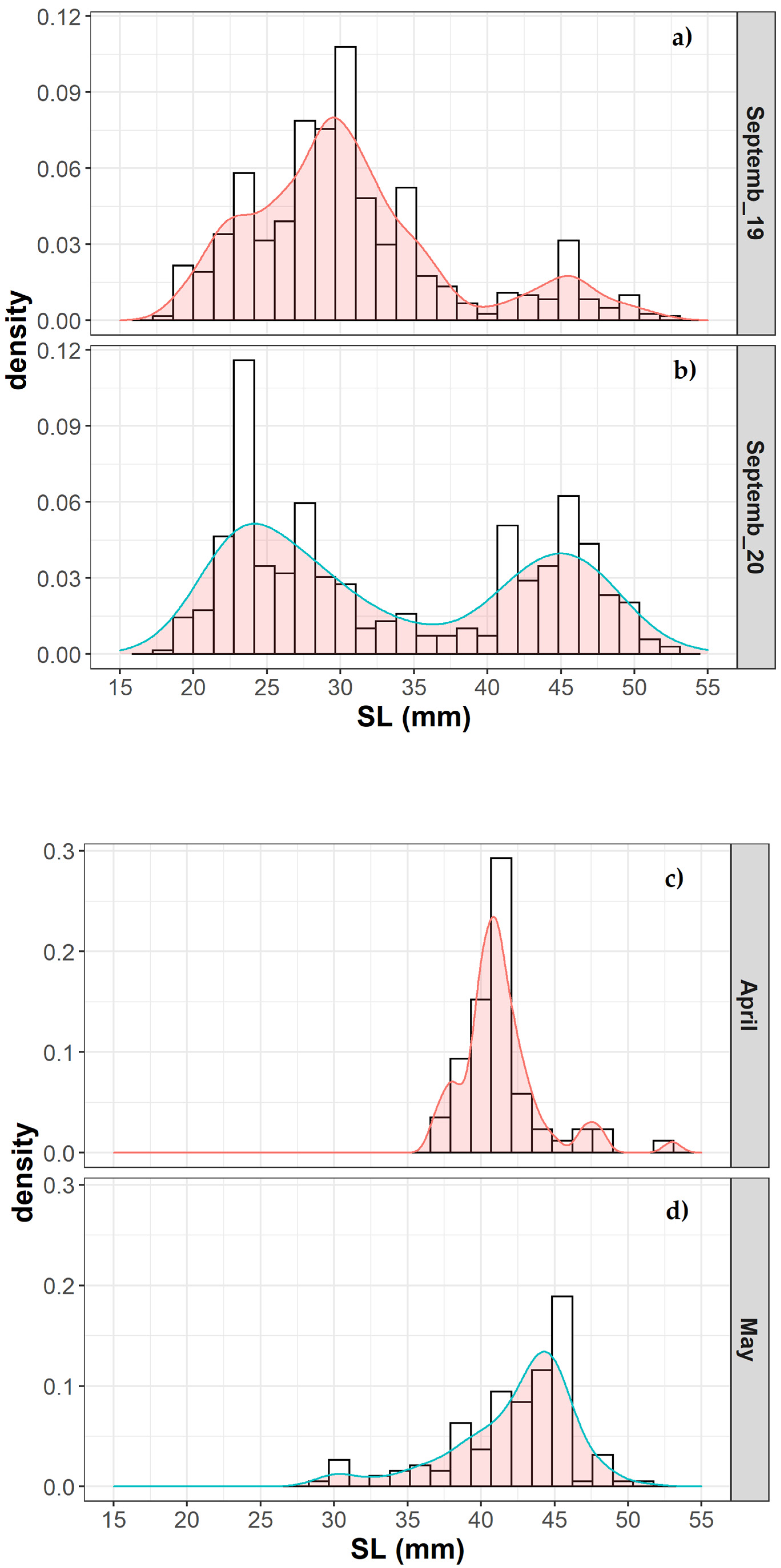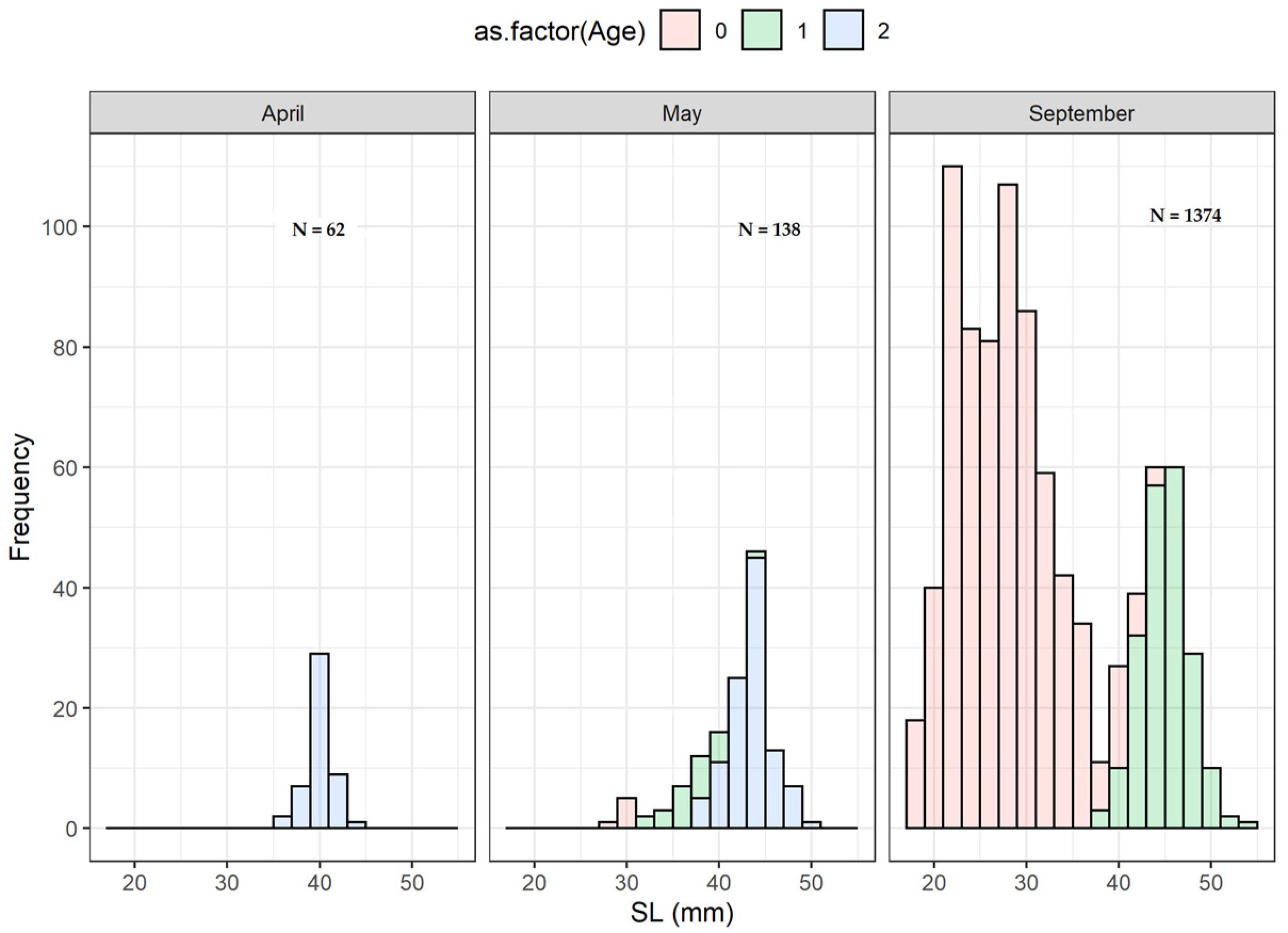However, despite this setback, we obtained estimates of key demographic parameters for the population of M. muelleri inhabiting the Bay of Biscay that largely resemble those previously reported for this species in other areas of the northeast Atlantic (as we discuss below). Based on three months of sampling and the size distribution and ages, we have been able to discern a temporal cycle for M. muelleri. Thus, the average length of the sampled individuals was different in spring and summer. While in September, most of the population consisted of juveniles (immatures, age group 0) or young adults (age group 1), adults dominated the population in April–May (mature, age groups 1 and 2).

In temperate and subtropical waters, M. muelleri generally spawns from late winter to early autumn (see

Table 10. Demographic parameters estimated/recorded for Maurolicus muelleri in this study and by various authors from different areas. BF = batch fecundity. When available, information on temperature and spawning season is also depicted. NA: Not applicable.

Area	BF (egg/g)	Fish Range (mm)	Max Age	Temperature	BF Method	Lfirst Mat	Spawning Season	Author
Southeast Australia	75–468	33.5–48.5	NA	NA	Number of oocytes > 500 um	32	July to October	Clarke 1982
Off Japan	109–333	42–48		NA		42	late winter to early spring	Okiyama, 1971
Norwegian waters	200–500	47–55	3	NA	Number of oocytes > 500 um	39	March to October	Gjosaeter, 1981
South Africa	161–738	10–52	NA	12–16.3 °C (100 m)	Number of oocytes in largest size class	24	all year, with peak in late winter/spring	Prost, 1991
Tasmania	104–942	34–54	NA	11.6–13.5 °C (200 m), 12–18 °C (Tsup)	Number of oocytes > 350 um	NA	NA	Young et al., 1987
South Africa	91–371	39–53	NA	NA	Number of oocytes > 500 um	NA	NA	Melo and Amstrong, 1991.
Rockall Trough	284–596	36.5–46.7	1?	9.5–13.5 °C (100 m)	NA	35	March to October	Kawaguchi and Mauchline, 1987
Norway waters	200–500	NA	NA	NA	Oocyte size distribution counting	NA	NA	Goodson et al., 1995
Bay of Biscay	114–919	41–51	2	12.6–21.1 °C (Tsup)	Hydrated oocyte method (>650 µm)	30	March to September	This study

). References are scarce for the Bay of Biscay, but eggs and larvae occur from February to June according to Valencia et al. [33], Rodriguez et al. [34], and Rodriguez [35]. In the survey data used for this study (JUVENA, MEGS, and BIOMAN surveys), early life stages were observed in March, April, and May, but not in September. However, mature individuals with spawning markers, i.e., hydrated oocytes, were found in September of 2020 (Table 7), indicating a spawning capability in late summer. Kawaguchi and Mauchline [13] identified a prolonged spawning season of about six months for this species in the area of Rockall Trough, describing the presence of juveniles in autumn and winter, mixed with late larvae or adults, respectively. The range of modes observed in the juvenile size distributions in September in the Bay of Biscay and the presence of juveniles in April suggest a potentially protracted spawning season. The poor representation of larger fish in late summer could be explained by different causes. On the one hand, M. muelleri are known to perform DVMs related to foraging [16]. DVMs were also detected in the Bay of Biscay [56], although our stomach content index did not mirror an obvious relation with the DVM, likely because of the absence of nocturnal samples (Figure S2). Some authors have found that larger adult fish do not perform DVMs [14,15], which could lead to reduced accessibility to these larger fish if the net does not reach the depth where they are found. This does not seem to be the situation in the Bay of Biscay, since the vertical distribution range of this species mainly comprises the first 400 m of the water column [56], which is usually sampled with the net. However, net avoidance may be higher at these size ranges than at smaller sizes (faster swimming of big-sized specimens), which would also contribute to a lower accessibility [57]. On the other hand, if the higher post-breeding mortality observed by Gjøsæter [28] in Norwegian waters also occurs in southern areas (as in Rockall Trough [13]), it would be expected that the proportion of adult fish of 1 or 2 years old in late summer would be reduced. Interannual differences can also occur, as reflected by the higher percentage of larger fish (SL > 40 mm, age group 1) in 2020 compared to 2019. In order to explain these differences, some hypotheses can be put forward. In line with the observations of other authors regarding post-spawning mortality, this interannual change in the adult fish proportion might be interpreted in terms of lower mortality rates for adult spawners in 2020 at the end of the spawning season. In this case, we might attribute particularly unfavourable post-spawning hydrographic conditions in one year compared to another as the driver of these changes. For instance, Rosland and Giske [58] stated that turbidity close to the surface would benefit M. muelleri, since the visibility of piscivores with long reaction distances would decrease more than the visibility of zooplanktivores with short reaction distances. The estimated wind-induced mixing in the Bay of Biscay for these years (Figure S3) showed no appreciable variability between years, so this mixing effect was insufficient to cause a singular effect on the M. muelleri mortality. An alternative hypothesis, and likely the simplest and most reasonable, is that differences in the population biomass are responsible for this perception (the estimates of biomass in the area were 157 and 208 ktons for 2019 and 2020, respectively—Guillermo Boyra, personal communication). Assuming a similar proportion of adults each year, it would be expected that the probability of catching adult fish in 2020 would be higher, as we indeed observed for this year.

4.1. Weight vs. Length

An analysis of the weight vs. length relationship is a rapid and simple way to describe several biological aspects of the species. Nevertheless, it also is known that these relationships are strongly affected by several factors; the factors that stand out as the most common are season, size range, and sex [59]. We observed interannual differences between both the coefficient of the slope (b) and the coefficient of the intercept (a). A higher “a” value in 2020 was interpreted as a better baseline condition of fish in that year, which could be a response to more favourable environmental conditions for growth in 2020 compared to 2019. The larger presence of adult fish in late summer with higher weights in 2020 than in 2019 supports this hypothesis of a better condition of fish, which would have a positive influence on their survival rates. Nevertheless, the indices of condition gave variable results. Fulton’s condition index increased in 2020 (10.6 vs. 9.8), providing new evidence of healthier fish in this year, while the Le Cren index (Knt) was not different between years.

The sex slightly modified the LW_evR of individuals, with females being heavier than males at larger sizes, although this result may have been influenced to some extent by the lower numbers of large males.

4.2. GSI and Sex Ratio

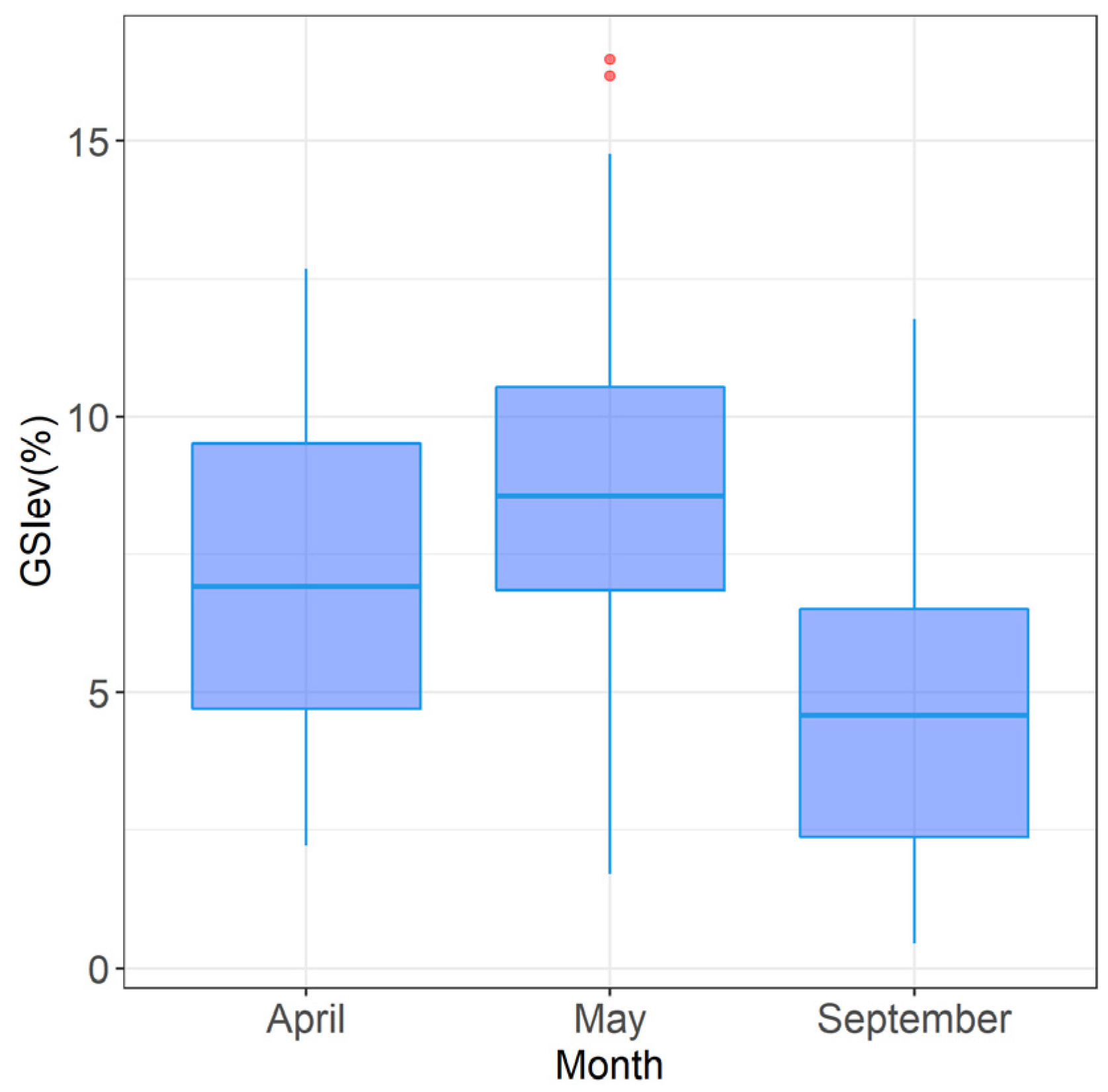
The range of values of the GSI estimated here was significantly higher than those described in the literature. The maximum value of the GSI (16%, in May) contrasts with those reported by Rasmussen and Giske [17] and Salvanes and Stockley [60] in Norway (7% and 5.6%, respectively), and Clark [6] in Australia (9.6%). Salvanes and Stockley [60] found that the highest averages for the GSI were closely related to the diameter of the oocytes, that is to say, to the maturation process of the fish gonads. 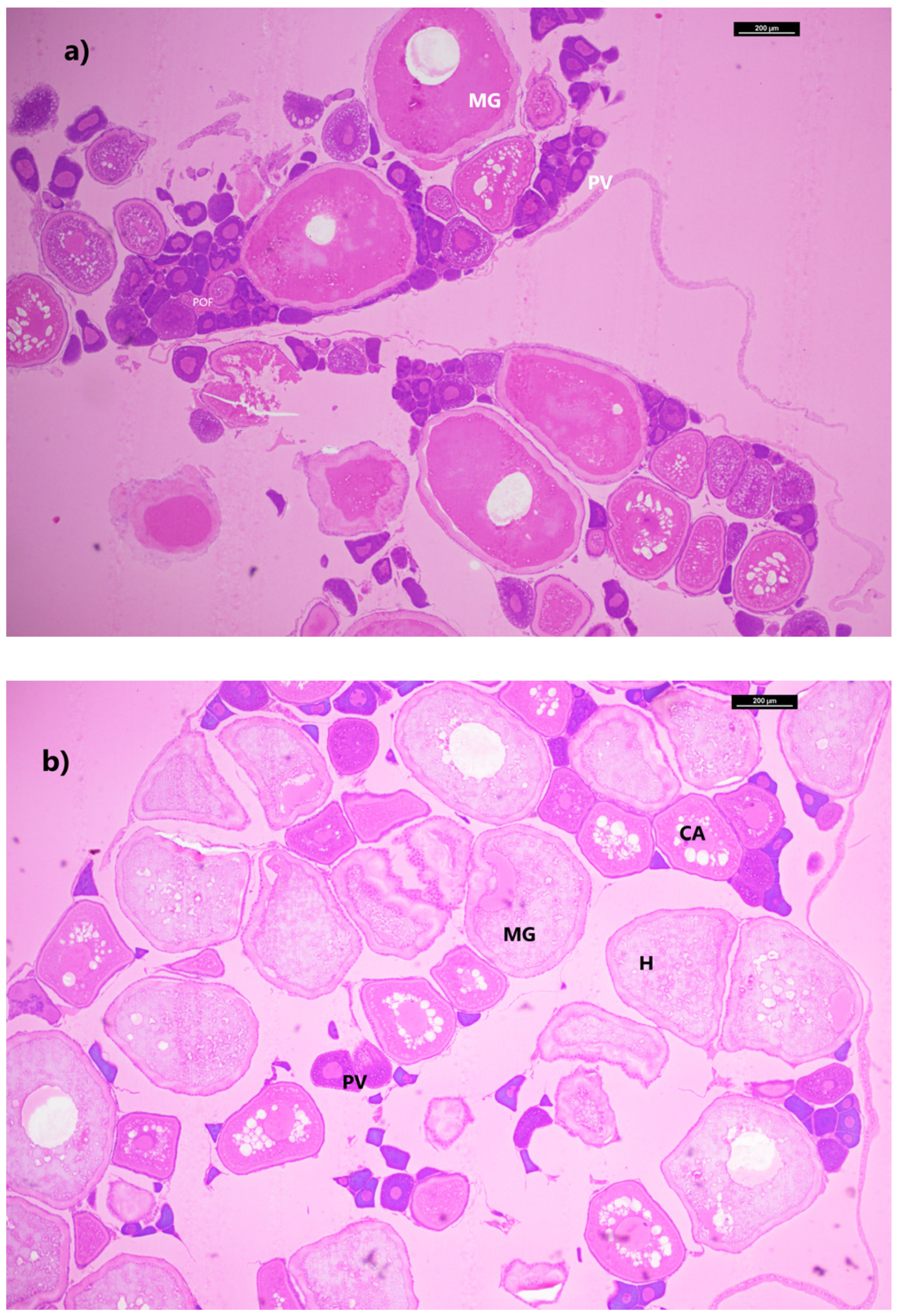In this study, the occurrence of fish with high GSI values (about 8%) in September as well denoted that a small proportion of M. muelleri exhibited reproductive activity in late summer. Higher GSI values in May indicated that there was a greater investment in reproduction during this period, which coincided with the presence of the more advanced stages of maturation in the gonad (Figure 6). This result demonstrates that the GSI may be used as a suitable tool for the evaluation of gonadal maturation in M. muelleri.

M. muelleri exhibits a positive bias in the ratio of females to males in larger fish groups [6,17,18,29,61]. In the samples taken in this study, males were most abundant at smaller size ranges, while females dominated progressively among larger sizes at a rate of 11% with the size. The overall ratio was slightly in favour of females at 0.44:0.56, whereas an equal proportion of males to females was predicted at 41.5 mm. Although this phenomenon seems to be common in mesopelagic species, it has not been observed in other populations of the same gender [62]. Different theories have been proposed to explain this difference in size. On the one hand, Rasmussen and Giske [17] suggested different mortality rates associated with sex or sexual differences in growth. On the other hand, Kristoffersen and Salvanes [61] proposed sex segregation by depth, which would change with age. More recently, Staby et al. [14] observed in Norwegian fjords that post-larvae and juvenile fish performed a normal crepuscular migration, while most of the adults remained at lower depths throughout the diel period. If male growth is lower than female growth, the juvenile phase of males should last longer, and the sex ratio should be in preference to juvenile males in the lower ranges. No clear evidence regarding a differential growth between sexes was found, probably because it was not possible to sex juvenile individuals. If there was vertical segregation by sex or size in the Bay of Biscay, sampling should cover the entire vertical distribution of the species to avoid bias in the sex ratio estimation. According to Sobradillo et al. [56], M. muelleri is preferentially distributed in a range of depths between 50 and 400 m, which corresponds to the usual depth at which the samples were taken in this study. Therefore, if one rules out these factors as likely to be responsible for the change in the sex ratio proportion by size, it seems that differential mortality may be the cause of the higher presence of females in larger fish groups.

4.3. Female Maturity

This is the first time that data on the reproductive parameters in terms of ovarian development, length at maturity, maturity ogive, and batch fecundity are presented for M. muelleri in the Bay of Biscay. The SL₅₀ was only slightly larger in females than in males (35.7 mm and 36.1, respectively) and somewhat lower in sex-combined than in sex-separated samples (34.1 mm). There is no information on this parameter for M. muelleri, but for sex-combined samples, our estimate for SL₅₀ was slightly larger than that of M. sthemanni (SL₅₀ = 32 mm), according to Almeida et al. [62]. The age and length at maturation show considerable variability within the same species, and this plasticity seems to be genetically defined and modelled by environmental variables [63]. For instance, the results showed that the size of the smallest mature female was 30 mm (by histological observation), which is within the range reported in the literature for different areas (20 to 40 mm [6,14,17,29,64,65,66,67]). Nevertheless, it would have been reasonable to expect a lower size at maturity in the Bay of Biscay if the sampling during the spawning peak (May or June) had been more intense, since in this period, reproductive activity occurs amongst individuals with a wider range of sizes [29].

Vazzoler (1996, in Almeida et al. [62]) defined the “critical minimum size” as the length at which the critical reproductive processes start, and proposed that species with a short life span and a small Lmax (r strategists), as is the case with M. muelleri, achieve mature gonadal stages before those species with a longer life span and a larger Lmax (k strategists).

The reproductive load (RL = Lm/Lmax) defines the relationship between the minimum size at maturation (Lm) and the maximum size a certain fish is likely to reach (Lmax). Froese and Binohland [68] compiled information from the literature for over 1100 fish and found that the Lm is, above all, a function of size. The values of these parameters are determined mainly by the interaction between the supply of oxygen and its demand [69]. According to these authors, the relationship varied between 0.4 and 0.9 and tended to be greater in smaller fish than in larger ones. With the aim of testing this hypothesis, we estimated this parameter (RL = 0.55) by taking the recorded minimum size at first maturation (SLm = 30 mm) and the maximum size observed (SLmax = 55 mm) of females as a reference. Our estimate was similar to the values reported by Almeida et al. [62] (Table 2) for the Maurolicus genus from different locations (about 0.5), with the exception of the populations located in Japan [64] and Tasmania [66]. This value is attributed to the ability of fish to perceive environmental stimuli that induce them to spawn [70]. This relationship seems to be genus-specific, so it will remain invariant within the same taxonomic group, and though environmental changes may cause modifications in both the SL₅₀ and SLmax, they will not influence the relationship between these parameters.

4.4. Fecundity Strategy

In general terms, fish undergo two types of fecundity: determinate and indeterminate [71], and reproductive parameters have to be estimated according to the reproductive strategy of the fish. In the case of determinate fecundity, all oocytes predestined to be spawned would be recognized at the beginning of the spawning season, and no new spawning oocytes would be recruited from the primary growth stocks, as is the case with indeterminate species [49]. Salvanes and Stockley [60] assumed an indeterminate fecundity for M. muelleri and estimated a total fecundity that ranged from 13,331 to 36,848 eggs in specimens from the northern Norwegian sea. Previously, Goodson et al. [29] found that the total fecundity of M. muelleri did not decrease when the spawning season progressed, indicating that new oocytes were being recruited. According to this evidence, M. muelleri should be regarded as an indeterminate species, and for that reason, the yearly fecundity should be calculated by estimating the spawning frequency, i.e., the percentage of females spawning per day, and the batch fecundity [51].

The batch fecundity was found to fluctuate greatly, both among individuals of the same population and between populations from different locations (Table 10). Our estimates of batch fecundity in May seem to be in the upper range of the values observed in different populations of this species distributed worldwide for individuals of a similar size (Table 10). This might mirror a differential life history strategy in the Bay of Biscay, where the fish, for the most part, seemingly reproduce no more than twice while alive and then die, while in other areas, fish live longer and take part in more than one spawning season. However, due to variations in the oocyte size thresholds used to determine the batch fecundity on the one hand, and the distinct range of fish analysed in each study on the other, the comparisons should be treated with caution.

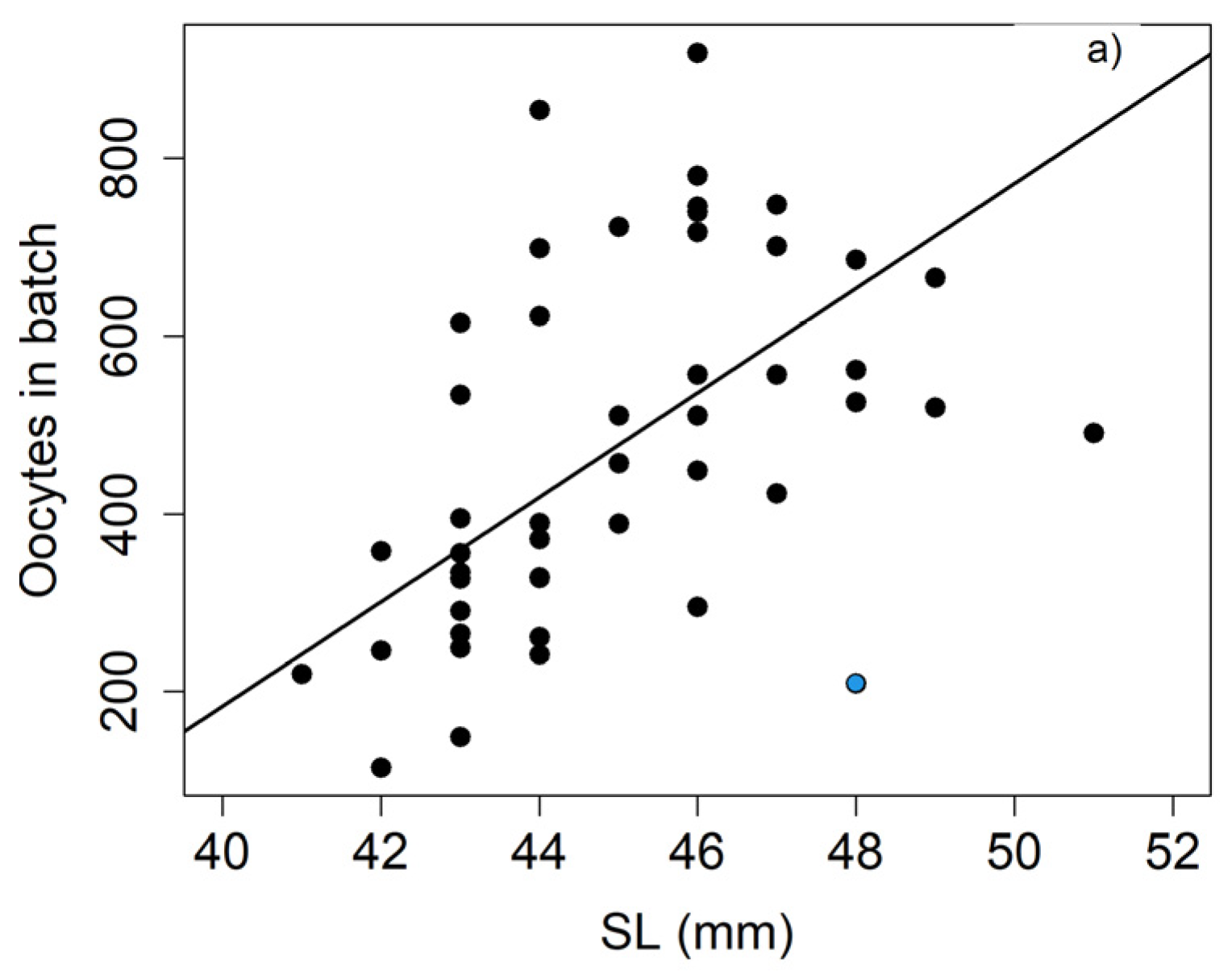
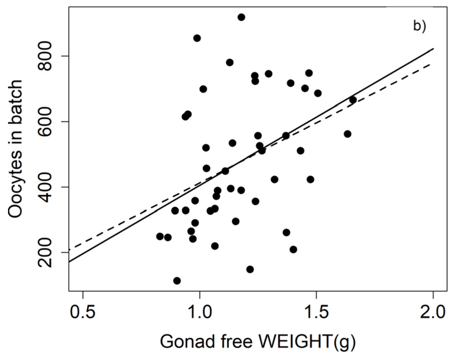
We found correlations between the batch fecundity and the size or weight, as has been found by other authors [6,13,17,72]. However, in other studies [2,8,12,66,67], no significant relationship between these variables was noticed. The lack of correlation between batch fecundity and size/weight could be attributed to different factors: firstly, because the range of weights is too short to obtain a relationship between the parameters, and secondly, due to the high dispersion of the batch fecundity, mainly in larger individuals. The high scatter amongst these individuals may indicate that these fish have already begun to spawn, diminishing their fecundity and increasing the variance in the data. This can be largely avoided by selecting only ovaries that do not present spawning markers, such as post-ovulatory follicles, as we did in this study. This seems to be the reason why we obtained a significant correlation, even though the range of fish sizes was narrow.

In this study, we provide some new insights into the biological sustainability of M. muelli as a basis for stock assessment in the Bay of Biscay. However, the exploitation of this resource is delicate and there is a lack of information in this regard. To date, no trial fishing for mesopelagic fish has been conducted in the Bay of Biscay, and it is unknown whether these species are captured as a bycatch and discarded by the trawling fleet that operate in this region. Further actions focused on these gaps are strongly recommended to prevent the misuse of this potential resource.

5. Conclusions

According to our findings, the population of M. muelleri in the Bay of Biscay is represented mostly by individuals of ages 0 and 1 in late summer (September) and age 2 in spring (April–May). While the age 2 group is absent in late summer, the age 1 fish represent a minor portion of the catches and could possibly be overrepresented, since mesh escapement is likely to be higher for the younger age 0 fish. Therefore, it appears that the number of fish surviving after spawning is low enough to offset poor recruitment in a given year. The length vs. weight relationships showed no clear differences by sex. The sex ratio was length-dependent, with larger fish being females. The batch fecundity was in the upper range of values compared to other world populations, which can be interpreted as a life history strategy of fish in the Bay of Biscay. In this area, most fish apparently spawn once and then die, while in other areas, they live longer and take part in more than one reproductive season. Consequently, a high mortality rate during the early life stages throughout the entire spawning season or the heavy exploitation of age 0 fishes before spawning could lead to a significant population decline from which recovery could be quite slow. Hence, if this population is ever exploited by a fishery, it should be regulated in such a way that fishing does not take place in an age 0 group before spawning.

References

1. Ramirez-Llodra, E.; Brandt, A.; Danovaro, R.; De Mol, B.; Escobar, E.; German, C.R.; Levin, L.A.; Martinez Arbizu, P.; Menot, L.; Buhl-Mortensen, P.; et al. Deep, diverse and definitely different: Unique attributes of the world’s largest ecosystem. Biogeosciences 2010, 7, 2851–2899. [Google Scholar] [CrossRef]
2. Gjøsæter, J.; Kawaguchi, K. A review of the world’s resources of mesopelagic fish. FAO Fish. Tech. Pap. 1980, 193, 1–151. [Google Scholar]
3. Sutton, T.; Clark, M.R.; Dunn, D.C.; Halpin, P.N.; Rogers, A.D.; Guinotte, J.; Bograd, S.J.; Angel, M.V.; Perez, J.A.A.; Wishner, K.; et al. A global biogeographic classification of the mesopelagic zone. Deep Sea Res. Part I Oceanogr. Res. Pap. 2017, 126, 85–102. [Google Scholar] [CrossRef]
4. Hays, G.C.; Graeme, C. A review of the adaptive significance and ecosystem consequences of zooplankton diel vertical migrations. In Migrations and Dispersal of Marine Organisms: Proceedings of the 37th European Marine Biology Symposium Held in Reykjavík, Iceland, 5–9 August 2002; Springer: Dordrecht, The Netherlands, 2003; pp. 163–170. [Google Scholar]
5. Robinson, C.; Steinberg, D.K.; Anderson, T.R.; Arístegui, J.; Carlson, C.A.; Frost, J.R.; Ghiglione, J.F.; Hernández-León, S.; Jackson, G.A.; Koppelmann, R.; et al. Mesopelagic zone ecology and biogeochemistry—A synthesis. Deep Sea Res. Part II Top. Stud. Oceanogr. 2010, 57, 1504–1518. [Google Scholar] [CrossRef]
6. Clarke, T.A. Distribution, Growth and Reproduction of the Lightfish Maurolicus muelleri (Sternoptychidae) off South-East Australia; CSIRO Marine Laboratories: Cronulla, NSW, Australia, 1982. [Google Scholar]
7. Prosch, R.M.; Shelton, P.A. The potential of lanternfish in broadening the base of the pelagic fishery. S. Afr. Shipp. News Fish. Ind. Rev. 1983, 38, 47–49. [Google Scholar]
8. Okiyama, M. Early life history of the gonostomatid fish, Maurolicus muelleri (Gmelin), in the Japan sea. Bull. Jpn. Sea Reg. Fish. Res. Lab. 1971, 23, 21–53. [Google Scholar]
9. Robertson, D.A. Planktonic stages of Maurolicus muelleri (Telestoi: Sternoptychidae) in New Zealand waters. N. Z. J. Mar. Freshw. Res. 1976, 10, 311–328. [Google Scholar] [CrossRef]
10. de Ciechmoski, J.D. Estudio de los huevos y larvas de la sardina fueguina Sprattus fueguensi y de Maurolicus muelleri, halllados en aguas adyacentes al sector Patagónico Argentino. Rev. Physis 1971, 30, 447–567. [Google Scholar]
11. Hulley, P.A.; Prosch, R.M. Mesopelagic fish derivatives in the southern Benguela region. S. Afr. J. Mar. Sci. 1987, 5, 597–611. [Google Scholar] [CrossRef]
12. Gjøsæter, J. Life history and ecology of Maurolicus muelleri (Gonostimatidae) in Norwegian waters. Fisk. Skr. Ser. Havunders. 1981, 17, 109–131. [Google Scholar]
13. Kawaguchi, K.; Mauchline, J. Biology of Sternoptychid Fishes Rockall lrough, Northeastern Atlantic Ocean. Biol. Oceanogr. 1987, 4, 99–120. [Google Scholar]
14. Staby, A.; Aksnes, D.L. Follow the light—diurnal and seasonal variations in vertical distribution of the mesopelagic fish Maurolicus muelleri. Mar. Ecol. Prog. Ser. 2011, 422, 265–273. [Google Scholar] [CrossRef]
15. Giske, L.; Dag, L.; Baliño, B.; Kaartvedt, S.; Lie, U.; Nordeide, J.; Salvanes, A.G.; Wakili, S.M.; Aadnesen, A. Vertical migration and trophic interaction of zooplankton and fish in Masfjorden, Norway. Sarsia 1990, 75, 65–81. [Google Scholar] [CrossRef]
16. Neilson, J.D.; Perry, R.I. Diel vertical migrations of marine fishes: An obligate or facultative process? Adv. Mar. Biol. 1990, 26, 115–168. [Google Scholar]
17. Rasmussen, O.I.; Giske, L. Life-history parameters and vertical distribution of Maurolicus muelleri in Masfjorden in summer. Mar. Biol. 1994, 120, 649–664. [Google Scholar] [CrossRef]
18. Bjelland, O. Life History Tactics of Two Fjordic Populations of Maurolicus muelleri. Master’s Thesis, University of Bergen, Bergen, Norway, 1995. [Google Scholar]
19. Irigoien, X.; Klevjer, T.A.; Røstad, A.; Martinez, U.; Boyra, G.; Acuña, J.L.; Bode, A.; Echevarria, F.; Gonzalez-Gordillo, J.I.; Hernandez-Leon, S.; et al. Large mesopelagic fishes biomass and trophic efficiency in the open ocean. Nat. Commun. 2014, 5, 3271. [Google Scholar] [CrossRef] [PubMed]
20. Anderson, T.R.; Martin, A.P.; Lampitt, R.S.; Trueman, C.N.; Henson, S.A.; Mayor, D.J. Quantifying carbon fluxes from primary production to mesopelagic fish using a simple food web model. ICES J. Mar. Sci. 2019, 76, 690–701. [Google Scholar] [CrossRef]
21. St John, M.A.; Borja, A.; Chust, G.; Heath, M.; Grigorov, I.; Mariani, P.; Martin, A.P.; Santos, R.S. A Dark Hole in Our Understanding of Marine Ecosystems and Their Services: Perspectives from the Mesopelagic Community. Front. Mar. Sci. 2016, 3, 31. [Google Scholar] [CrossRef]
22. Grimaldo, E.; Grimsmo, L.; Alvarez, P.; Herrmann, B.; Møen Tveit, G.; Tiller, R.; Slizyte, R.; Aldanondo, N.; Guldberg, T.; Toldnes, B.; et al. Investigating the potential for a commercial fishery in the Northeast Atlantic utilizing mesopelagic species. ICES J. Mar. Sci. 2020, 77, 2541–2556. [Google Scholar] [CrossRef]
23. Antarctic and Southern Ocean Coalition (ASOC). Illegal fishing threatens CCAMLR’s ability to manage Antarctica’s fisheries. Antarctica 1996, 5, 2. [Google Scholar]
24. Kock, K.-H. Understanding CCAMLR’s Approach to Management; CCAMLR: Hobart, Australia, 2000; p. 63. [Google Scholar]
25. Pauly, D.; Piroddi, C.; Hood, L.; Bailly, N.; Chu, E.; Lam, V.; Pakhomov, E.A.; Pshenichnov, L.K.; Radchenko, V.I.; Palomares, M.L.D. The Biology of Mesopelagic Fishes and Their Catches (1950–2018) by Commercial and Experimental Fisheries. J. Mar. Sci. Eng. 2021, 9, 1057. [Google Scholar] [CrossRef]
26. Albano, M.; D’Iglio, C.; Spanò, N.; Di Paola, D.; Alesci, A.; Savoca, S.; Capillo, G. New Report of Zu cristatus (Bonelli, 1819) in the Ionian Sea with an In-Depth Morphometrical Comparison with All Mediterranean Records. Fishes 2022, 7, 305. [Google Scholar] [CrossRef]
27. Childress, J.J.; Taylor, S.M.; Cailliet, G.M.; Price, M.H. Patterns of growth, energy utilization and reproduction in some meso- and bathypelagic fishes off southern California. Mar. Biol. 1980, 61, 27–40. [Google Scholar] [CrossRef]
28. Gjøsæter, J. Resource Studies of Mesopelagic Fish. Ph.D. Thesis, Department of Fisheries Biology, University of Bergen, Bergen, Norway, 1978. [Google Scholar]
29. Goodson, M.S.; Giske, J.; Rosland, R. Growth and ovarian development of Maurolicus muelleri during spring. Mar. Biol. 1995, 124, 185–195. [Google Scholar] [CrossRef]
30. Battaglia, P.; Malara, D.; Romero, T.; Andaloro, F. Relationships between otolith size and fish size in some mesopelagic and bathypelagic species from the Mediterranean Sea (Strait of Messina, Italy). Sci. Mar. 2010, 74, 305–6012. [Google Scholar] [CrossRef]
31. Nazir, A.; Khan, M.A. Stock-specific assessment of precise age and growth in the long-whiskered catfish Sperata aor from the Ganges River. Mar. Freshw. Res. 2020, 71, 1693–1701. [Google Scholar] [CrossRef]
32. Arbault, S.; Boutin, N. Ichthyoplankton oeufs et larves des poisons teleosteens dans le Golfe de Gascoyne en 1964. Rev. Des Trav. L’lnstitut Pech. Marit. 1968, 32, 413–476. [Google Scholar]
33. Valencia, V.; Motos, L.; Urrutia, J. Estudio de la variación temporal de la hidrografia y el plancton en la zona neritica frente a San Sebastián. Inf. Técnicos 1988, 20, 80. [Google Scholar]
34. d’Elbée, J.; Castège, I.; Hémery, G.; Lalanne, Y.; Mouchès, C.; Pautrizel, F.; D’Amico, F. Variation and temporal patterns in the composition of the surface ichthyoplankton in the southern Bay of Biscay (W. Atlantic). Cont. Shelf Res. 2009, 29, 1136–1144. [Google Scholar] [CrossRef]
35. Rodriguez, J.; Cabrero, A.; Gago, J.; Guevara-Fletcher, C.; Herrero, M.; de Rojas, A.H.; Garcia, A.; Laiz-Carrion, R.; Vergara, A.; Alvarez, P.; et al. Vertical distribution and migration of fish larvae in the NW Iberian upwelling system during the winter mixing period: Implications for cross-shelf distribution. Fish. Oceanogr. 2015, 24, 274–290. [Google Scholar] [CrossRef]
36. Rodriguez, J.M. Assemblage structure of ichthyoplankton in the NE Atlantic in spring under contrasting hydrographic conditions. Sci. Rep. 2019, 9, 8636. [Google Scholar] [CrossRef] [PubMed]
37. Punzón, A.; Serrano, A.; Sánchez, F.; Velasco, F.; Preciado, I.; González-Irusta, J.M.; López-López, L. Response of a temperate demersal fish community to global warming. J. Mar. Syst. 2016, 161, 1–10. [Google Scholar] [CrossRef]
38. Ortiz de Zarate, V. Datos sobre la alimentación del atun blanco (Thunnus alalunga, B.) juveniles capturado en el Golfo de Vizcaya. ICCAT Collect. Vol. Sci. Pap. 1987, 26, 243–247. [Google Scholar]
39. Pusineri, C.; Vasseur, Y.; Hassani, S.; Meynier, L.; Spitz, J.; Ridoux, V. Food and feeding ecology of juvenile albacore, Thunnus alalunga, off the Bay of Biscay: A case study. ICES J. Mar. Sci. 2005, 62, 11–22. [Google Scholar] [CrossRef]
40. Boyra, G.; Martinez, U.; Cotano, U.; Santos, M.; Irigoien, X.; Uriarte, A. Acoustic surveys for juvenile anchovy in the Bay of Biscay: Abundance estimate as an indicator of the next year’s recruitment and spatial distribution patterns. ICES J. Mar. Sci. 2013, 70, 1354–1368. [Google Scholar] [CrossRef]
41. ICES. Working Group on Mackerel and Horse Mackerel Egg Surveys (WGMEGS: Outputs from 2020 meeting). ICES Sci. Rep. 2021, 3, 88. [Google Scholar] [CrossRef]
42. ICES. Working Group on Southern Horse Mackerel Anchovy and Sardine (WGHANSA). ICES Sci. Rep. 2021, 3, 689. [Google Scholar] [CrossRef]
43. Campana, S.E. Photographic Atlas of Fish Otoliths of the Northwest Atlantic Ocean; NRC Research Press: Ottawa, ON, USA, 2004; p. 284. [Google Scholar]
44. Walsh, M.; Hopkins, P.; Witthames, P.R.; Greer Walker, M.; Watson, J. Estimation of Total potential Fecundity and Atresia in the Western Mackerel Stock in 1989; ICES Document CM; 1990; pp. 36–50. [Google Scholar]
45. Campana, S.E. Accuracy, precision and quality control in age determination, including a review of the use and abuse of age validation methods. J. Fish Biol. 2001, 59, 197–242. [Google Scholar] [CrossRef]
46. Morales-Nin, B. Determination of Growth in Bony Fishes from Otolith Microstructure; FAO Fisheries Technical Paper. No. 322; FAO: Rome, Italy, 1992. [Google Scholar]
47. Khan, M.A.; Nazir, A.; Khan, S. Assessment of Growth Zones on Whole and Thin-sectioned Otoliths in Sperata aor (Bagridae) Inhabiting the River Ganga, India. J. Ichthyol. 2016, 56, 242–246. [Google Scholar] [CrossRef]
48. ICES. Report of the Workshop on Age Reading of European Anchovy (WKARA), 9–13 November 2009, Sicily, Italy, ICES CM 2009/ACOM:43; 2010; pp. 9–13. Available online: https://doi.org/10.17895/ices.pub.19280525 (accessed on 27 February 2023).
49. Hunter, J.R.; Macewicz, B.J. Measurement of Spawning Frequency in Multiple Spawning Fishes; NOAA Technical Report NMFS. 36; US Department of Commerce: Springfield, VA, USA, 1985; pp. 79–93. [Google Scholar]
50. Aldanondo, N.; Cotano, U.; Goikoetxea, N.; Boyra, G.; Ibaibarriaga, L.; Iriogien, X. Interannual differences in growth and hatch-date distributions of early juvenile European anchovy in the Bay of Biscay: Implications for recruitment. Fish. Oceanogr. 2016, 25, 147–163. [Google Scholar] [CrossRef]
51. Hunter, J.R.; Nancy, C.H.L.; Leong, R.H. Batch Fecundity in Multiple Spawning Fishes; NOAA Technical Report NMFS. 36; US Department of Commerce: Springfield, VA, USA, 1985; pp. 67–77. [Google Scholar]
52. Silva, J.F.; Ellis, J.R.; Ayers, R.A. Length-weight relationships of marine fishes collected from around the British Isles. Sci. Ser. Tech. Rep. Cefas Lowestoft 2013, 150, 109. [Google Scholar]
53. Mozsár, A.; Boros, G.; Sály, P.; Antal, L.; Nagy, S.A. Relationship between Fulton’s condition factor and proximate body composition in three freshwater fish species. J. Appl. Ichthyol. 2015, 31, 315–320. [Google Scholar] [CrossRef]
54. Le Cren, E.D. The Length-Weight Relationship and Seasonal Cycle in Gonad Weight and Condition in the Perch (Perca fluviatilis). J. Anim. Ecol. 1951, 20, 201–219. [Google Scholar] [CrossRef]
55. Venables, W.N.; Ripley, B.D. Modern Applied Statistics with S, 4th ed.; Springer: New York, NY, USA, 2002; ISBN 0-387-95457-0. [Google Scholar]
56. Sobradillo, B.; Boyra, G.; Martinez, U.; Carrera, P.; Peña, M.; Irigoien, X. Target Strength and swimbladder morphology of Mueller’s pearlside (Maurolicus muelleri). Sci. Rep. 2019, 9, 17311. [Google Scholar] [CrossRef] [PubMed]
57. Kaartvedt, S.; Staby, A.; Aksnes, D. Efficient trawl avoidance by mesopelagic fishes causes large underestimation of their biomass. Mar. Ecol. Prog. Ser. 2012, 456, 1–6. [Google Scholar] [CrossRef]
58. Rosland, R.; Giske, J. A dynamic optimization model of the diel vertical distribution of a pelagic planktivorous fish. Prog. Oceanogr. 1994, 34, 1–43. [Google Scholar] [CrossRef]
59. Froese, R. Cube law, condition factor and weight–length relationships: History, meta-analysis and recommendations. J. Appl. Ichthyol. 2006, 22, 241–253. [Google Scholar] [CrossRef]
60. Salvanes, A.G.V.; Stockley, B.M. Spatial variation of growth and gonadal developments of Maurolicus muelleri in the Norwegian Sea and in a Norwegian fjord. Mar. Biol. 1996, 126, 321–332. [Google Scholar] [CrossRef]
61. Kristoffersen, J.B.; Salvanes, A.G.V. Sexual size dimorphism and sex ratio in Muller’s pearlside (Maurolicus muelleri). Mar. Biol. 2001, 138, 1087. [Google Scholar]
62. de Almeida, E.M.; del Bianco Rossi-Wongtschowski, C.L. Maurolicus stehmanni Parin & Kobyliansky, 1993 (Sternoptychidae): Length of first maturation, and spawning seasons in the south-southeast Brazilian region. Braz. J. Oceanogr. 2007, 55, 309–322. [Google Scholar]
63. Stearns, S.C.; Crandall, R.E. Plasticity for Age at Sexual Maturity: A Life-History Responses to Unavoidable Stress; Potts, G.W., Wootton, R.J., Eds.; Academic Press: Cambridge, MA, USA, 1984; pp. 13–33. [Google Scholar]
64. Yuuki, Y. Age and growth of a sternoptychid fish Maurolicus muelleri in the south western waters of the Sea of Japan. Bull. Jpn. Soc. Sci. Fish. 1982, 50, 1849–1854. [Google Scholar] [CrossRef]
65. Dalpadado, P.; Gjøsæter, J. Observations on mesopelagic fish from the Red Sea. Mar. Biol. 1987, 96, 173–183. [Google Scholar] [CrossRef]
66. Young, J.W.; Blaber, S.J.M.; Rose, R. Reproductive biology of three species of midwater fishes associated with the continental slope of eastern Tasmania, Australia. Mar. Biol. 1987, 95, 323–332. [Google Scholar] [CrossRef]
67. Prosch, R.M. Reproductive biology and spawning of the myctophid Lampanyctodes hectoris and the sternoptychid Maurolicus muelleri in the southern Benguela Ecosystem. S. Afr. J. Mar. Sci. 1991, 10, 241–252. [Google Scholar] [CrossRef]
68. Froese, R.; Binohlan, C. Empirical relationships to estimate asymptotic length, length at first maturity and length at maximum yield per recruit in fishes, with a simple method to evaluate length frequency data. J. Fish Biol. 2000, 56, 758–773. [Google Scholar] [CrossRef]
69. Longhurst, A.R.; Pauly, D. Ecology of Tropical Oceans; Academic Press: London, UK, 1987; p. 407. [Google Scholar]
70. Pauly, D. Gasping Fish and Panting Squids: Oxygen, Temperature and the Growth of Water-Breathing Animals; International Ecology Institute: Oldendorf, Germany, 2010. [Google Scholar]
71. Murua, H.; Saborido-Rey, F. Female reproductive strategies of marine fish species of the North Atlantic. J. Northwest Atl. Fish. Sci. 2003, 33, 23–31. [Google Scholar] [CrossRef]
72. Melo, Y.C.; Armstrong, M.J. Batch spawning behavior in lightfish Maurolicus muelleri. S. Afr. J. Mar. Sci. 1991, 10, 125–130. [Google Scholar] [CrossRef]
Figure 1. Spatial distribution of positive (crosses) and analysed (dots) hauls of M. muelleri during the JUVENA surveys in September of 2019 (black) and 2020 (red).
Hydrobiology 02 00019 g001
Figure 2. Length distribution of M. muelleri in (a) September of 2019 (n = 874), (b) September of 2020 (n = 500), (c) April of 2019 (n= 62), and (d) May of 2020 (n = 138).
Hydrobiology 02 00019 g002
Figure 3. Total weight (TW, gr) and standard length (SL, mm) relationship for M. muelleri in (a) 2019 and (b) 2020 by sex. 0 = undetermined, 1 = males, and 2 = females. Curves of the relationships are also shown. Table S2 shows the parameters and coefficients of the potential equations of TW vs. SL obtained for sex.
Hydrobiology 02 00019 g003
Figure 4. Plot of Fulton condition index (*106) with the SL (mm). Linear regression (blue line) and confidence intervals at 95% (grey shadow) are also shown. The linear equation parameters (±EE) and coefficient were Fulton = 9.545 (±0.135) + 0.017 (±0.003) ∗ SL (d.f. = 1572, R2adj = 0.011, p < 0.001). Red and blue dots refer to 2019 and 2020, respectively.
Hydrobiology 02 00019 g004
Figure 5. Boxplots of Le Cren index (Kn) calculated with (a) the total weight (Knt) and (b) the eviscerated weight (Kne) (bottom) by months. The values Sept_19 and Sept_20 refer to September of 2019 and 2020, respectively. Red points refer to outliers, the horizontal lines in the boxes refer to the median value of the index, and the length of the whiskers stands for the minimum and maximum values of the index.
Hydrobiology 02 00019 g005
Figure 6. Sections of ovarian histology, illustrating their seasonal aspects. (a) April: oocytes with multiple stages, MG, CA, and POFs (active spawning phase). (b) May: active developing reproductive phase, characterized by H and MG. (c) September 2019: immature-only PV oocytes. (d) September 2020: active developing reproductive phase, characterized by H and MG. PV = previtellogenic oocyte; CA = cortical alveolar oocyte; MG = migratory nucleus; POF = post-ovulatory follicle. Bar = 200 μm.
Hydrobiology 02 00019 g006aHydrobiology 02 00019 g006b
Figure 7. Boxplot of the gonadosomatic index (GSI) by month in the Bay of Biscay in 2019 and 2020, with the data combined. Red points refer to outliers, the horizontal lines in the boxes refer to the median value, and the length of the whiskers stands for the minimum and maximum values of the index.
Hydrobiology 02 00019 g007
Figure 8. Batch fecundity vs. (a) female SL and (b) female gonad free weight. The lines of the linear model (black plain) and generalized linear model (black dotted line) are shown. The dot in blue was deleted from the analysis. Details of the equation parameters are given in Table 9.
Hydrobiology 02 00019 g008aHydrobiology 02 00019 g008b
Figure 9. Length frequency distribution of the individuals captured in April, May, and September in the Bay of Biscay by age. N = number of samples examined.
Hydrobiology 02 00019 g009