Article

Predicting Habitat and Distribution of an Interior Highlands Regional Endemic Winter Stonefly (Allocapnia mohri) in Arkansas Using Random Forest Models

1
Department of Biological Sciences, University of Arkansas, Fayetteville, AR 72701, USA
2
Department of Entomology and Plant Pathology, University of Arkansas, Fayetteville, AR 72701, USA
3
U.S. Geological Survey, Arkansas Cooperative Fish and Wildlife Research Unit, Department of Biological Sciences, University of Arkansas, Fayetteville, AR 72701, USA
*
Author to whom correspondence should be addressed.
Hydrobiology 2023, 2(1), 196-211; https://doi.org/10.3390/hydrobiology2010013
Submission received: 15 December 2022 / Revised: 24 January 2023 / Accepted: 29 January 2023 / Published: 6 February 2023

Abstract

:
Stoneflies are a globally threatened aquatic insect order. In Arkansas, a diverse group of winter stonefly (Capniidae: Allocapnia) have not been surveyed since the 1980s, likely because species-level identification requires the rarely-collected adult form. Allocapnia mohri, a regional endemic, was previously commonly found in mountainous, intermittent streams from the Ouachita Mountains ecoregion north to the Ozark Highlands, but no species distributional models including land use or climate variables exist to our knowledge. We collected adults from 71 stream reaches from the historic Arkansas range from November to April 2020 and 2021. We modeled distributions using random forest (RF) models populated with landscape, climate, and both data to determine which were most predictive of species presence. Correlations between landscape or climate variables and presence were examined using multiple logistic regression. The landscape RF models performed better than the climate or landscape + climate RF models. A. mohri presence sites tended to have a greater elevation, a lower mean July temperature, and a greater percentage of very slow infiltration soils in the watershed, compared to absence sites. A. mohri was absent at the Ouachita Mountains sites and may be experiencing a range contraction or migration northward.

1. Introduction

Stoneflies (Plecoptera) are a highly diverse macroinvertebrate group encompassing more than 1000 species and representing 99 genera and ten families in North America [1]. Though the plecopteran group is expansive, little species-specific data on habitat, feeding habits, and distributions exist, and several existing records need updating to more accurately estimate their population status and to manage their conservation. This information is essential as Plecopterans are estimated to be one of the most endangered groups of insects globally [2,3]. Possible reasons for this include the alteration of plecopteran habitat by anthropogenic influences, such as climate and land use changes [3]. Here we model distributions of an endemic stonefly species to close the gap in species-specific stonefly knowledge, and to investigate whether climate, landscape, or a combination of factors could be affecting spatial distributions of stoneflies.
Several insect species, including the nymphs of some species of stonefly, are reliant on allochthonous resources [4], and the energy transported by these terrestrial materials, along with the energy acquired through autochthonous resources, is the primary source of matter and energy for many streams, particularly low order forested streams [5,6,7]. Shredding stoneflies will consume autumn-shed leaves, then these nymphs are subject to predation, thereby using the energy acquired through allochthonous sources. [8]. This cycling in of allochthonous material into the stream makes stoneflies a vital component of the stream food web [9]. The reliance on fallen leaves for food adds a habitat requirement of course particulate organic matter (CPOM) for shredder stoneflies in this macroinvertebrate group, and several stonefly species have strict water oxygenation and temperature requirements [10,11], increasing the habitat needs for these sensitive plecopteran nymphs. One such group of threatened plecopterans is the winter stonefly.
Stoneflies require specific environmental conditions, such as stream water temperatures and hydroperiod [12], and these factors will be affected by global climate change [13]. Ephemeroptera, Plecoptera, and Trichoptera (EPT) richness has displayed a decline of 81.6% worldwide, coming to an average loss of 1.9% loss of EPT richness each year. This 1.9% loss in richness mirrors the 1.88 °C increase in water temperature over the 40 years [14]. Several stonefly species have a thermal cue for egg hatching, and if stream temperatures do not reach a thermal low-end cue, nymphs will not hatch, causing extinction of species in certain thermally inadequate streams [12]. The effect of changing hydroperiod can greatly affect stoneflies, as they spend most of their lives as aquatic nymphs. Plecopterans are sensitive to benthic habitat loss, due in part to their need to lay eggs inside refugia within the stream (i.e., aquatic plants and woody debris), and their need to emerge using this refugia [12]. In some streams, stonefly nymphs can retreat to the hyporheic zone in dry periods, and it was found that several stonefly species even have diapausing eggs to outlast the dry stream conditions [15], though for many species and for many systems the hyporheic zone is not as important as refugia. Small stoneflies have been found to aggregate on stones, and larger stoneflies aggregate in leaf patches during high flow, as well as a general movement toward areas with flow in drying summer months [16].
Land-use change is another key driver of declines in stonefly populations [3]. Loss of riparian forest will likely amplify increases in stream water temperatures [17], reducing forested area in catchments, which may reduce stonefly habitat availability [18], and this, along with climate change, may cause reductions in stonefly populations due to their strict thermal requirements [10]. Further, standing crops of coarse benthic organic detritus can be directly related to the secondary production of shredding macroinvertebrates, such as stoneflies [19,20]. So, the loss of forested land in catchments can be strongly linked to a lower standing crop of litter detritus and likely reduced food availability for shredding stoneflies.
Forested land is often converted to agricultural or urban land uses that may also contribute to stonefly population declines and local species extinctions. Anthropogenic activities and land usage around stream systems directly influence the physical and chemical characteristics of the streams [21], including the amounts of sewage inputs, salts from road de-icing, and agricultural fertilizer and pesticides that seep into streams [22,23,24]. Anthropogenic activities can also result in impervious soil surrounding streams, leading to slow infiltration of water [25], causing an increase in speed and volume of storm runoff [26], and an increase in pollutants as a whole, ultimately causing a degradation of the aquatic habitat [27] and a loss of benthic macroinvertebrate diversity [28].
Anthropogenic nutrient inputs often lead to an increase in primary production [29], and this eutrophication can lead to low levels of dissolved oxygen (DO) during certain times of the day [29], thereby killing sensitive species in the stream, such as stoneflies [30]. This increase in nutrients can also stimulate microbial decomposition of leaf litter, the food source of shredders such as stoneflies [31]. While microbial colonization is thought to improve the nutritional quality of leaf litter for shredders, this is not always the case [32,33,34,35]. Further, elevated microbial decomposition may reduce the quantity of coarse detrital carbon available for food in stream ecosystems [36]. These effects can compound over time and be detrimental to stonefly species in the long-term.
Plecopterans are sensitive to these stream impurities and to microhabitat disturbances which makes them an important biological model to indicate water quality [37]. Most of the studies on benthic macroinvertebrates in relation to water quality evaluations have dealt with the richness of the EPT community because these groups are intolerant to pollutants in water bodies, but in the EPT community, Plecopterans are often the most sensitive to changes in water quality [38].
While the common causes of global-scale stonefly declines are known, a finer-scale, regional perspective is needed for conservation of sensitive groups, such as winter stoneflies. Winter stoneflies (Order: Plecoptera) emerge from the nymph stage in the winter months, and they are known as “clean-water insects’’ due to their need for highly oxygenated water [39]. A genus of winter stoneflies (Family: Capniidae, Genus: Allocapnia) emerges from the nymph stage to a small-winged adult across a wide variety of intermittent to perennial streams on vertical surfaces in and around the water body and lacks stream-to-stream vagility [12]. The Arkansas Level III Ecoregions known as the Ozark Highlands, Boston Mountains, Arkansas Valley, and Ouachita Mountains have a high diversity of Allocapnia. During the last regional census in the late 1980′s, seven endemic species of Allocapnia were found in Arkansas [12], several of which have recently been listed as species of greatest conservation need (SGCN) according to the Arkansas Game and Fish Commission’s 2019 Arkansas Wildlife Action Plan (AWAP).
A. mohri is a regional endemic that was commonly collected in the last 1980’s census [12], making it a good possible candidate for assessing important habitat factors and for distribution modeling. A. mohri populations during the previous census occurred broadly across Strahler stream orders one through five and were also found broadly across sites with differing flow permanence from intermittent sites with a completely dry stream bed or only pools with no flowing water for part of the year to perennial sites [12]. However, they were not detected at perennial sites with a significant groundwater flow [12]. This may be due to groundwater-based streams lacking the necessary temperature cue for egg hatching, whereas runoff dominated streams get cold enough with ice and snow melt entering the stream to cue hatching.
During the last widespread survey of Allocapnia in Arkansas, geospatial climate and land use data for stream catchments were not readily available [12] making it difficult to determine what factors are associated with A. mori distributions in the region. Species distribution models (SDMs) are empirical models relating field presence or abundance data to environmental predictor variables [40]. The use of SDMs has gained popularity in the past 20 years in ecological fields as geospatial mapping data with high resolution has become more readily available to conservation biology, making it possible to gauge the effect of climate, land use, and other environmental changes on the distribution of rare and understudied species [41].
One particular way of creating distribution maps that is gaining popularity is Random Forest (RF) modeling. Random Forest modeling is a group of tree predictors based on classification and regression tree (CART). The trees depend on the value of a random, independently sampled vector, so the method reduces bias [42]. Random Forest makes predictions by machine learning and then utilizes out-of-bag samples for model validation [43]. This method is excellent at minimizing overfitting due to its random nature and is effective at modeling spatial data even though it is not a spatial method. Random Forest modeling is superior to other popular SDM procedures, such as Mahalanobis Typicalities, a method adopted from remote sensing analyses. It is comparable to Maxent, a statistical mechanics approach, when one has a small-to-moderate number of the collected species presence/absence records (n = 38–94), and in species with low dispersal abilities [44]. The average number of records of each species of Allocapnia sampled in the previous census was 39 [12], and Plecoptera have reduced or absent flight capabilities, so Random Forest will likely work well for modeling winter stonefly species.
No SDMs exist for A. mohri to our knowledge. However, it was found to be the most widely distributed species of Allocapnia in Arkansas in the 1980’s (Figure 1A). Though this species used to be the most common through Arkansas, the species range has not been evaluated since the 1990s census. Also, due to the lack of geospatial data, no distribution models including land use and landcover or climate variables have been developed for A. mohri. Thus, our study objective was to recensus the Arkansas population and use the data to spatially model A. mohri distributions in Arkansas using RF models. Landscape, climate, and a combined landscape and climate data set were used to populate our RF model to determine which factors were most predictive of species presence. We then used multiple logistic regression to examine four hypotheses:
Hypothesis H1-A. mohri will be more likely to occur in mountainous regions and higher elevations [45]. Hypothesis H2-A. mohri will be more common in areas with high percentages of forested land [46] because leaf litter inputs are an important food source for detritivorous stoneflies [47]. Hypothesis H3-A. mohri will be more common in streams with high rainfall and low water temperatures [46]. Hypothesis H4-A. mohri will be less common in streams with a slow soil infiltration rate, due to their sensitivity to stream impurities [12].
Our resulting RF SDMs are some of the first published for a North American Plecopteran species (but see [48]), and the landscape RF model performed better than the climate or combined RF models. The MLR modeling indicated both landscape and climate variables were important for predicting presence. A. mohri was absent at the Ouachita Mountains sites in 2020 and 2021 possibly indicating range changes [12].

2. Materials and Methods
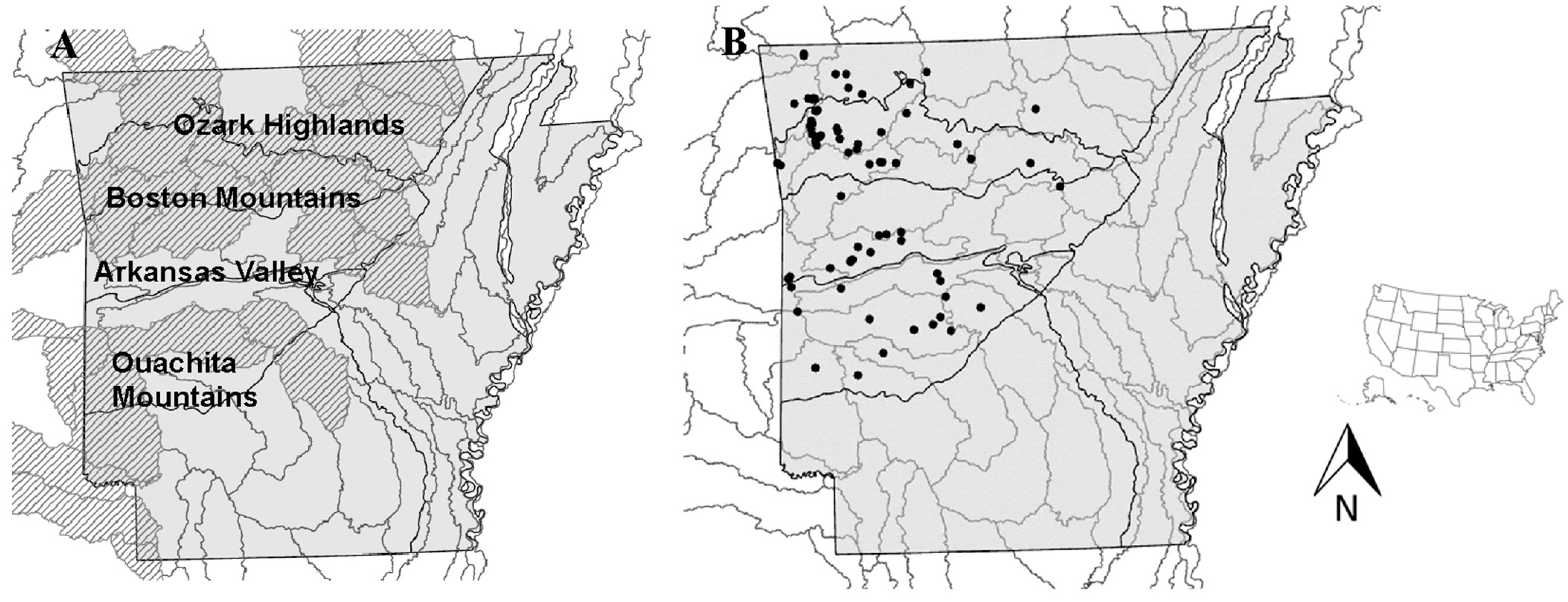
2.1. Study Design

Our study area included 73 sample reaches stratified across the Level II Ecoregion Ozark/Ouachita–Appalachian Forests, which lies within the Level I Ecoregion, the Eastern Temperate Forests. The sample reaches were further spread into the following Level III Arkansas Ecoregions: Ozark Highlands (n = 15), Boston Mountains (n = 29), Arkansas Valley (n = 13), and Ouachita Mountains (n = 16) (Figure 1). These Level III ecoregions historically had high stonefly diversity compared to other ecoregions in Arkansas [12]. Sample locations were based on historical studies reporting presence of Allocapnia genera [12]. We also stratified sample sites by Strahler stream order with several representing 1st order (n = 28), 2nd order (n = 15), 3rd order (n = 10), 4th order streams (n = 11), 5th order (n = 8), and 6th order (n = 1) (Table 1). Finally, the hydrologic flow regime was evaluated using the GeoCrawler Google Earth application (application located in Appendix B https://doi.org/10.1002/rra.2838, accessed on 1 January 2023). Due to the high amount of headwater streams sampled, and the stream locale belonging mainly to the Eastern Temperate Forests, most study sites had a high probability of belonging to the intermittent flashy flow regime (n = 46) [49].

2.2. Local Site Characterization

We measured the length and five wetted widths along evenly spaced transects for each habitat unit (e.g., riffles, pools, runs) at wadeable sites in August and September 2020–2022. Stream depth was measured at each width transect by taking five measurements across the cross-section of the stream. Each sample stream reach was 200 m in length, allowing all reaches to measure at least six times the wetted width of the stream, and each reach included at least one pool and riffle sequence [50]. Discharge was measured at the base of the reach using the mid-section method [51] at wadeable sites with no U.S. Geological Survey (USGS) gaging station. Otherwise, gaging station discharge was used.
Stream permanence was also estimated according to two separate metrics—one method described by Poulton and Stewart (1991) [12] and the other by Sheldon and Warren (2009) [52] in August and September of 2020–2022, which is generally the driest time of the year. The first method involved giving streams a ranking of A through D depending on the dryness over time, with an A ranking given to streams with a dry bed for part of the year and a D ranking given to streams with a permanent flow through the year along with a significant underground source. The second metric was a stream drying metric wherein we measured the linear extent of visible surface water in the stream reach in marked 50 m sections on each visit, then converted the wetted extent to a proportion, and calculated a time-weighted annual average for each site. This stream drying metric is primarily an index of time without surface flow, whereas the former gives a large-scale idea of the stream permanence. Using both metrics gives a clearer idea of the flow characteristics of each stream.

2.3. Landscape-Level Site Characterization

We collected two main types of landscape data: table and raster. Tabular climate and watershed data was collected virtually for all sites via Model My Watershed [53], and it was used in Multiple Logistic Regression (MLR) models (see Statistical analyses and modeling section). Several high-resolution landscape-level rasters were collected for the state of Arkansas to create distribution models of the species (see Statistical analyses and modeling section), including a land use raster (NLCD 2016) [54], a soil variable raster (gNATSGO) [55], and a large-scale environmental data raster (WorldClim) [56].

2.4. A. mohri Presence

Adult stonefly sampling started in early December and continued through mid-April during the 2020–2021 and 2021–2022 field seasons to match the emergence periods of A. mohri. Several approaches have been used to determine presence of Allocapnia populations in the past [12,52,57,58]. None of these methods have been evaluated to determine detection probability, which requires multiple samples over the emergence period. We chose to focus on adult collections, and all sample reaches were visited at least nine times across the emergence period to allow for evaluation of detection probability. We searched for adults in all areas of the 200 m reaches but particularly focused searches on compacted leaves and rocks in riffles, tree trunks, woody debris, and leaf litter debris piles on the side of the stream for 20 minutes per reach. All adults were collected by hand with forceps and immediately preserved in 95% ethanol, transported back to the laboratory, sexed, and identified to species using a regional taxonomic key [12]. The species were then placed on a distributional map.

2.5. Statistical Analyses and Modeling
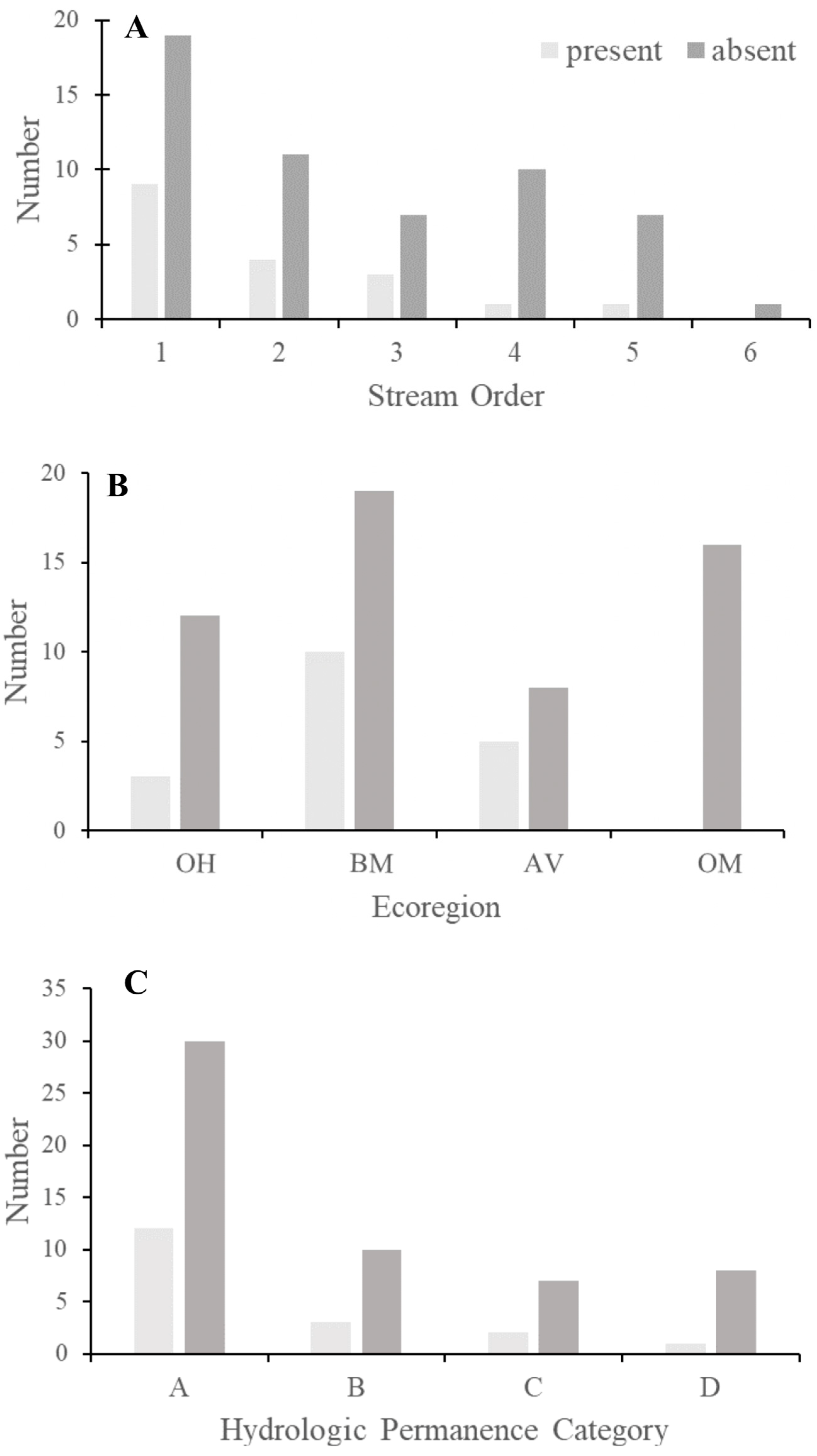
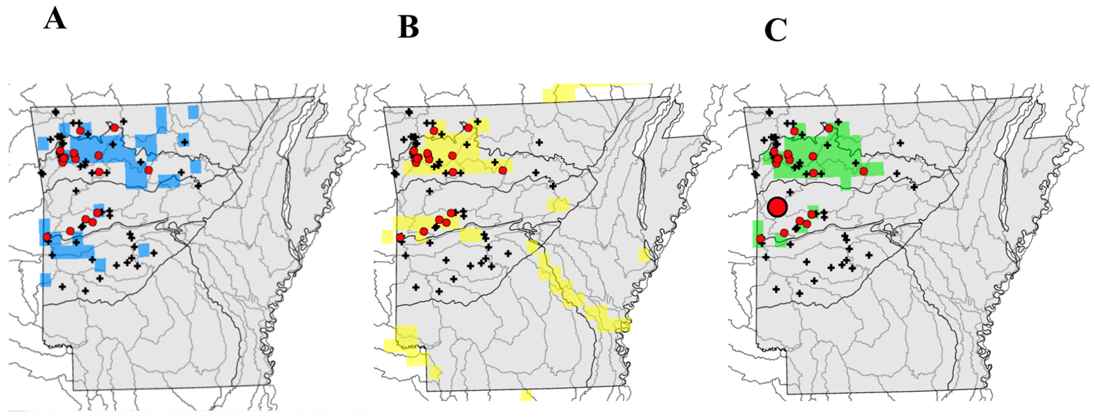
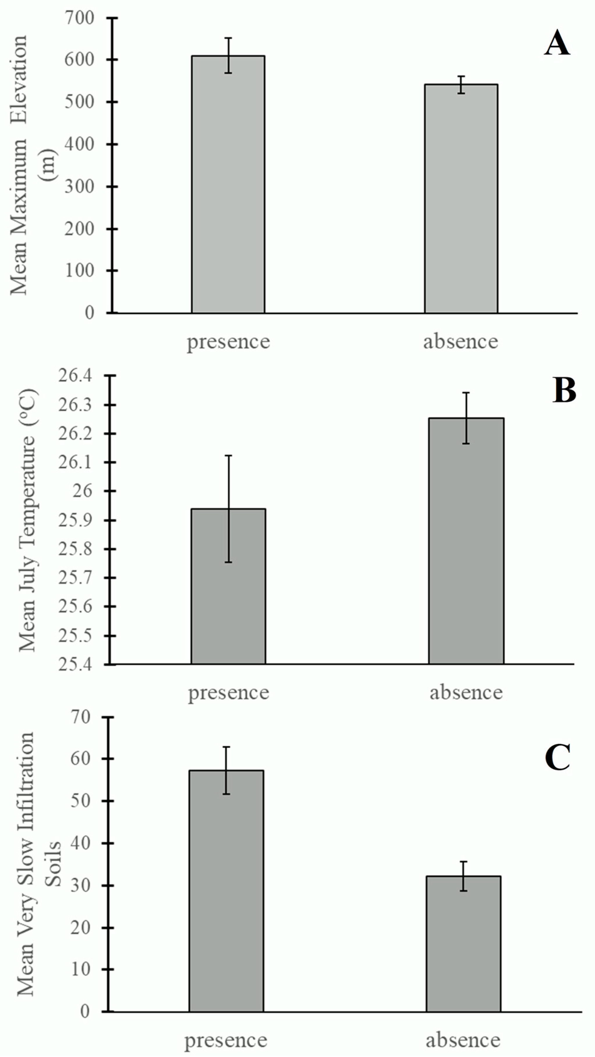
We chose Random Forest (RF) to determine the possible distribution of a species of Allocapnia mohri relative to using MaxEnt and Mahalanobis because of its reduced bias with moderate to large sample size and transparent readout [43]. The RF species distribution models in this study were created in ArcGIS [59], which also produced out-of-bag score, mean squared error, Matthews Correlation Coefficient, and F1 statistics to evaluate model accuracy. The out-of-bag (OOB) error is the average error for each tree, calculated using predictions from the trees that do not contain it in their respective bootstrap sample. This score provides information on the expected performance on new, unseen data, and generally, smaller OOB scores correspond with better models. The mean squared error (MSE) is a measure of the prediction accuracy of the model. There are no set acceptable limits for MSE, but in general the lower the MSE, the more accurate the model. F1 scores are a weighted average of the precision and recall of a model, where an F1 score reaches its best value at 1 and worst score at 0. The Matthews Correlation Coefficient scores are based on results for all four confusion matrix categories (true positives, false negatives, true negatives, and false positives), and a higher score corresponds to a better result. It scores proportionally both to the size of positive and negative elements in the dataset, making it a great metric for unbalanced data [60,61].
Three different RF models were created to parse out effects of land cover, soil, and climatic data. Each model was trained with 80% of the collected presence and absence data, and 20% of the data was used to validate and test the models. Model 1 was the “Landscape Model,” which included all land use and soil variable rasters along with an elevation raster. Model 2 was the “Climate Model,” which included only climatic raster data. Model 3 was the “Combined Model,” which included soil, land cover, and climatic variable rasters.
Random forest models are limited in that they do not depict the way that variables relate to one another, and they do not determine if the variables are significantly affecting A. mohri presence. Therefore, they are not appropriate for testing hypotheses about important habitat factors describing the landscape or climate niche of A. mohri in headwater streams. To resolve this issue, the data were evaluated using a multiple logistic regression (MLR). The MLR models were created in R (glm{stats}) [62]. A total of four separate models were created based on the four established hypotheses for this study (Table 2). The Hypothesis 1 (H1) model evaluated the ecoregion and elevation variables in the study to see if A. mohri was more common in mountainous regions and higher elevations. The Hypothesis 2 (H2) model included land use data to determine if A. mohri was more common in areas with a high percent of forested land. The Hypothesis 3 (H3) model included annual precipitation total and annual mean temperature variables to determine if A. mohri is more common in streams with high rainfall and low water temperatures. The Hypothesis 4 (H4) model included water infiltration rate variables to determine if A. mohri would be less common in streams with impacted soils. All landscape and climate predictor variables were tested for model assumptions including binomial distribution, independence of error terms, linear relationship between logit(Y) and X, and lack of collinearity among predictors. After checking for assumptions, some variables were excluded from analysis due to collinearity issues (correlation among predictor variables), and the variables that lacked logistic restraints and were determined to be of highest biological importance in the model were retained. All models were then compared and ranked using Akaike Information Criterion (AIC) to determine which model was best at predicting A. mohri presence, and Hosmer–Lemeshow goodness-of-fit tests and likelihood-ratio tests were run to compare all models to the global model.

3. Results

We collected and identified 3463 Allocapnia mohri individuals, with 2519 males and 944 females. This species began emerging around the end of November with the first A. mohri collection being made on 23 November 2020, nearly coinciding with the previously stated early December start of the emergence period for A. mohri [12]. We found A. mohri adults at 18 of our 73 sample reaches. Adults were found across stream orders one through five with no bias towards a particular stream order (Pearson’s chi-square = 3.42, p = 0.63, Figure 2A). A. mohri was not found at our 6th order stream site. A. mohri tended to be found in the Boston Mountains and Arkansas Valley ecoregions (Pearson’s chi-square = 0.25, p = 0.04, Figure 2B). Adults were also found across all hydrologic permanence categories with no bias towards a particular category (Pearson’s chi-square = 1.28, p = 0.73, Figure 2C).
Random Forest models estimated the potential distribution of Allocapnia mohri across Arkansas. The Landscape Model (Figure 3A) had an out-of-bag score of 0.594, an F1 score of 0.86, and MSE of 6.938, and a MCC of 0.83. Further evaluation of the visual present/absent prediction output of the RF model shows that 11 known present sites fall within the produced predicted bounds and 43 known absent sites correctly fall within the produced predicted absent bounds, meaning the visual prediction output for the Landscape model correctly sorted 54 present and absent sites out of 73 (73.9%).
The Climate Model (Figure 3B) had an out-of-bag score of 0.375, a F1 score of 0.80, a MSE of 11.008, and a MCC of 0.75 (Table 3). Further evaluation of the visual present/absent prediction output of this RF model shows that 15 known present sites fall within the produced predicted bounds and 42 known absent sites fall inside the produced predicted absent bounds, meaning the visual prediction output for the Climate model correctly sorted 55 present and absent sites out of 73 (78.1%).
The Combined Model (Figure 3C) had an out-of-bag score of 0.406, an F1 score of 0.57, a MSE of 9.631, and a MCC of 0.45 (Table 3). Further evaluation of the visual present/absent prediction output of this RF model shows that 15 known present sites fall within the produced predicted bounds and 38 known absent sites fall inside the produced predicted absent bounds, meaning the visual prediction output for the Landscape model correctly sorted 53 present and absent sites (72.6%).
Next, MLR models were used to test our study hypotheses. The H1 model showed total maximum elevation was significant in predicting A. mohri presence (p < 0.05, chi-square = 0.34), and elevation was positively correlated with species presence (Figure 4A, Table 4). The H2 model showed that no land use variable was significant in predicting A. mohri presence (p > 0.05; Table 4); however, there was a negative correlation between urban land and species presence. The H3 model showed that the hottest month temperatures were significant in predicting A. mohri presence (p < 0.05, chi-square = 0.34), and higher temperatures were negatively correlated with species presence (Figure 4B, Table 4). The H4 model was the best model according to AIC ranking. The results from the H4 model revealed that very slow soil infiltration was significant in predicting A. mohri presence (p < 0.01, chi-square = 0.53), and the correlation between A. mohri presence and very slow soil infiltration was positive (Figure 4C, Table 4). All MLR models were ranked using AIC, and the best MLR was found to be the H4 model (Table 4).

4. Discussion

Stoneflies are a major component to aquatic diversity [47]. Many species are globally imperiled [3,63], and yet little is known about species-specific habitat requirements and tolerances to changing land use and climate variables. Our study provides one of the first RF species distributional models for a North American plecopteran species. It also provides more detailed habitat and climate sensitivity information and updates distribution data that can aid conservation of a regional endemic winter stonefly species.
A 1980′s census provided some information about A. mohri‘s habitat [12] that is generally consistent with the present study’s findings, but our study adds to their results. We also found A. mohri broadly inhabited stream orders and hydrologic permanence categories. Specifically, A. mohri has been historically found at intermittent lower-order sites that have a completely dry stream bed or only have pools during parts of the year; therefore, they may have desiccation-resistant, diapausing eggs [64]. They also occurred at higher-order perennial sites; we found them at perennial sites that also have a significant underground spring source. A. mohri was historically found in first through fifth-order streams, but not in sixth-order streams. We found this same pattern. However, we only censused one sixth-order stream, which was located in the Ouachita Mountains. So, our study has limited power evaluating species presence in larger rivers.
Curiously, we did not find A. mohri in any of our 16 Ouachita Mountains stream reaches. A. mohri was found in Ouachita Mountains streams in the 1980′s [12]. Further, it was found in the Little Glazypeau Creek and Alum Fork of the Saline River drainages in 2000–2001 [52]. We have study reaches in these watersheds and did not find them despite visiting the reaches nine times during the winter emergence period. Their absence in the Ouachita Mountains ecoregion may be a statistical artefact, but it is possible that their southern range is shifting northward.
The Random Forest model using only landscape predictor variables was the best model of A. mohri distribution according to the OOB, MCC, F1, and MSE scores (Table 3). The Landscape model scored the highest in MCC out of all models and this metric in particular is an appropriate metric for this dataset, being that it works proportionally to the size of both positive and negative elements in the data, and the dataset that was used was uneven, with much more absence values than presence values. The Landscape model had the best accuracy in correctly predicting A. mohri absence when evaluating the incorrectly sorted present and absent sites in the RF prediction output. However, the Landscape model incorrectly sorted 19 present and absent sites out of the total 74 sample sites and incorrectly predicted that A. mohri should be present in the Ouachita Mountains ecoregion.
The Climate model was determined to be less accurate than the Landscape model according to the OOB, MCC, F1, and MSE scores, though it was the most accurate at sorting the present sites in the RF prediction output and had only 16 incorrectly sorted present and absent sites out of 74 sample sites. Though the Climatic model had the lowest OOB out of all three models, those scores test how accurately the model predicts the data it was given, meaning our Climate model did a great job in predicting the sites that we already knew about. The purpose of our distributional models was to predict the distribution of A. mohri outward into the rest of the state, which the Climate RF model does not do as well as the Landscape RF model, according to the other metrics used. The Climate model did correctly predict that A. mohri would not be present in the Ouachita Mountains ecoregion.
A. mohri tended to be present in watersheds with a greater maximum elevation (Figure 4, Table 3). Elevation is known to be an important component for plecopterans, as stonefly presence increases as elevation increases [12,45,65,66], and this is even true for rare stonefly species, like Beloneuria jamesae [67]. Elevation has also been found to be an important factor in stonefly abundance [45], showing that mountain streams are beneficial for plecopterans as a whole. The link between elevation and species presence could be due to high elevation streams being a lower stream size order (1–3) [68] with riparian vegetation contributing allochthonous inputs to the stream, which shredding macroinvertebrates utilize. The forested canopy also shades the stream and keeps water temperatures cooler compared to areas further downstream [69].
Stoneflies have been shown to be sensitive to stream temperature, and as water temperatures increase, streams become less hospitable to stoneflies [70]. Water temperature can be important to winter stonefly life cycles. For example, diapausing eggs may require a thermal cue to hatch [12]. Streams with average July temperatures reaching 26.4oC did not tend to have A. mohri present (Figure 4B). It is possible that these temperatures did not get low enough to cue eggs or nymphs [12]. Mean July and January temperatures increased as one moves from the Ozark Highlands south to the Ouachita Mountains ecoregion (Figure 5A and B, respectively). The Ouachita Mountains streams had a higher minimum and maximum mean temperature across the year than other ecoregions possibly explaining the absence of A. mohri. Higher elevation streams in the region may be a refuge from warmer stream temperatures [71]. However, the maximum elevation of our stream study reach watersheds was also the lowest in the Ouachita Mountains ecoregion (Figure 5B). Future studies should endeavor to sample some higher elevation streams in the Ouachita ecoregions to see if they might be A. mohri refuges. If these higher elevation streams act as shelter for temperature sensitive species, such as Allocapnia mohri, they might not be a haven for much longer. As climate change increases the temperatures of the vulnerable cool mountain streams, cold water adapted species like Allocapnia mohri will lose their thermal refuges [71] and eventually be replaced by more thermal generalist species, affecting the diversity of freshwater ecosystems [72,73,74,75].
Catchment soil infiltration category percentages were included in the best logistic model for predicting A. mohri presence (Table 2). This result may be due to the inherent soil texture found in each ecoregion. Soil texture refers to the percentage of sand, silt, and clay, which are the major factors affecting water infiltration. Species presence dropped to zero in the Ouachita Mountains ecoregion, which had the highest infiltration values of all visited ecoregions (Figure 5D). Soil in the Arkansas Valley, Boston Mountains, and Ozark Highlands ecoregions had a higher proportion of clay (a very small-pored soil) compared to the Ouachita Mountains, which has more sandy soil. Therefore, this correlation between very slow infiltration and species presence could just be due to the correlation between soil type and ecoregion.

5. Conclusions

Our resulting RF SDMs are some of the first published for a North American Plecopteran species. Though the landscape RF model performed better than the climate or combined RF models, our study indicates that climate and landscape factors are important habitat variables controlling A. mori distributions, as seen in our resulting MLR modeling, which suggested both landscape and climate variables were important for predicting presence. Even though landscape variables such as maximum elevation and soil infiltration categories led to strong models, these variables have likely not changed much over the last thirty years as A. mohri shifted from present to absent in censuses occurring in the Ouachita Mountains. The Landscape RF model also clearly predicts A. mohri should be present there, but the Climate RF model does not. Additional surveys for adults in the Ouachita Mountains stream reaches within predicted presence watersheds based on the RF model, particularly those with greater maximum elevation, could help determine if these reaches may be a refuge for A. mohri populations.
Climate change and associated warming stream waters can be a significant threat to macroinvertebrate taxa and can be responsible for species losses [3,65,70,76]. Warming stream temperatures may be causing losses of A. mohri in streams at the southern edge of its range (e.g., the Ouachita Mountains), shifting its distributions northwards. Evidence of range shifts due to effects of climate change has been observed in other macroinvertebrate species [75,77], and could be expected to occur for sensitive species in a continually warming climate.

Author Contributions

Conceptualization, M.A.E.-W., D.D.M., A.D., C.P. and B.A.; methodology, B.A., C.L. and M.A.E.-W.; formal analysis, B.A. and M.A.E.-W., writing—original draft preparation, B.A. and M.A.E.-W., writing—review and editing, M.A.E.-W., D.D.M., A.D., C.P. and C.L., funding acquisition, M.A.E.-W., D.D.M., A.D., C.P. and B.A., project administration, M.A.E.-W. All authors have read and agreed to the published version of the manuscript.

Funding

This project was funded by the State Wildlife Grants Program (Grant#AR-T-F19AF01234) of the U.S. Fish and Wildlife Service through an agreement with Arkansas Game and Fish Commission.

Institutional Review Board Statement

Not applicable.

Informed Consent Statement

Not applicable.

Data Availability Statement

Data available at https://github.com/mevanswh/ARstonefly_siteinfo (accessed on 1 January 2023).

Acknowledgments

We thank Zachary Tipton, Samuel Dias, Johnathan Novotny, Sahar Rezaei, Anthony Courter, Adam Annaratone, and Emily Carter for adult sampling help and comments on early drafts of this manuscript. Any use of trade, firm, or product names is for descriptive purposes only and does not imply endorsement by the U.S. Government. MEW can be contacted for the data.

Conflicts of Interest

The authors declare no conflict of interest.

References

  1. DeWalt, R.E.; Ower, G.D. Ecosystem Services, Global Diversity, and Rate of Stonefly Species Descriptions (Insecta: Plecoptera). Insects 2019, 10, 99. [Google Scholar] [CrossRef] [PubMed]
  2. Fochetti, R.; De Figueroa, J.M.T. Notes on diversity and conservation of the European fauna of Plecoptera (Insecta). J. Nat. Hist. 2006, 40, 2361–2369. [Google Scholar] [CrossRef]
  3. Sánchez-Bayo, F.; Wyckhuys, K. Worldwide decline of the entomofauna: A review of its drivers. Biol. Conserv. 2019, 232, 8–27. [Google Scholar] [CrossRef]
  4. Allan, J.D.; Castillo, M.M.; Capps, K.A. Stream Ecology: Structure and Function of Running Waters, 3rd ed.; Springer: Cham, Switzerland, 2021. [Google Scholar]
  5. Fisher, S.G.; Likens, G.E. Energy Flow in Bear Brook, New Hampshire: An Integrative Approach to Stream Ecosystem Metabolism. Ecol. Monogr. 1973, 43, 421–439. [Google Scholar] [CrossRef]
  6. Hornick, L.E.; Webster, J.R.; Benfield, E.F. Periphyton Production in an Appalachian Mountain Trout Stream. Am. Midl. Nat. 1981, 106, 22. [Google Scholar] [CrossRef]
  7. Martínez, A.; Larrañaga, A.; Pérez, J.; Basaguren, A.; Pozo, J. Leaf-litter quality effects on stream ecosystem functioning: A comparison among five species. Fundam. Appl. Limnol. 2013, 183, 239–248. [Google Scholar] [CrossRef]
  8. Perry, W.B.; Benfield, E.F.; Perry, S.A.; Webster, J.R. Energetics, Growth, and Production of a Leaf-Shredding Stonefly in an Appalachian Mountain Stream. J. N. Am. Benthol. Soc. 1987, 6, 12–25. [Google Scholar] [CrossRef]
  9. Thorp, J.H.; Rogers, D.C. Chapter 22—Stoneflies: Insect Order Plecoptera. In Field Guide to Freshwater Invertebrates of North America; Thorp, J.H., Rogers, D.C., Eds.; Academic Press: Boston, MA, USA, 2011; pp. 199–204. [Google Scholar]
  10. Zwick, P. Phylogenetic System and Zoogeography of the Plecoptera. Annu. Rev. Èntomol. 2000, 45, 709–746. [Google Scholar] [CrossRef] [PubMed]
  11. Maguire, T.J.; Mundle, S.O.C. Citizen Science Data Show Temperature-Driven Declines in Riverine Sentinel Invertebrates. Environ. Sci. Technol. Lett. 2020, 7, 303–307. [Google Scholar] [CrossRef]
  12. Poulton, B.C.; Stewart, K.W. The stoneflies of the Ozark and Ouachita Mountains (Plecoptera). Mem. Am. Entomol. Soc. 1991, 38, 1–116. [Google Scholar]
  13. IPCC, 2013: Climate Change 2013: The Physical Science Basis: Contribution of Working Group I to the Fifth Assessment Report of the Intergovernmental Panel on Climate Change; Cambridge University Press: Cambridge, UK; New York, NY, USA, 2013.
  14. Sánchez-Bayo, F.; Wyckhuys, K.A.G. Further evidence for a global decline of the entomofauna. Austral Èntomol. 2020, 60, 9–26. [Google Scholar] [CrossRef]
  15. Stanford, J.A.; Gaufin, A.R. Hyporheic Communities of Two Montana Rivers. Science 1974, 185, 700–702. [Google Scholar] [CrossRef]
  16. Lancaster, J.; Hildrew, A.G. Flow Refugia and the Microdistribution of Lotic Macroinvertebrates. J. N. Am. Benthol. Soc. 1993, 12, 385–393. [Google Scholar] [CrossRef]
  17. Pusey, B.J.; Arthington, A. Importance of the riparian zone to the conservation and management of freshwater fish: A review. Mar. Freshw. Res. 2003, 54, 1–16. [Google Scholar] [CrossRef]
  18. Burdon, F.J.; McIntosh, A.; Harding, J.S. Habitat loss drives threshold response of benthic invertebrate communities to deposited sediment in agricultural streams. Ecol. Appl. 2013, 23, 1036–1047. [Google Scholar] [CrossRef] [PubMed]
  19. Wallace, J.B.; Eggert, S.L.; Meyer, J.L.; Webster, J.R. Effects of Resource Limitation on a Detrital-Based Ecosystem. Ecol. Monogr. 1999, 69, 409–442. [Google Scholar] [CrossRef]
  20. Cross, W.F.; Wallace, J.B.; Rosemond, A.D.; Eggert, S.L. Whole-System Nutrient Enrichment Increases Secondary Production in a Detritus-Based Ecosystem. Ecology 2006, 87, 1556–1565. [Google Scholar] [CrossRef]
  21. Likens, G.E.; Bormann, F.H.; Johnson, N.M.; Fisher, D.W.; Pierce, R.S. Effects of Forest Cutting and Herbicide Treatment on Nutrient Budgets in the Hubbard Brook Watershed-Ecosystem. Ecol. Monogr. 1970, 40, 23–47. [Google Scholar] [CrossRef]
  22. Lee, J.-W.; Lee, S.-W.; An, K.-J.; Hwang, S.-J.; Kim, N.-Y. An Estimated Structural Equation Model to Assess the Effects of Land Use on Water Quality and Benthic Macroinvertebrates in Streams of the Nam-Han River System, South Korea. Int. J. Environ. Res. Public Health 2020, 17, 2116. [Google Scholar] [CrossRef]
  23. Waschbusch, R.J.; Selbig, W.; Bannerman, R.T. Sources of phosphorus in stormwater and street dirt from two urban residential basins in Madison. Wisconsin 1994, 95, 1999. [Google Scholar] [CrossRef]
  24. Omernik, J.M. The Influence of Land Use on Stream Nutrient Levels; US Environmental Protection Agency, Office of Research and Development, Corvallis Environmental Research Laboratory, Eutrophication Survey Branch: Corvallis, OR, USA, 1976. [Google Scholar]
  25. Paul, M.J.; Meyer, J.L. Streams in the Urban Landscape. In Urban Ecology: An International Perspective on the Interaction Between Humans and Nature; Marzluff, J.M., Shulenberger, E., Endlicher, W., Alberti, M., Bradley, G., Ryan, C., ZumBrunnen, C., Simon, U., Eds.; Springer US: Boston, MA, USA, 2008; pp. 207–231. [Google Scholar]
  26. Booth, D.B.; Jackson, C.R. Urbanization of Aquatic Systems: Degradation Thresholds, Stormwater Detection, and the Limits of Mitigation. JAWRA J. Am. Water Resour. Assoc. 1997, 33, 1077–1090. [Google Scholar] [CrossRef]
  27. Freeborn, J.R.; Sample, D.J.; Fox, L.J. Residential Stormwater: Methods for Decreasing Runoff and Increasing Stormwater Infiltration. J. Green Build. 2012, 7, 15–30. [Google Scholar] [CrossRef]
  28. King, R.S.; Scoggins, M.; Porras, A. Stream biodiversity is disproportionately lost to urbanization when flow permanence declines: Evidence from southwestern North America. Freshw. Sci. 2016, 35, 340–352. [Google Scholar] [CrossRef]
  29. Dodds, W.K. Trophic state, eutrophication and nutrient criteria in streams. Trends Ecol. Evol. 2007, 22, 669–676. [Google Scholar] [CrossRef]
  30. Stringfellow, W.; Herr, J.; Litton, G.; Brunell, M.; Borglin, S.; Hanlon, J.; Chen, C.; Graham, J.; Burks, R.; Dahlgren, R.; et al. Investigation of river eutrophication as part of a low dissolved oxygen total maximum daily load implementation. Water Sci. Technol. 2009, 59, 9–14. [Google Scholar] [CrossRef] [PubMed]
  31. Suberkropp, K. Annual production of leaf-decaying fungi in a woodland stream. Freshw. Biol. 1997, 38, 169–178. [Google Scholar] [CrossRef]
  32. Evans-White, M.A.; Haggard, B.E.; Scott, J.T. A Review of Stream Nutrient Criteria Development in the United States. J. Environ. Qual. 2013, 42, 1002–1014. [Google Scholar] [CrossRef] [PubMed]
  33. Halvorson, H.M.; Scott, J.T.; Sanders, A.J.; Evans-White, M.A. A stream insect detritivore violates common assumptions of threshold elemental ratio bioenergetics models. Freshw. Sci. 2015, 34, 508–518. [Google Scholar] [CrossRef]
  34. Howard-Parker, B.; White, B.; Halvorson, H.M.; Evans-White, M.A. Light and dissolved nutrients mediate recalcitrant organic matter decomposition via microbial priming in experimental streams. Freshw. Biol. 2020, 65, 1189–1199. [Google Scholar] [CrossRef]
  35. Eckert, R.A.; Halvorson, H.M.; Kuehn, K.A.; Lamp, W.O. Macroinvertebrate community patterns in relation to leaf-associated periphyton under contrasting light and nutrient conditions in headwater streams. Freshw. Biol. 2020, 65, 1270–1287. [Google Scholar] [CrossRef]
  36. Rosemond, A.D.; Benstead, J.P.; Bumpers, P.M.; Gulis, V.; Kominoski, J.S.; Manning, D.W.P.; Suberkropp, K.; Wallace, J.B. Experimental nutrient additions accelerate terrestrial carbon loss from stream ecosystems. Science 2015, 347, 1142–1145. [Google Scholar] [CrossRef] [PubMed]
  37. Stewart, K.W.; Stark, B.P. Plecoptera (Chapter 14). In An Introduction to the Aquatic Insects of North America, 4th ed.; Merritt, R.W., Cummins, K.W., Berg, M.B., Eds.; Kendall/Hunt Publishing Company: Dubuque, IW, USA, 2007; pp. 311–384. 1158p. [Google Scholar]
  38. Ab Hamid, S.; Rawi, C.S. Application of Aquatic Insects (Ephemeroptera, Plecoptera and Trichoptera) in Water Quality Assessment of Malaysian Headwater. Trop. Life Sci. Res. 2017, 28, 143–162. [Google Scholar] [CrossRef]
  39. McCafferty, W.P.; Provonsha, A.V. Aquatic Entomology: The Fishermen’s and Ecologists’ Illustrated Guide to Insects and Their Relatives; Jones and Barlett Publishers. Inc.: Boston, MA, USA, 1983. [Google Scholar]
  40. Guisan, A.; Zimmermann, N.E. Predictive habitat distribution models in ecology. Ecol. Model. 2000, 135, 147–186. [Google Scholar] [CrossRef]
  41. Guisan, A.; Thuiller, W. Predicting species distribution: Offering more than simple habitat models. Ecol. Lett. 2005, 8, 993–1009. [Google Scholar] [CrossRef]
  42. Breiman, L. Random forests. Mach. Learn 2001, 45, 5–32. [Google Scholar] [CrossRef]
  43. Breiman, L. Classification and Regression Trees, 1st ed.; Chapman & Hall/CRC: Boca Raton, FL, USA, 1984. [Google Scholar] [CrossRef]
  44. Hernandez, P.A.; Franke, I.; Herzog, S.K.; Pacheco, V.; Paniagua, L.; Quintana, H.L.; Soto, A.; Swenson, J.J.; Tovar, C.; Valqui, T.; et al. Predicting species distributions in poorly-studied landscapes. Biodivers. Conserv. 2008, 17, 1353–1366. [Google Scholar] [CrossRef]
  45. Grubbs, S.; Sheldon, A.L. The stoneflies (Insecta, Plecoptera) of the Talladega Mountain region, Alabama, USA: Distribution, elevation, endemism, and rarity patterns. Biodivers. Data J. 2018, 6, e22839. [Google Scholar] [CrossRef]
  46. Ross, H.H.; Ricker, W.E. The Classification, Evolution, and Dispersal of the Winter Stonefly Genus Allocapnia; University of Illinois Press: Urbana, IL, USA, 1971; Volume 45. [Google Scholar]
  47. Merritt, R.W.; Cummins, K.W.; Berg, M.B. An Introduction to the Aquatic Insects of North America, 5th ed.; Kendall/Hunt Publishing Company: Dubuque, IW, USA, 2019. [Google Scholar]
  48. Cao, Y.; DeWalt, R.E.; Robinson, J.L.; Tweddale, T.; Hinz, L.; Pessino, M. Using Maxent to model the historic distributions of stonefly species in Illinois streams: The effects of regularization and threshold selections. Ecol. Model. 2013, 259, 30–39. [Google Scholar] [CrossRef]
  49. Leasure, D.R.; Magoulick, D.D.; Longing, S.D. Natural Flow Regimes of the Ozark-Ouachita Interior Highlands Region. River Res. Appl. 2014, 32, 18–35. [Google Scholar] [CrossRef]
  50. Newbury, R.; Bates, D.; Alex, K.L. Restoring Habitat Hydraulics with Constructed Riffles. Earth Space Sci. 2013, 194, 353–366. [Google Scholar] [CrossRef]
  51. Gore, J.A. Chapter 3—Discharge Measurements and Streamflow Analysis; Academic Press: Cambridge, MA, USA, 2006. [Google Scholar]
  52. Sheldon, A.L.; Jr, M.L.W. Filters and templates: Stonefly (Plecoptera) richness in Ouachita Mountains streams, U.S.A. Freshw. Biol. 2009, 54, 943–956. [Google Scholar] [CrossRef]
  53. Stroud Water Research Center. Model My Watershed [Software]. 2020. Available online: https://wikiwatershed.org/ (accessed on 9 December 2022).
  54. Dewitz, J. National Land Cover Dataset (NLCD) 2016 Products; U.S. Geological Survey Data Release: Reston, VA, USA, 2019. [Google Scholar] [CrossRef]
  55. Soil Survey Staff, 2020. The Gridded National Soil Survey Geographic (gNATSGO) Database for Arkansas. United States Department of Agriculture, Natural Resources Conservation Service. 2020. Available online: https://nrcs.app.box.com/v/soils (accessed on 10 December 2022).
  56. Fick, S.E.; Hijmans, R.J. WorldClim 2: New 1-km spatial resolution climate surfaces for global land areas. Int. J. Climatol. 2017, 37, 4302–4315. [Google Scholar] [CrossRef]
  57. Tarter, D.C.; Chaffee, D.L.; Grubbs, S.A. Revised Checklist of The Stoneflies (Plecoptera) Of Kentucky, U.S.A. Entomol. News 2006, 117, 1–10. [Google Scholar] [CrossRef]
  58. McRoberts, T.; Grubbs, S. Effects of stream permanence on stonefly (Insecta, Plecoptera) community structure at Mammoth Cave National Park, Kentucky, USA. Biodivers. Data J. 2021, 9, e62242. [Google Scholar] [CrossRef] [PubMed]
  59. ArcGIS Pro, Version 2.7.2; ESRI: Redlands, CA, USA, 2020.
  60. Chicco, D.; Jurman, G. The advantages of the Matthews correlation coefficient (MCC) over F1 score and accuracy in binary classification evaluation. BMC Genom. 2020, 21, 6. [Google Scholar] [CrossRef]
  61. Boughorbel, S.; Jarray, F.; El Anbari, M. Optimal classifier for imbalanced data using Matthews Correlation Coefficient metric. PLoS ONE 2017, 12, e0177678. [Google Scholar] [CrossRef]
  62. R Core Team. R: A Language and Environment for Statistical Computing; R Foundation for Statistical Computing: Vienna, Austria, 2019; Available online: https://www.R-project.org/ (accessed on 4 December 2022).
  63. Reid, A.J.; Carlson, A.K.; Creed, I.F.; Eliason, E.J.; Gell, P.A.; Johnson, P.T.J.; Kidd, K.A.; MacCormack, T.J.; Olden, J.D.; Ormerod, S.J.; et al. Emerging threats and persistent conservation challenges for freshwater biodiversity. Biol. Rev. 2019, 94, 849–873. [Google Scholar] [CrossRef]
  64. Snellen, R.K.; Stewart, K.W. The Life Cycle of Perlesta placida (Plecoptera: Perlidae) in an Intermittent Stream in Northern Texas1. Ann. Èntomol. Soc. Am. 1979, 72, 659–666. [Google Scholar] [CrossRef]
  65. Sheldon, A.L. Possible climate-induced shift of stoneflies in a southern Appalachian catchment. Freshw. Sci. 2012, 31, 765–774. [Google Scholar] [CrossRef]
  66. Garcia-Raventós, A.; Viza, A.; de Figueroa, J.M.T.; Riera, J.L.; Múrria, C. Seasonality, species richness and poor dispersion mediate intraspecific trait variability in stonefly community responses along an elevational gradient. Freshw. Biol. 2017, 62, 916–928. [Google Scholar] [CrossRef]
  67. Sheldon, A.L.; Grubbs, S.A. Distributional ecology of a rare, endemic stonefly. Freshw. Sci. 2014, 33, 1119–1126. [Google Scholar] [CrossRef]
  68. Strahler, A.N. Quantitative analysis of watershed geomorphology. Eos Trans. Am. Geophys. Union 1957, 38, 913–920. [Google Scholar] [CrossRef]
  69. Vannote, R.L.; Minshall, G.W.; Cummins, K.W.; Sedell, J.R.; Cushing, C.E. The River Continuum Concept. Can. J. Fish. Aquat. Sci. 1980, 37, 130–137. [Google Scholar] [CrossRef]
  70. Hotaling, S.; Shah, A.A.; Dillon, M.E.; Giersch, J.J.; Tronstad, L.M.; Finn, D.S.; Woods, H.A.; Kelley, J.L. Cold Tolerance of Mountain Stoneflies (Plecoptera: Nemouridae) from the High Rocky Mountains. West. N. Am. Nat. 2021, 81, 54–62. [Google Scholar] [CrossRef]
  71. Mulholland, P.J.; Marzolf, E.R.; Webster, J.R.; Hart, D.; Hendricks, S.P. Evidence that hyporheic zones increase heterotrophic metabolism and phosphorus uptake in forest streams. Limnol. Oceanogr. 1997, 42, 443–451. [Google Scholar] [CrossRef]
  72. Burgmer, T.; Hillebrand, H.; Pfenninger, M. Effects of climate-driven temperature changes on the diversity of freshwater macroinvertebrates. Oecologia 2006, 151, 93–103. [Google Scholar] [CrossRef] [PubMed]
  73. Durance, I.; Ormerod, S.J. Climate change effects on upland stream macroinvertebrates over a 25-year period. Glob. Chang. Biol. 2007, 13, 942–957. [Google Scholar] [CrossRef]
  74. Hering, D.; Schmidt-Kloiber, A.; Murphy, J.; Lücke, S.; Zamora-Muñoz, C.; López-Rodríguez, M.J.; Huber, T.; Graf, W. Potential impact of climate change on aquatic insects: A sensitivity analysis for European caddisflies (Trichoptera) based on distribution patterns and ecological preferences. Aquat. Sci. 2009, 71, 3–14. [Google Scholar] [CrossRef]
  75. Domisch, S.; Jähnig, S.C.; Haase, P. Climate-change winners and losers: Stream macroinvertebrates of a submontane region in Central Europe. Freshw. Biol. 2011, 56, 2009–2020. [Google Scholar] [CrossRef]
  76. Shokri, M.; Cozzoli, F.; Vignes, F.; Bertoli, M.; Pizzul, E.; Basset, A. Metabolic rate and climate change across latitudes: Evidence of mass-dependent responses in aquatic amphipods. J. Exp. Biol. 2022, 225, jeb244842. [Google Scholar] [CrossRef]
  77. Pélissié, M.; Johansson, F.; Hyseni, C. Pushed Northward by Climate Change: Range Shifts With a Chance of Co-occurrence Reshuffling in the Forecast for Northern European Odonates. Environ. Èntomol. 2022, 51, 910–921. [Google Scholar] [CrossRef] [PubMed]
Figure 1. (A) Historic distribution of A. mohri across Omernik Level III ecoregions. The HUC8 units that overlapped with A. mohri presence watersheds from Poulton and Stewart, 1991 are hatched. The HUC8 units in Arkansas that did not have A. mohri presence are outlined. (B) Locations of the 74 reaches sampled in the present study. The northernmost site coordinates are (36.44117572, −94.22998045) southernmost site coordinates are (34.68526175, −94.32049797). Sample reaches fell within the following HUC8 units: Ouachita Headwaters, Upper Saline, Fourche La Fave, Poteau, Petit Jean, Frog-Mulberry, Dardanelle Reservoir, Robert S. Kerr Reservoir, Beaver Reservoir, Bull Shoals Lake, Elk, Little Red, Middle White, Buffalo, Upper Ouachita, Little Missouri, Lower Little, Illinois.
Hydrobiology 02 00013 g001
Figure 2. The distribution of A. mohri present and absent sites across stream orders (A), Omernik level III Ecoregions (B) of Ozark Highlands (OH) Boston Mountains (BM), Arkansas Valley (AV), and Ouachita Mountains (OM), and Hydrologic Permanence Categories (C); Poulton and Stewart, 1991).
Hydrobiology 02 00013 g002
Figure 3. The Random Forest distribution models for Allocapnia mohri plotted with the known species distribution. A. mohri presence (red circle) and absence (+) sites are marked. The areas that the Landscape distribution model predicted would have A. mohri presence are marked in blue (A). The areas that the Climate distribution model predicted would have A. mohri presence are marked in yellow (B). The combined Landscape and Climate model prediction is in green (C).
Hydrobiology 02 00013 g003
Figure 4. The mean and standard error of maximum watershed elevation (A), July temperatures (B), and the percentage of very fine soils in the watershed (C) for sites where Allocapnia mohri was present and absent.
Hydrobiology 02 00013 g004
Figure 5. The mean + 1SE of July (A) and January (B) stream temperatures during our study period and of the maximum elevation (C) and percentage of very slow infiltration soils (D) in study reach catchments grouped by ecoregions. Ecoregions move from north (left) to south (right). OH = Ozark Highlands, BM = Boston Mountains, AV= Arkansas Valley, OM = Ouachita Mountains.
Hydrobiology 02 00013 g005
Table 1. The range, median, and mean of each variable across our study sites.
VariablesRangeMedianMean
Stream Order1st–6th22.48
Mean Width (m)0.66–6.522.62.99
Mean Depth (cm)5.56–41.4014.7215.63
Elevation (m)155–598401370.37
%Forested8.61–98.686.2576.26
%Agriculture0.00–51.577.7412.62
%Urban0.23–57.735.0310.75
%High Infiltration Soils0.00–66.762.324.36
%Moderate Infiltration Soils0.00–84.2119.2524.79
%Low Infiltration Soils0.00–100.0016.8227.04
%Very Slow Infiltration Soils0.00–96.1038.1538.31
Total Annual Precipitation (cm)110.0–155.3127.1125.7
Total February Precipitation (cm)5.9–10.87.97.9
Total May Precipitation (cm)12.6–17.514.714.8
Annual Mean Water Temperature (°C)14.2–16.914.715.2
January Mean Water Temperature (°C)2.1–5.62.83.4
July Mean Water Temperature (°C)25.1–27.625.926.2
Table 2. Variables used in Multiple Logistic Regression analyses grouped by hypothesis. N/A indicates that no variable was removed from the final model due to correlation and/or collinearity.
ModelVariablesRemoved Due to Correlation and/or Collinearity
H1 ModelEcoregion, Elevation, Average Elevation, Max Elevation, Min ElevationAverage Elevation, Min Elevation, Elevation
H2 Model%Forest, %Agriculture, %UrbanN/A
H3 ModelAnnual Precip Total (cm), Annual Mean Temp (°C), July Mean Temp, Jan Mean Temp, May Total Precip, Feb Total PrecipAnnual Mean Temp, Jan Mean Temp, May Total Temp, Feb Total Precip
H4 ModelHigh Infiltration, Moderate Infiltration, Slow Infiltration, Very Slow InfiltrationSlow Infiltration
Table 3. Random Forest model scores for Out-of-Bag (OOB), F1, Mean Squared Error (MSE), Matthews Correlation Coefficient (MCC), Accuracy, and Validation Accuracy variables used in Multiple Logistic Regression analyses grouped by hypothesis.
ModelOut of Bag ScoreF1 ScoreMSEMCCAccuracyValidation Accuracy
Model 1: Landscape0.5940.866.940.830.920.75
Model 2: Climate0.3750.811.0080.750.920.88
Model 3: Climate + Landscape0.4060.579.6310.450.910.62
Table 4. Results from the Multiple Logistic Regression (MLR) showing values for p and chi-square, then Akaike Information Criterion (AIC) ranking for four hypotheses related to Allocapnia mohri presence/absence.
ModeldfChi-Squaredp-ValueAIC Score
H1 Model30.34p < 0.0580.37
H2 Model20.23p > 0.0583.36
H3 Model20.31p < 0.0580.35
H4 Model20.53p < 0.0173.49
Disclaimer/Publisher’s Note: The statements, opinions and data contained in all publications are solely those of the individual author(s) and contributor(s) and not of MDPI and/or the editor(s). MDPI and/or the editor(s) disclaim responsibility for any injury to people or property resulting from any ideas, methods, instructions or products referred to in the content.

