1. Introduction
Axisymmetric nozzle jets are a significant type of free shear layer flows that exhibit turbulence. The primary phenomenon is turbulence caused by the velocity gradient and instabilities between the jet and the surrounding fluid [
1]. Reactive flows are recognized as beneficial constituents of turbulent jets and are extensively employed in diverse sectors, including combustion and military engineering. The complexity of addressing these jets stems from the interaction between turbulent mixing and heat release caused by chemical reactions [
2,
3].
The process of modeling turbulent reacting flows relies numerically on models that were originally developed for constant-density flows that do not involve any chemical reactions. The efficacy of utilizing said models may be inadequate in terms of authenticity. The utilization of a turbulent, non-reacting variable-density jet can streamline the issue at hand while retaining the intricacy of variable density. This approach also eliminates the requirement to account for the interplay between turbulent mixing and chemical heat release, as stated in reference [
3]. Numerous experimental investigations have been carried out on turbulent jets with constant density, as documented in references [
4,
5,
6,
7,
8]. Several experiments have been conducted on strongly variable-density jets using axisymmetric nozzles, as documented in references [
9,
10,
11,
12,
13,
14,
15,
16,
17]. Advanced laser technology has facilitated a comprehensive analysis of the reactive behavior of turbulent jets, as reported in references [
18,
19].
The inlet conditions, including injection ratio, co-flow direction, and nozzle geometry, have an impact on the features of variable-density turbulent jets [
2,
20]. The injection ratio is a key parameter that has a significant impact on the initial mixing and subsequent development of a jet [
20]. It is defined as the ratio of the momentum flux of the jet to that of the ambient fluid. According to reference [
2], the flow structure, turbulence levels, and mixing processes within a jet can be modified by the direction and magnitude of the co-flowing fluid, thereby influencing the behavior of the jet. The behavior of a jet is significantly impacted by the geometry of its nozzle, which affects both its initial velocity and turbulence intensity. The development of a jet, specifically its entrainment and spread, can be influenced by the shape of the nozzle, as documented in reference [
2]. The precise modeling and forecasting of turbulent jets with variable densities necessitate meticulous attention to inlet conditions. Understanding the influence of these factors on the dynamics of jet flow and turbulent mixing is essential for a range of industrial applications, such as combustion, mixing, and heat transfer processes. The study of the effects of inlet conditions on variable-density turbulent jets is a prominent area of research that can provide valuable insights into the complex behavior of these flows.
Gonçalves et al. performed numerical simulations of a turbulent non-premixed, and non-reacting Propane jet flow in the presence of co-flowing air using the Unsteady Reynolds Averaged Navier-Stokes (URANS) modeling and Standard k-ε model. Furthermore, they used an adaptive refinement in the mesh domain to reduce the computational cost. They finally compared numerical results for velocity and mixture fraction at the jet center line with experimental data for validation and observed a satisfactory performance of their approach [
21].
The spatial development of air-air compressible coaxial jets was numerically simulated by Ouzani R et al. using 3D-Monotone Integrated Large Eddy Simulations (MILES). The computations were performed on isothermal and non-isothermal coaxial jets. The spatiotemporal evolution of the mixture fraction field is utilized to track the mixing between inner and outer jets. The spatially developing approach is a method that considers the various phases of turbulent mixing, including molecular diffusion, transition, and fully developed turbulent state. The results obtained were found to be satisfactory and in good agreement with the experimental data. The examination of mixture fraction fluctuations suggests that the onset of turbulent mixing occurs earlier in the non-isothermal scenario. The statement is consistent with the early formation of the Kelvin–Helmholtz vortices [
22].
The objective of this study is to assess the efficacy of the Realizable k-ε eddy viscosity turbulence model in reproducing the outcomes of experiments conducted on a turbulent axisymmetric jet. The objective was achieved by utilizing and modifying one of the standard solvers in OpenFOAM 5 (i.e., ReactingFoam) with the assistance of SWiss Army Knife for Foam (Swak4Foam). The reactingFoam is intended to tackle mixing issues in compressible flows that involve combustion and reactions. The performance of the model can be assessed and confirmed by simulating the experimental data obtained from the TNF data archive, which can be accessed at
http://www.sandia.gov/TNF/DataArch/ProJet.html (accessed on 10 March 2023).
The Realizable k-ε turbulence model is a well-established and widely employed model in the field of fluid dynamics for the purpose of forecasting turbulent flows. This model has been validated and is frequently utilized for the prediction of turbulent jets that do not involve any chemical reactions [
1]. The employed model is a modified variant of the Standard k-ε model. It accounts for the influence of turbulence anisotropy and compressibility. The methodology utilized is founded upon the Reynolds-Averaged Navier-Stokes (RANS) equations. The model effectively resolves intricate turbulence structures and mixing processes occurring within the jet, thereby offering significant insights into flow dynamics and turbulent mixing phenomena. The Realizable k-ε eddy viscosity turbulence model, in conjunction with numerical simulations, provides a cost-effective and efficient method for investigating turbulent axisymmetric jets. The aforementioned approach offers significant advantages over experimental research as it enables accurate control of inlet conditions and overcomes practical constraints inherent in physical experiments. The results of this study can assist in improving the accuracy and reliability of computational tools used for predicting turbulent jet dynamics. The aforementioned can result in noteworthy consequences for diverse industrial implementations.
In the present numerical study, the Realizable k-ε eddy viscosity turbulence model with two equations was utilized for the first time in this specific test case. The model was used to simulate turbulent flow on an approximate 2D plane (specifically a 5-degree partition of the cylinder of the experimental domain). The simulation was conducted using OpenFOAM 5 and the swak4Foam utility, with the reactingFoam solver being meticulously manipulated. The initial step for modeling a turbulent axisymmetric jet in this research involved selecting the sandiaD_LTS tutorial (located in combustion > reactingFoam > RAS) to begin the process of manipulating the numerical test cases. The tutorial case concerns a reacting flow, but the study has excluded combustion and chemical reaction from the experiment as they are not observed. The reactingFoam solver’s robust features were utilized to achieve a precise simulation of a non-reacting jet through this methodology. The accuracy and reliability of the selected modeling approach can be assessed by comparing the simulation outcomes with the experimental data.
3. Description of Computational Domain and Assumptions
The axisymmetric assumption is deemed reasonable based on a comparison between the inner and outer dimensions of the tube and the horizontal cross-section of the experimental domain. Additionally, the significant difference in bulk velocity between Propane and co-flowing air supports this assumption. This hypothesis has the potential to decrease the computational resources needed substantially. The computational domain is constrained to a nearly 2D plane, which is precisely a sector of the 5-degree of the largest cylinder that can be embedded in the real domain.
There are two distinct approaches to the preparation of computational geometry. In the first one, the sector can be defined by disregarding the length of the nozzle. Consequently, the simulation will not include the flow inside the nozzle. In this scenario, the inlets for Propane and co-flowing air will be located at the level of the nozzle exhaust.
In the other approach (as in this study), an alternative method was employed, similar to the other approach, where a 10 cm nozzle was placed upstream to aid in achieving fully developed flow within the nozzle. Pre-injection was performed to improve the development of the boundary layer between the co-flowing air and the outer edge of the nozzle, as observed during experimentation. This was performed before injecting the mixture into the main computational domain. The primary approach is characterized by reduced cell quantities, resulting in cost-effectiveness and efficiency. However, it may exhibit lower precision levels as it may not entirely replicate the actual boundary conditions that surround the nozzle’s structure.
The Realizable k-ε model utilizes a variable function for the coefficient C
µ in the equation for turbulent viscosity (v
t), which distinguishes it from the Standard k-ε model where C
µ is a constant. The transport equation governing Turbulence Kinetic Energy (k) is the same in both the Standard and Realizable k-ε models, except for variations in model constants. The transport equation for Dissipation Rate (ε) has been modified by segregating it from the precise equation for the transportation of mean-square vorticity fluctuations. The aforementioned modification is significant. The Realizable k-ε model outperforms all other versions of the k-ε models in accurately predicting the spreading rate of planar and round jets [
24].
The computational domain in this study has been restricted to a distance of 100 cm (x/D = 190), as determined by the graphical representation of the experimental data. No significant variations were detected beyond the value of x/D greater than 80. The co-flowing air is composed of N2 and O2 with volume fractions of 0.7632 and 0.2368, respectively. It is assumed that the flow is compressible and isothermal at a temperature of 294 K. The injected fluid is considered to be an ideal gas.
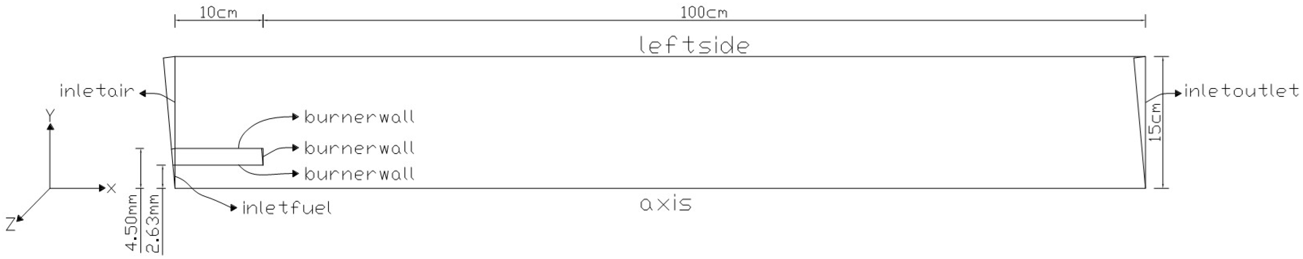
The system folder contains the blockMeshDict, changeDictionaryDict, and extrudeMeshDict files. The simulation domain’s boundaries were established and modified through the utilization of the blockMeshDict file and its corresponding files for each variable located in the 0 folders. The boundaries of the system are defined as follows: inletfuel, which represents the inlet boundary of Propane upstream on the inner diameter of the nozzle; inletair, which represents the inlet boundary of co-flowing air at the upstream, from the outer ridge of the nozzle to the lateral border on the left side; outlet, which represents the downstream outlet boundary; axis, which represents the symmetry axis for sector rotation; leftside, which represents the lateral edge of the domain; burnerwall, which represents the part of upstream boundaries that represents the nozzle body; and front and back, which are used for simulating a 2D problem.
A simplified scheme of the computational domain is depicted in
Figure 1. It should be noted, X, Y and Z are the selected axes in the modeling and solution process throughout the paper.
The grids were adjusted in the X and Y directions of each block in the blockMeshDict file using a predefined lengthGrading. This was performed to reduce computational costs and achieve a suitable aspect ratio.
The calculation of turbulence kinetic energy, denoted as k, can be achieved through the following formulations:
However, based on the experimental data, it is suggested that a 2D assumption can be made, resulting in a simplification of the model to
Non-dimensional parameters were plotted at the outset. An assessment was performed on the axial and radial profiles of various parameters, including average velocities, turbulence energy, average mixture fraction, and a half radius of the mixture fraction. Subsequently, the pressure (p) was demonstrated in the results. A figure is presented to compare the obtained Total Kinetic Energy, k, results for all four test cases. The comparison is made at the center line and at x/D values of 15, 30, and 50. A comparison was made between the numerical and experimental data for every parameter.
Table 1 provides a concise presentation of the computational domain’s dimensions and inlet data:
4. Initial and Boundary Conditions of Variables
The meshes provided indicate that the final computational node located on the leftside will be positioned beyond the boundary layer. It is crucial for the accuracy of the wall functions assumption that Y-plus is not restricted to a range of 30 to 100. Therefore, the utilization of wall functions is prohibited. However, for reasons of numerical cost, it is not advisable to increase the mesh resolution towards the outer walls, specifically the leftside.
The initial method involves adopting a boundary condition of fixedValue, with a value of 9.2 assigned to the velocity variable U, while the other variables are subjected to a zeroGradient boundary condition. The leftside boundary is subjected to a simulated slip condition in an attempt to closely approximate reality. It is expected that the meshes have undergone adequate refinement on both the inner and outer surfaces of the nozzle body, particularly on the burnerwall. The variables alphat, epsilon, k, and nut were subjected to a wall function, whereas U was subjected to a no-slip condition.
Furthermore, a secondary method was utilized to authenticate the accuracy of the assumptions made regarding the burnerwall of the nozzle. The process required the partitioning of the boundary into three distinct sides, namely, burnerwall_jet, burnerwall_air, and burnerwall_upper. Subsequently, specific boundary conditions were allocated to each side with respect to the variables. This study did not provide numerical results. However, the absence of significant differences indicates that the first approach’s assumptions are valid.
The first approach’s initial and boundary conditions for different variables are presented in
Table 2 and
Table 3.
The variables have been initialized as empty at the boundary of the axis. This boundary is considered an edge rather than a surface of the domain. The wedge has been assigned to serve as the front and back boundaries owing to their repetitive nature as two sides of the sector.
The present study involves the analysis of the injection of a fully turbulent Propane jet into the domain. Thus, the Turbulent Intensity (I), which represents the turbulence level at the interior boundary, and the boundary conditions for Turbulence Kinetic Energy (k) and its Dissipation Rate (ε) are successively calculated using a constant value of Cµ = 0.09, as reported in reference [
23]:
Similarly, in the context of injecting the turbulent air into the domain from the inletair boundary, the following procedure can be applied:
While it is understood that the boundary conditions, rather than the initial values, determine the steady-state results, it is still common practice to assign appropriate initial values to the variables for logical consistency.
7. Solution Procedures
The numerical test cases were modified by altering the files within the constant folder to exclude combustion and reaction phenomena, as these were not observed in the experiment. The PIMPLE algorithm was utilized to solve the governing equations by setting 1, 1, 2, and 0 to nNonOrthogonalCorrections, nOuterCorrectors, nCorrectors, and relaxationFactors, respectively.
In order to conduct a fully transient simulation of this problem, it is necessary to determine the time required for the slower fluid to traverse the entire domain. Typically, a simulation time ranging from 15 to 20 instances is adequate. The optimal time step can be established by restricting the Courant number to a range of 3 to 4, which can fluctuate based on the attributes of the problem and the trial-and-error process. This study employed a local-time stepping approach, more precisely a pseudo-transient simulation, to expedite the attainment of the steady-state state. The localEuler discretization scheme was utilized to adjust the temporal terms discretization. The variables endTime and deltaT found in the controlDict file are exclusively utilized for controlling the number of iterations and do not hold any physical significance. The fvSolution file has been modified to set the convergence level for Yi (species) and other variables to 10 × 10−8 and 10 × 10−6, respectively.
The system folder includes a file named sampleDict that contains essential data for x/D values of 0, 4, 15, 30, and 50, as well as for the axis boundary (y/D = 0). Each of these values has 101 data points. The data presented in the createGraphs directory for every test case using gnuplot were sourced from the outcomes documented by OpenFOAM in the postProcessing > sample > 30,000 directories for the final iteration of each test case. The data were exported to Microsoft Excel and graphed alongside the experimental data to facilitate comparison. Please refer to Figures 6–28, located at the conclusion of this research.
Table 5 exhibits the generation of four meshes that possess different cell sizes and aspect ratios:
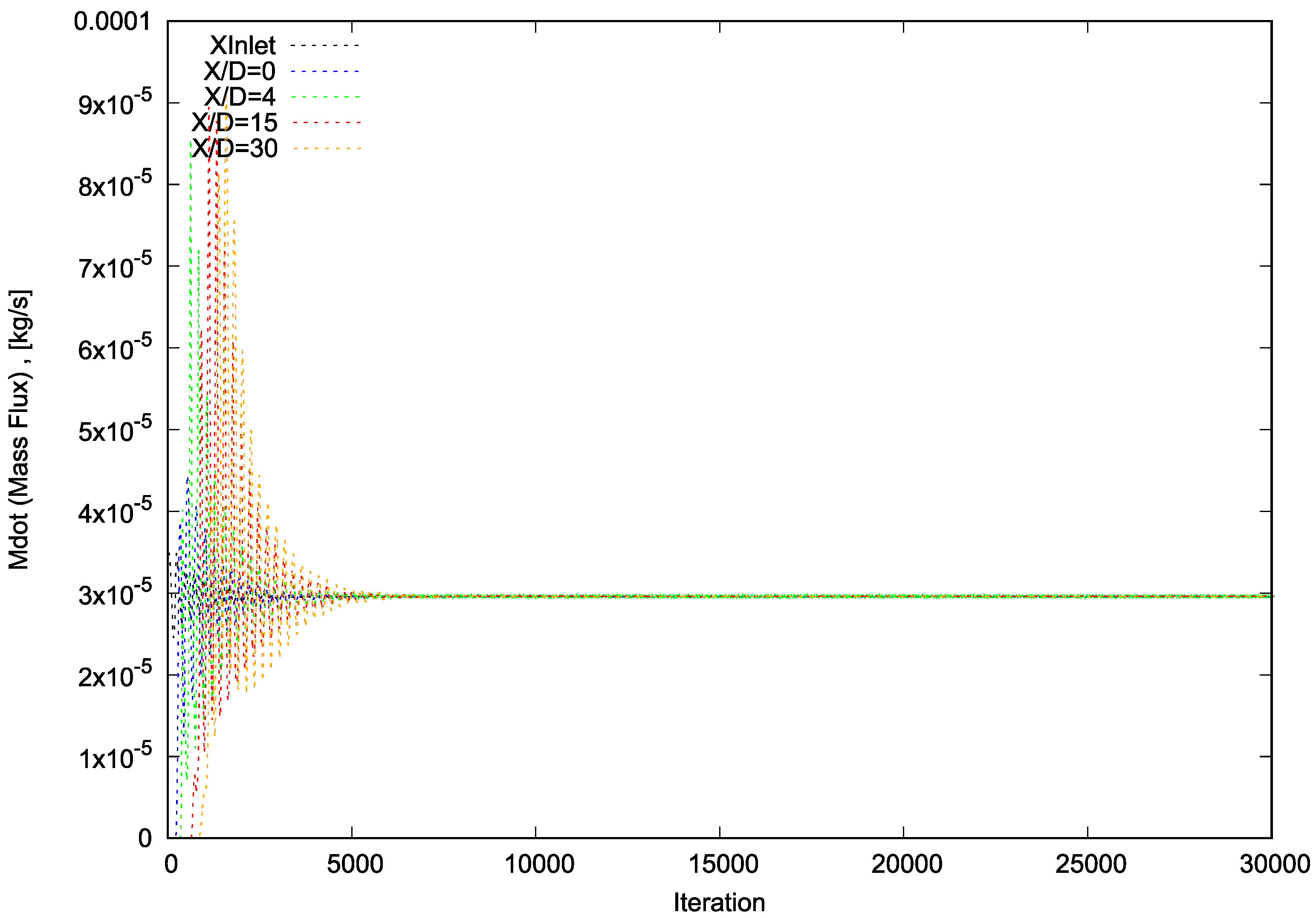
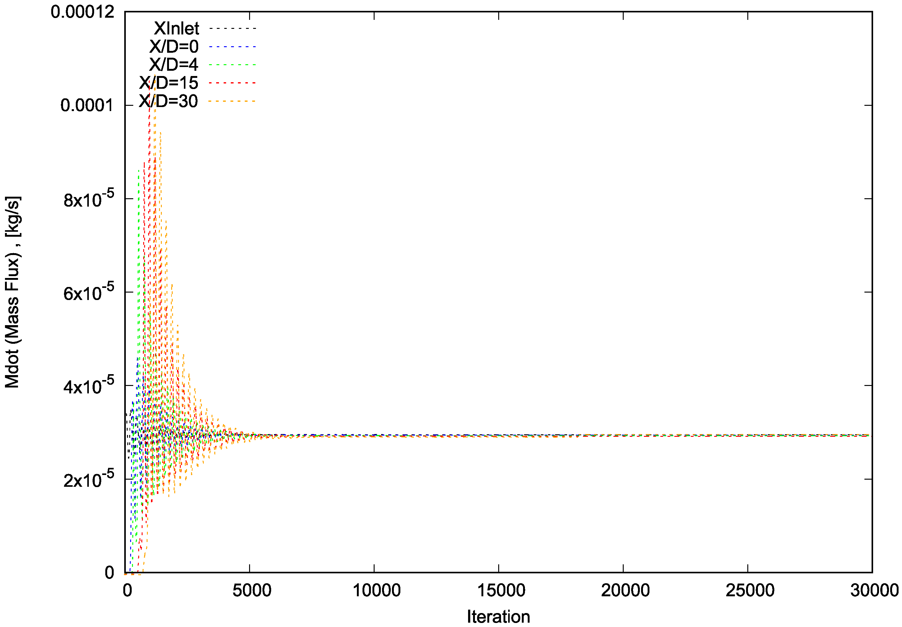
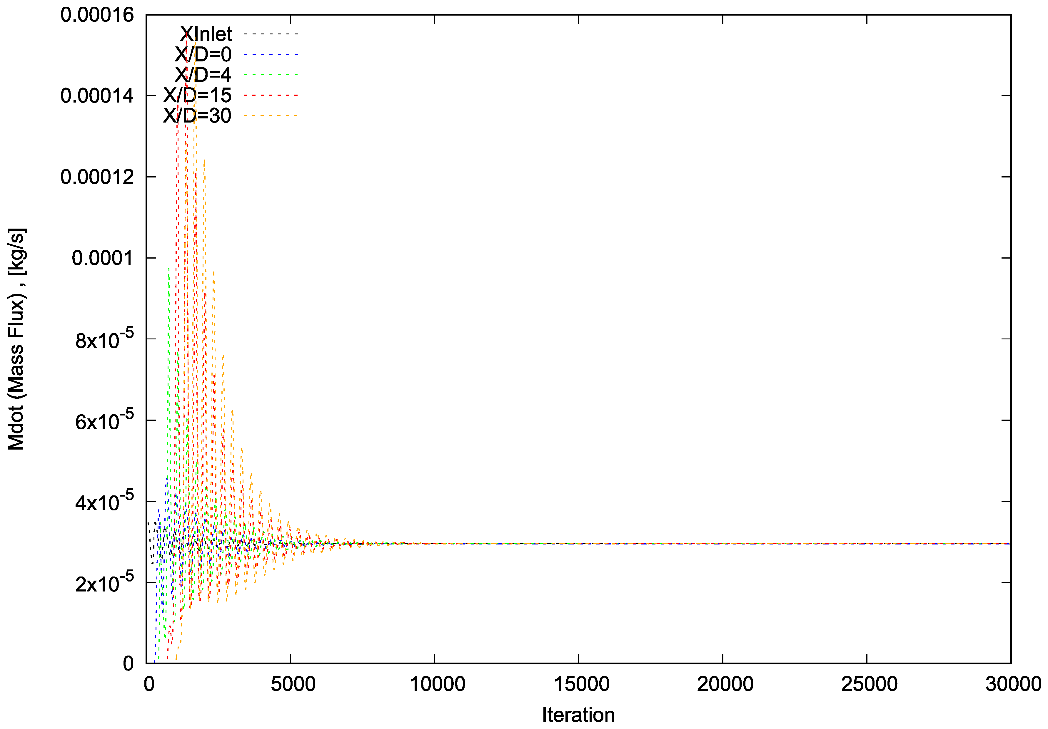
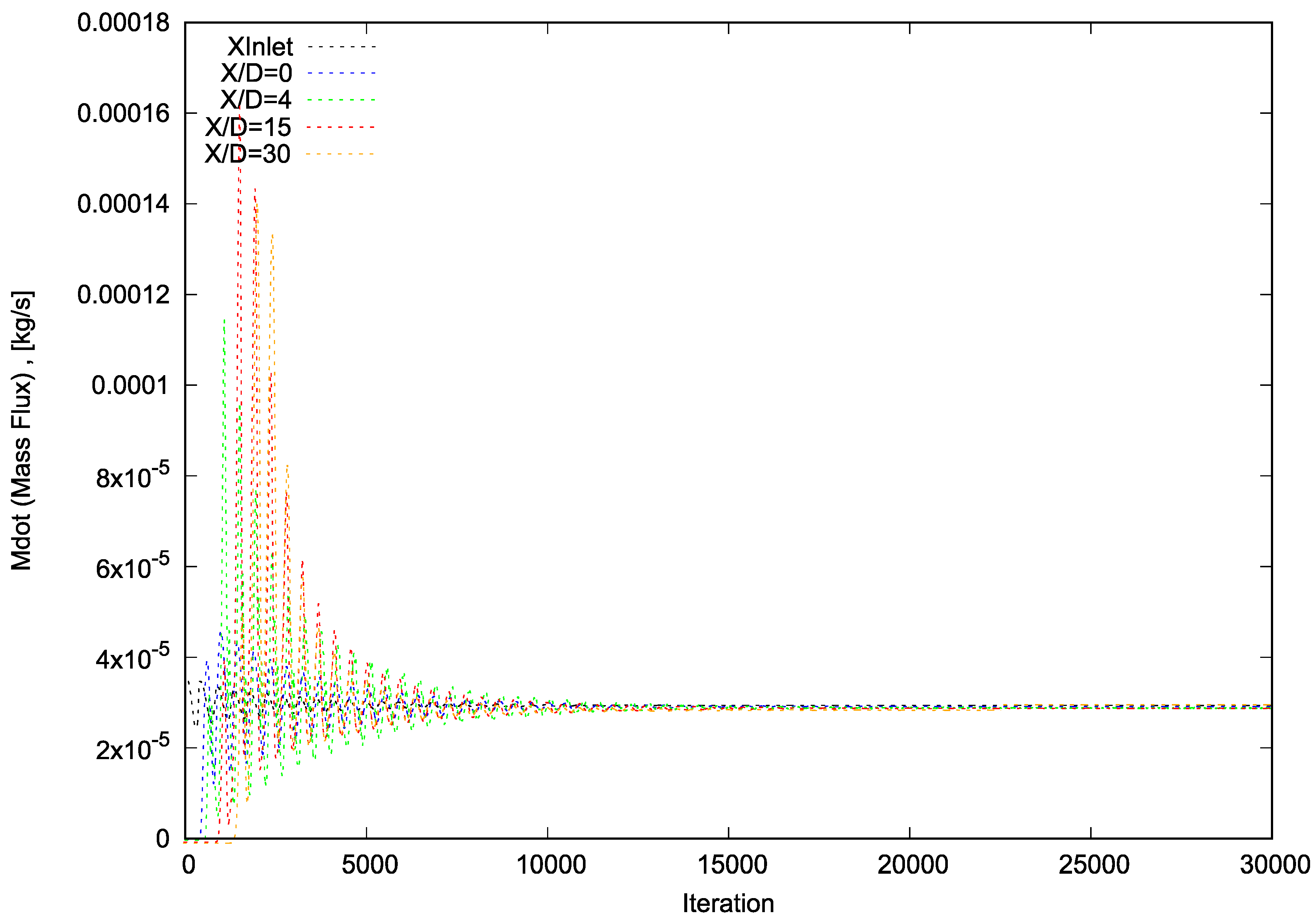
Subsequently, the test cases were executed for 30,000 iterations. The massGraph file was utilized to generate massGraph.eps for every test case, which was then used to analyze the necessary iterations for convergence [
2,
3,
4,
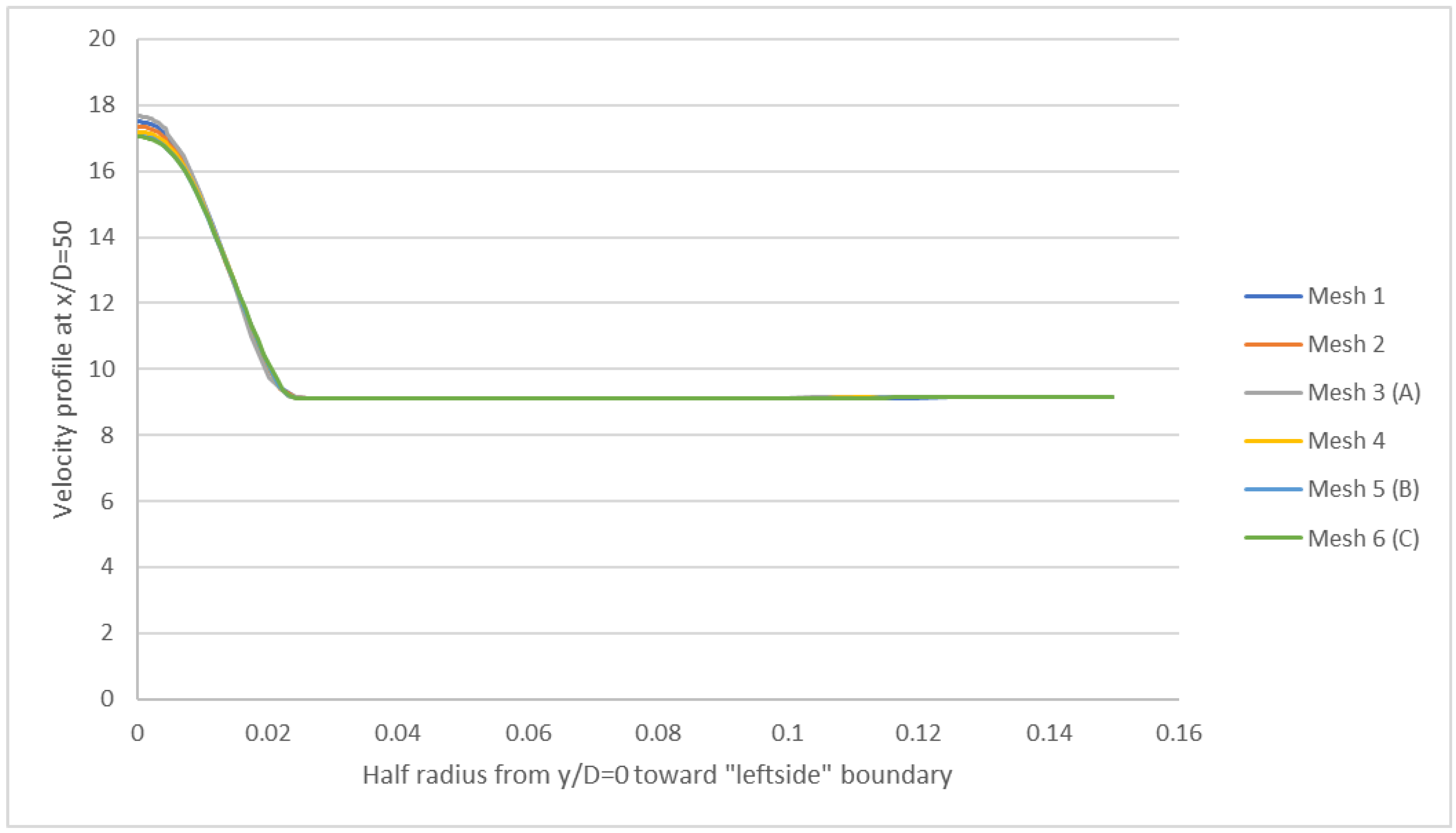
5]. The independent grid was selected by comparing the profile of the half radius of the velocity at x/D = 50 for all test cases (Figure 36). Moreover, the figures of velocity and pressure (p) are demonstrated. The performance phases of each test case were carried out in serial mode (on a single CPU) on a standard personal laptop using the Allrun script file. The precision of numerical measurements was assessed by examining convergence diagrams of mass flux and total momentum for Propane at four reference levels (x/D = 0, 4, 15, and 30) for each of the four test cases. The plots presented depict the convergence, as well as the conservation of Propane and the total momentum of Propane.
Upon completion of the necessary iterations for each test case, the total mass flux of the numerical domain (partitioned into 5-degree sections) at all four reference levels has been observed to converge to 2.952 × 10⁻² g/s (equivalent to 2.125 gr/s for the assumed total reference cylinder). This value represents a 7.6% reduction from the measured mass flux obtained through the flow meter and a 2.8% reduction from the mass flux measured by data extracted through the Rayleigh Scattering System and Laser Doppler Velocimetry.
9. Conclusions
The objective of this study was to perform numerical simulations of velocity and mixture fraction fields in a turbulent non-reaction Propane jet flow. The jet flow was introduced into parallel co-flowing air under isothermal conditions. The objective of the research was to conduct a comparison between the numerical outcomes and experimental data acquired from a prior experimental study in Sandia Laboratory (Sandia National Laboratories, California—P.O. Box 969—Livermore, CA 94551-0969, USA):
http://www.sandia.gov/TNF/DataArch/ProJet.html (accessed on 10 March 2023).
The objective was accomplished by meticulously modifying the reactingFoam solver, which is a standard solver in OpenFOAM, using the swak4Foam utility to eliminate reaction and combustion.
The turbulent flow field on a nearly 2D plane, specifically on a 5-degree sector of the experimental domain, was simulated using a two-equation Realizable k-ε eddy viscosity turbulence model. The aim of this methodology was to enhance comprehension of the flow structure and mixing mechanism in a scenario devoid of chemical interaction and heat transfer. The study compared numerical results to experimental data by analyzing numerical axial and radial profiles of mean velocities, turbulence energy, mean mixture fraction, and mixture fraction half radius (Lf).
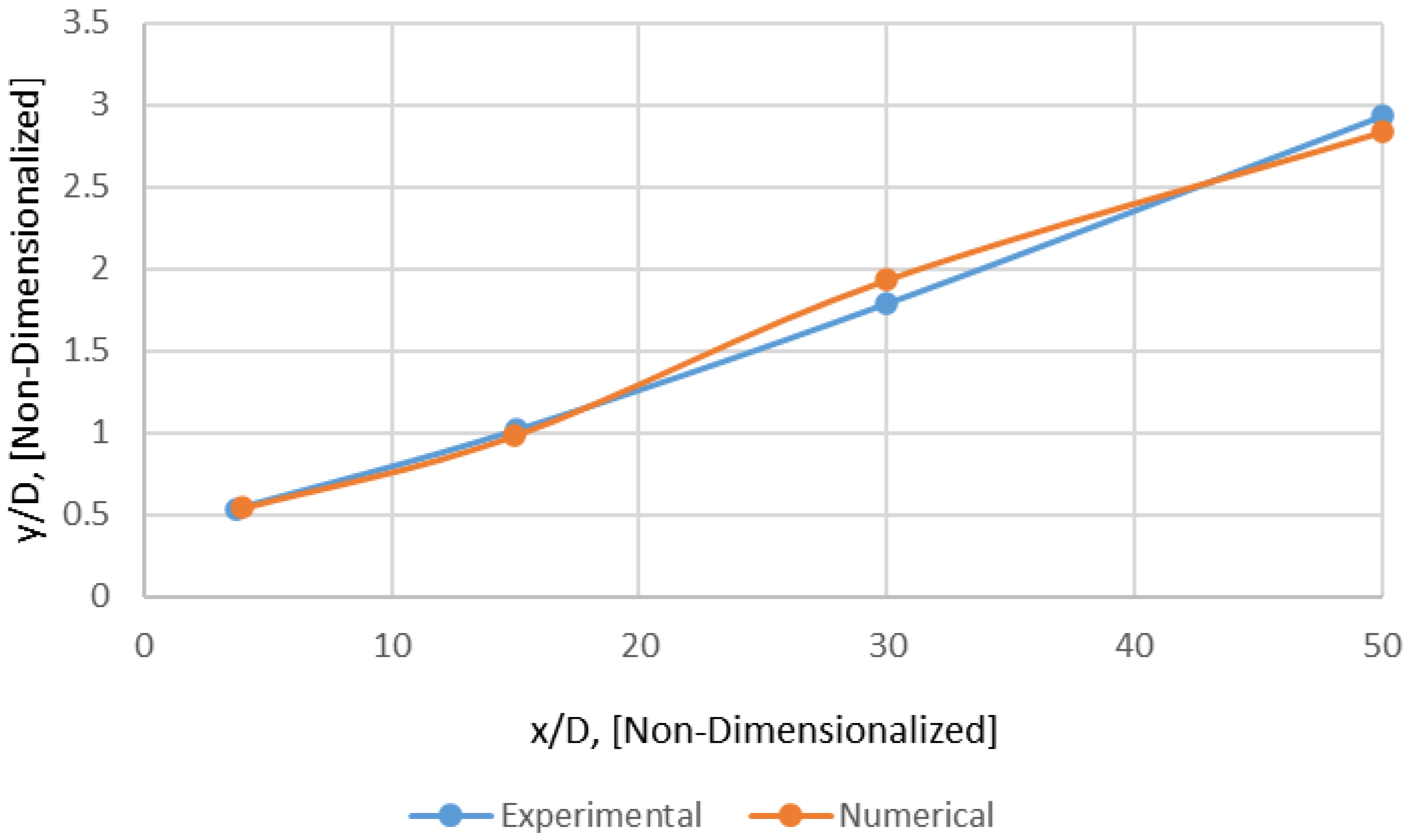
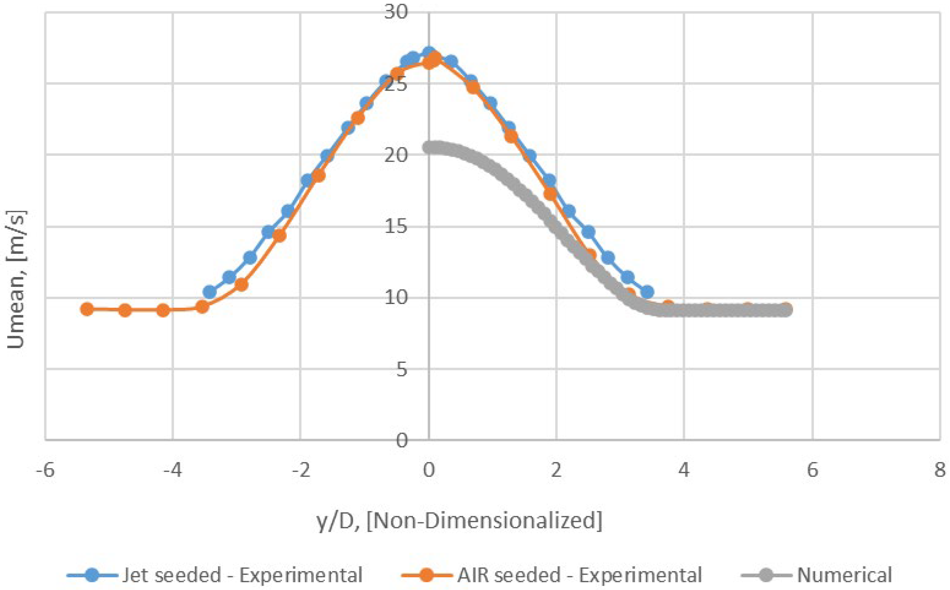
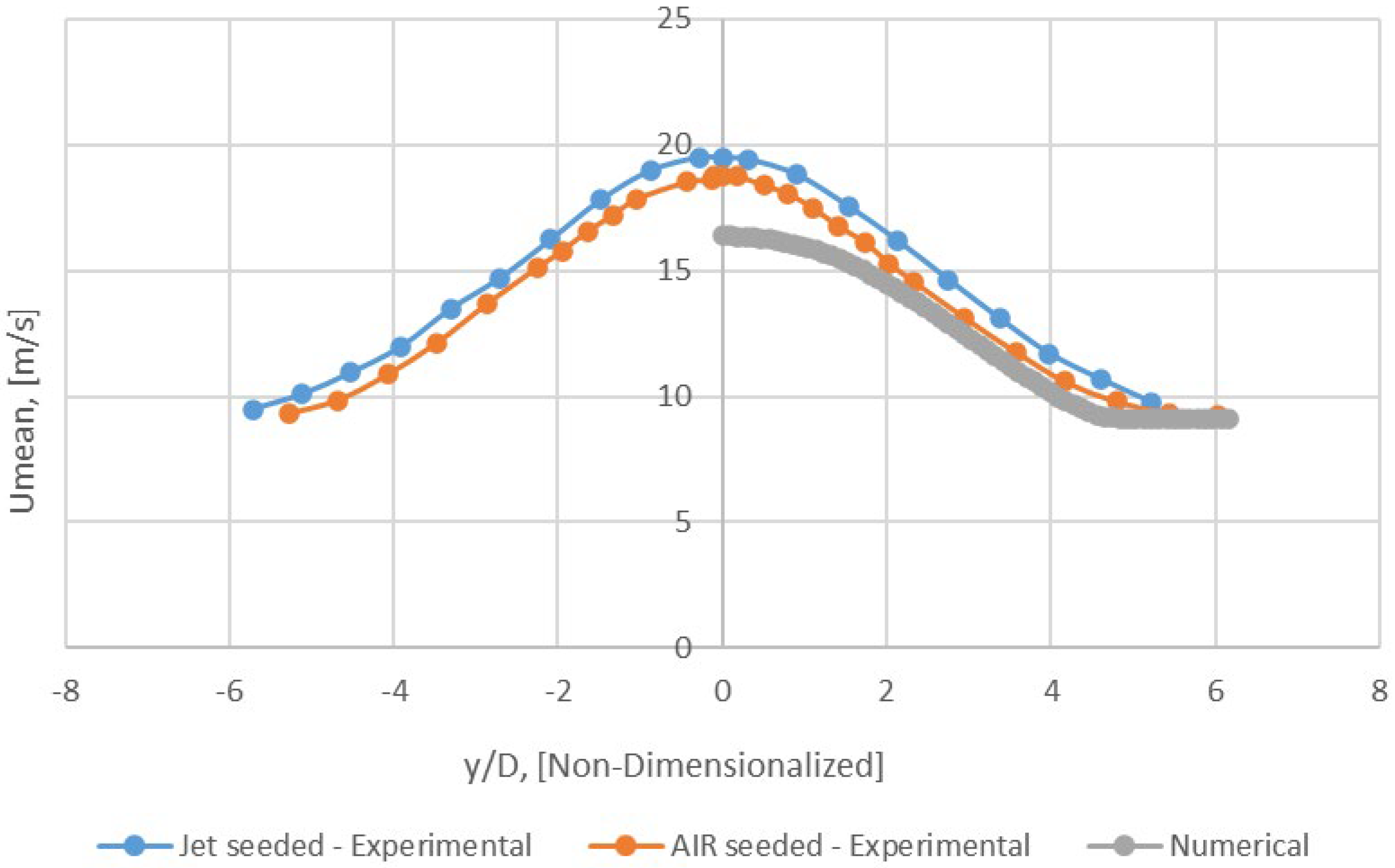
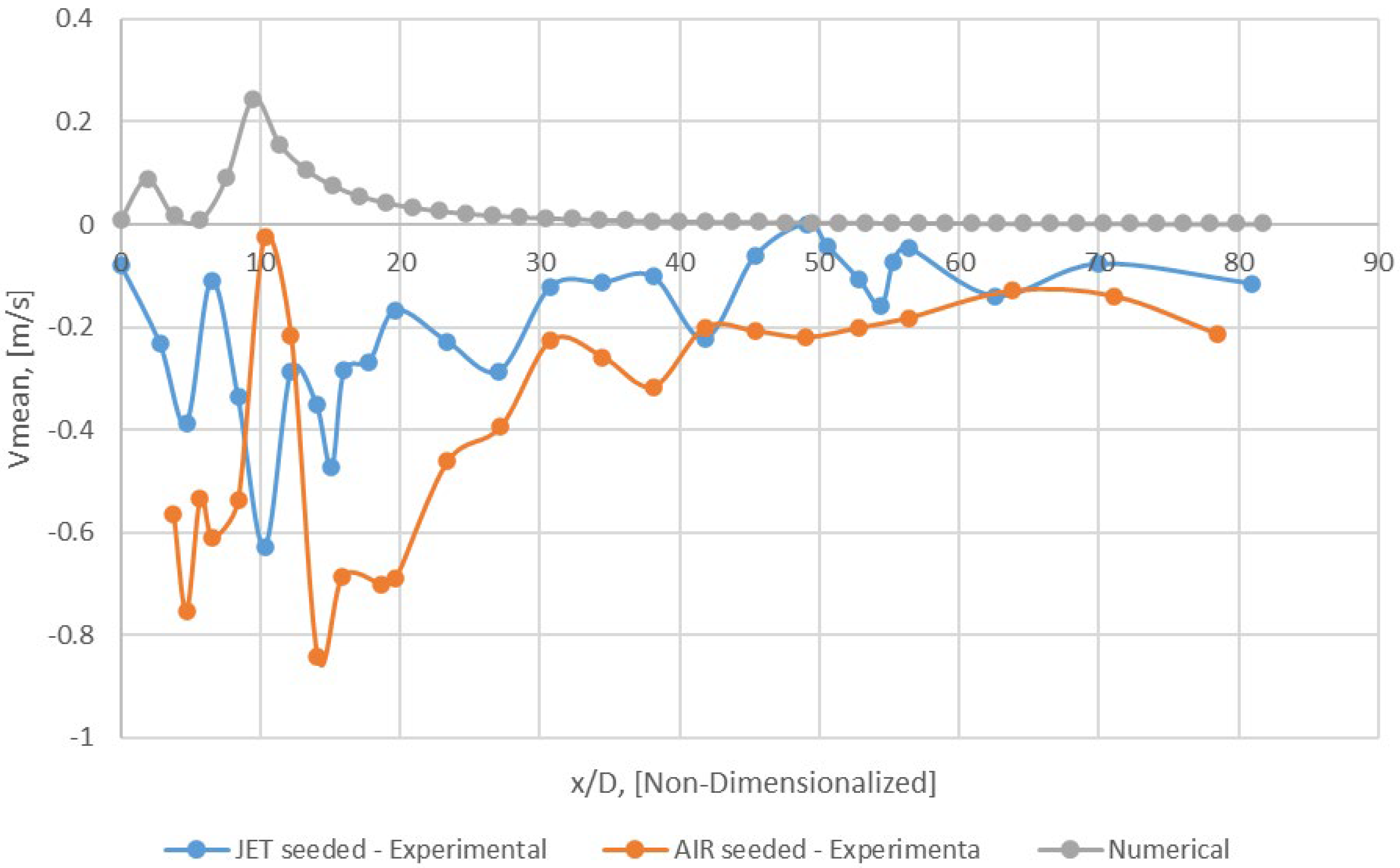
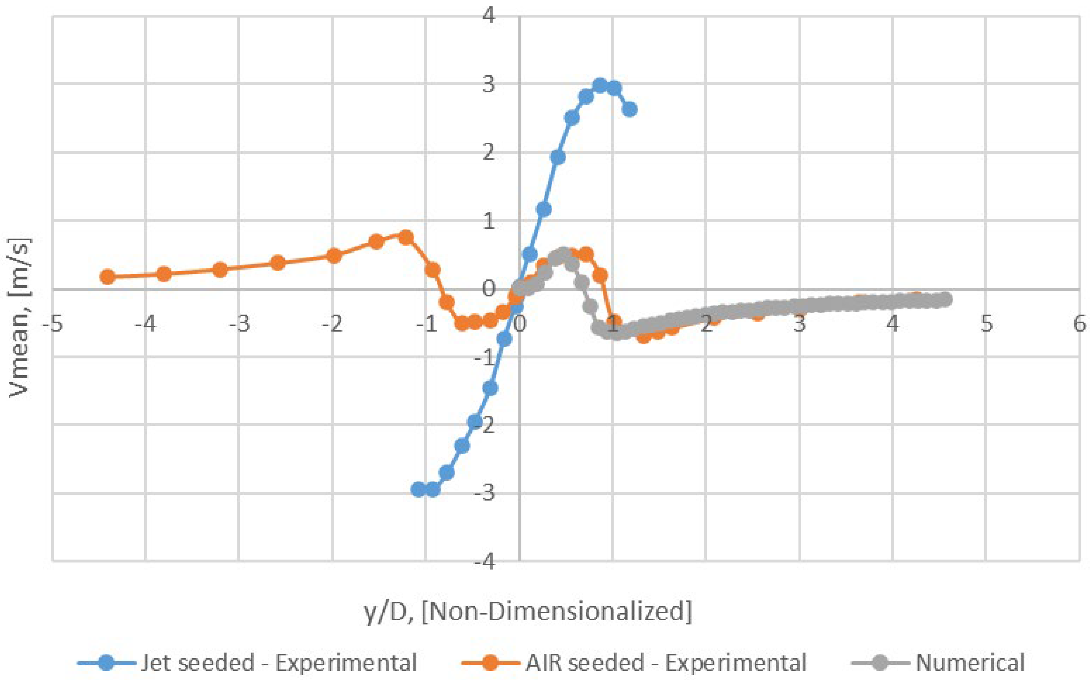
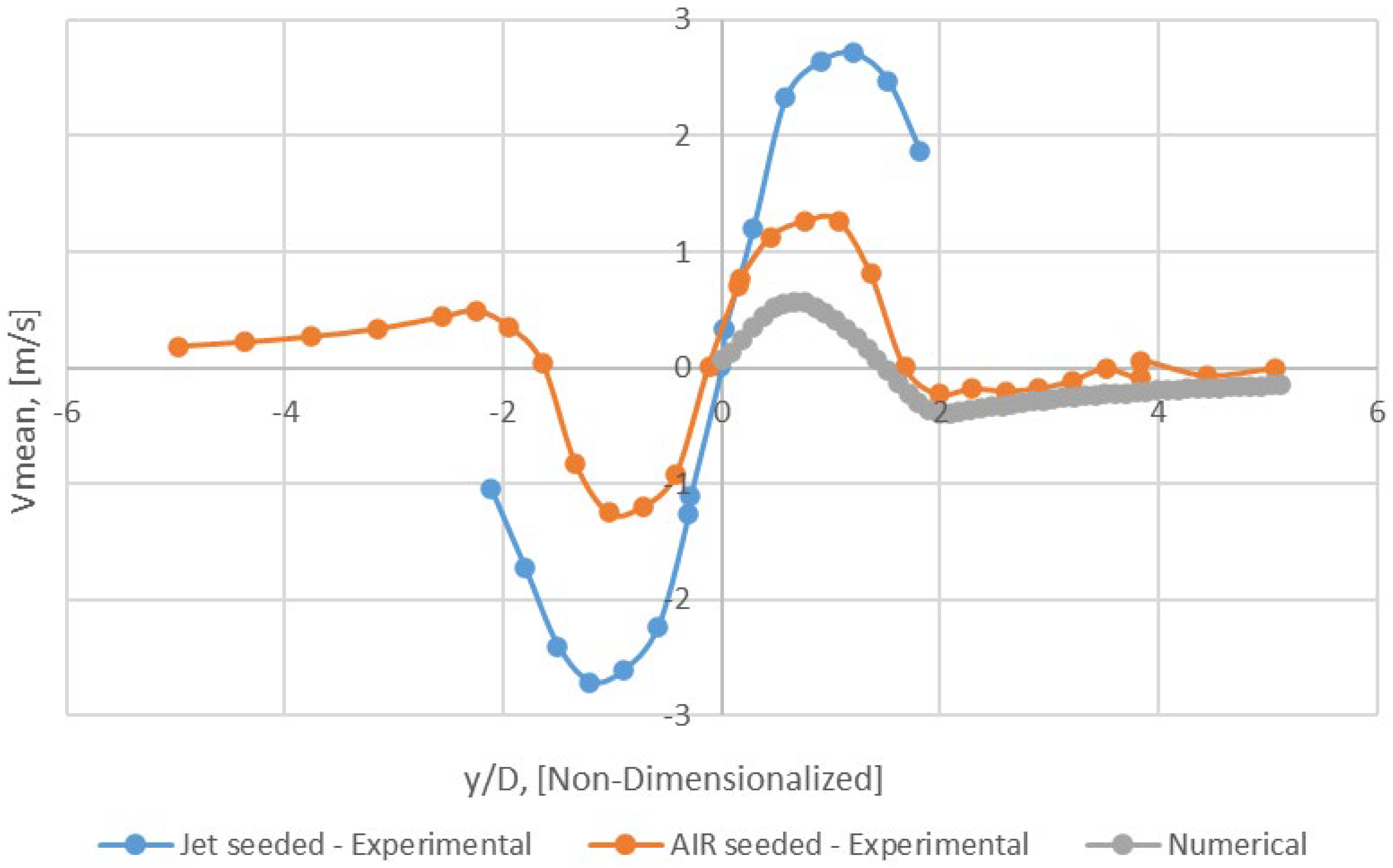
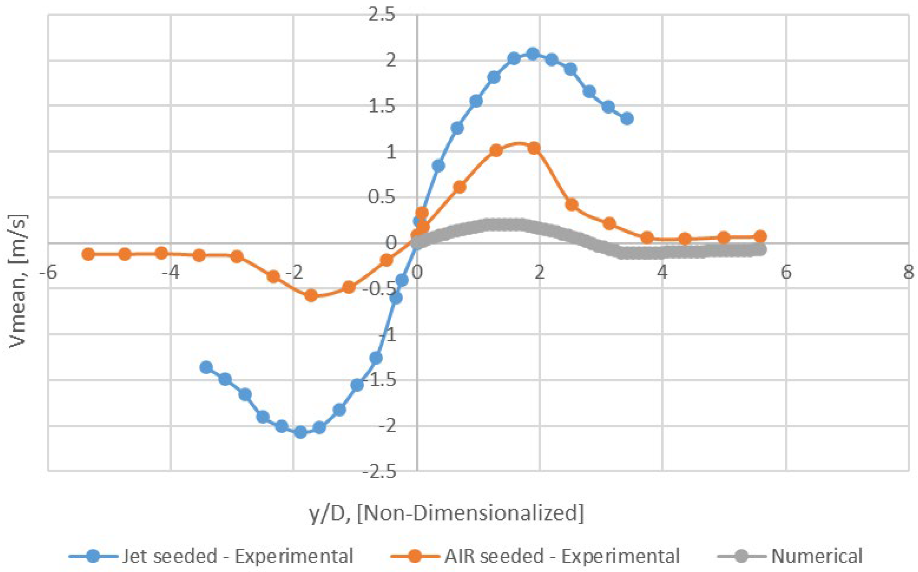
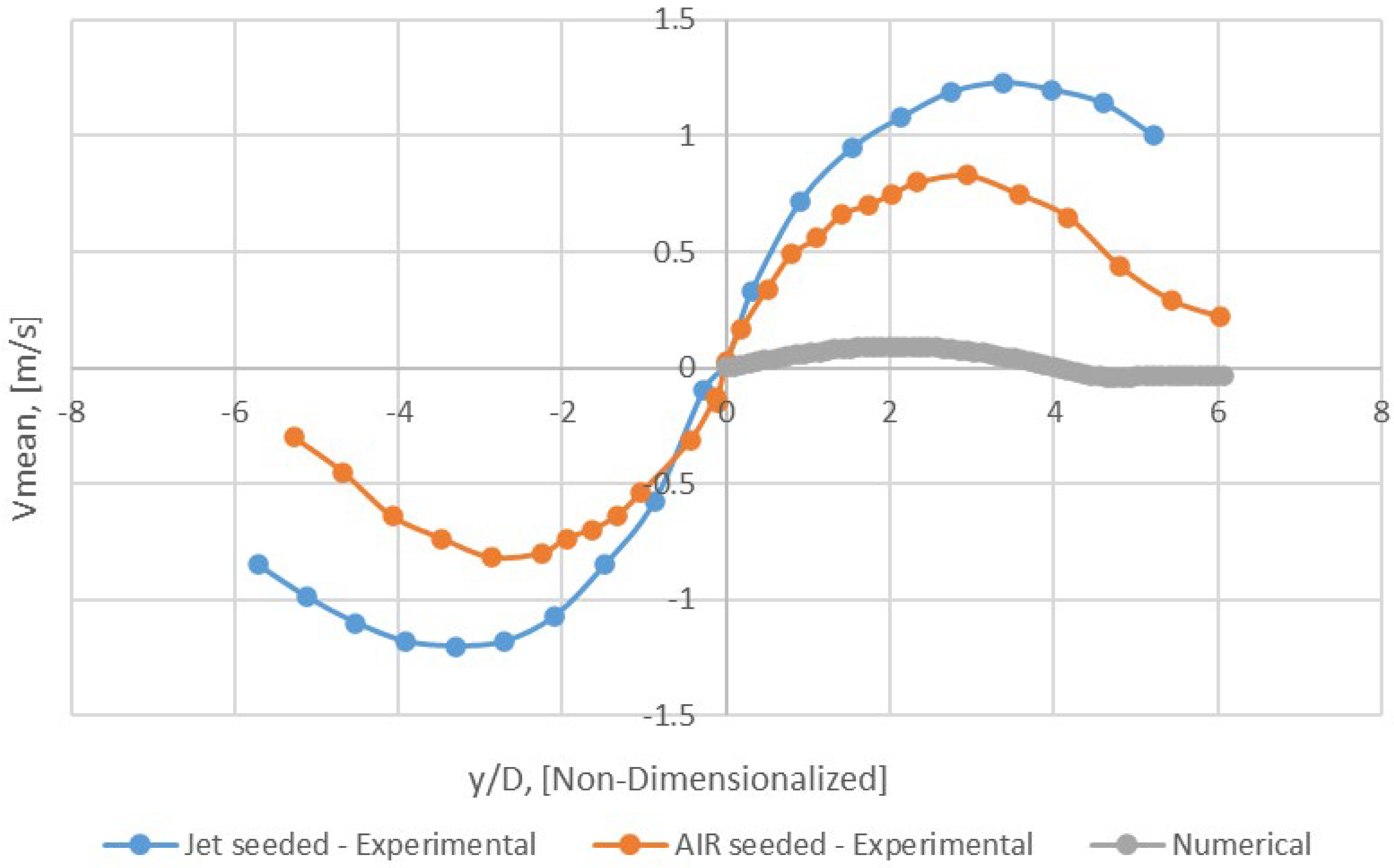
The study demonstrated excellent agreement between the mixture fraction fields and mixture fraction half radius (Lf) obtained from simulations and those obtained from experimental data. Furthermore, it was noted that Umean displayed suitable adjustments, particularly in regions where the examined areas were angled towards the nozzle exit, unlike Vmean. The numerical results showed precise and conforming outcomes with experimental data in the mentioned areas, despite the simplifying assumptions made in various adjustments and turbulence models.
The study emphasizes the efficacy of the two-equation Realizable k-ε eddy viscosity turbulence model in minimizing computational costs when compared with more advanced turbulence models, such as Launder, Reece, and Rodi Full Reynolds Stress Model (LRR), Speziale, Sarkar, and Gatski (SSG), Detached Eddy Simulation (DES), Large Eddy Simulation (LES), Direct Numerical Simulation (DNS) and their diverse variants. This study’s numerical findings indicate that the approach utilized can accurately predict turbulent non-reaction flows with minimal computational expenses.
Figure 2.
Convergence diagram of mass flux for Mesh A.
Figure 2.
Convergence diagram of mass flux for Mesh A.
Figure 3.
Convergence diagram of mass flux for Mesh B.
Figure 3.
Convergence diagram of mass flux for Mesh B.
Figure 4.
Convergence diagram of mass flux for Mesh C.
Figure 4.
Convergence diagram of mass flux for Mesh C.
Figure 5.
Convergence diagram of mass flux for Mesh D.
Figure 5.
Convergence diagram of mass flux for Mesh D.
Figure 6.
Axial Profile of mixture fraction of Propane − y/D = 0 (Mesh B).
Figure 6.
Axial Profile of mixture fraction of Propane − y/D = 0 (Mesh B).
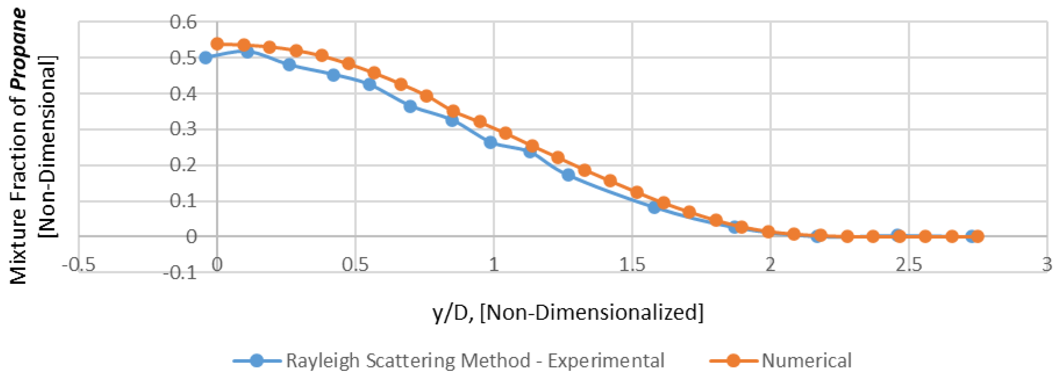
Figure 7.
Radial profile of mixture fraction of Propane − x/D = 4 (Mesh B).
Figure 7.
Radial profile of mixture fraction of Propane − x/D = 4 (Mesh B).
Figure 8.
Radial Profile of mixture fraction of Propane − x/D = 15 (Mesh B).
Figure 8.
Radial Profile of mixture fraction of Propane − x/D = 15 (Mesh B).
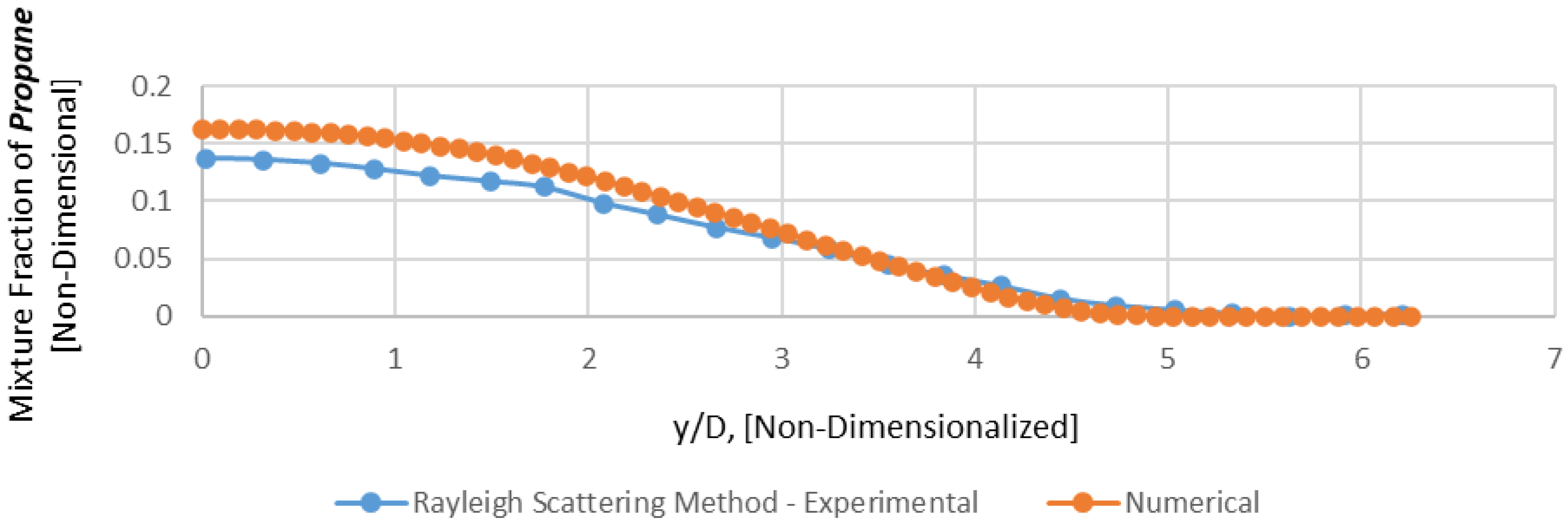
Figure 9.
Radial Profile of mixture fraction of Propane − x/D = 30 (Mesh B).
Figure 9.
Radial Profile of mixture fraction of Propane − x/D = 30 (Mesh B).
Figure 10.
Radial Profile of mixture fraction of Propane − x/D = 50 (Mesh B).
Figure 10.
Radial Profile of mixture fraction of Propane − x/D = 50 (Mesh B).
Figure 11.
Variations of mixture fraction half radius (Lf) with axial distance (Mesh B).
Figure 11.
Variations of mixture fraction half radius (Lf) with axial distance (Mesh B).
Figure 12.
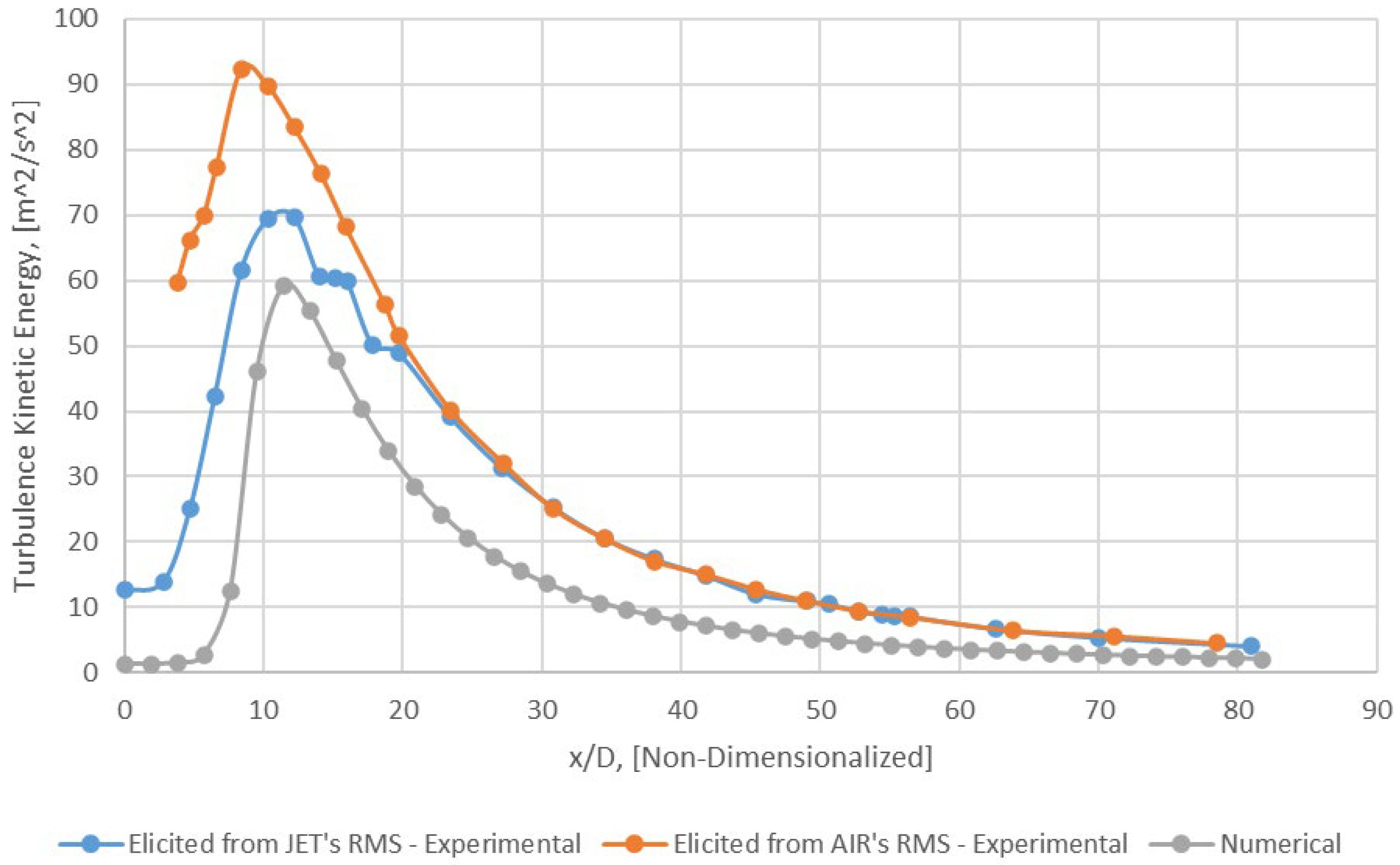
Axial profile of turbulence kinetic energy (k) − y/D = 0 (Mesh B).
Figure 12.
Axial profile of turbulence kinetic energy (k) − y/D = 0 (Mesh B).
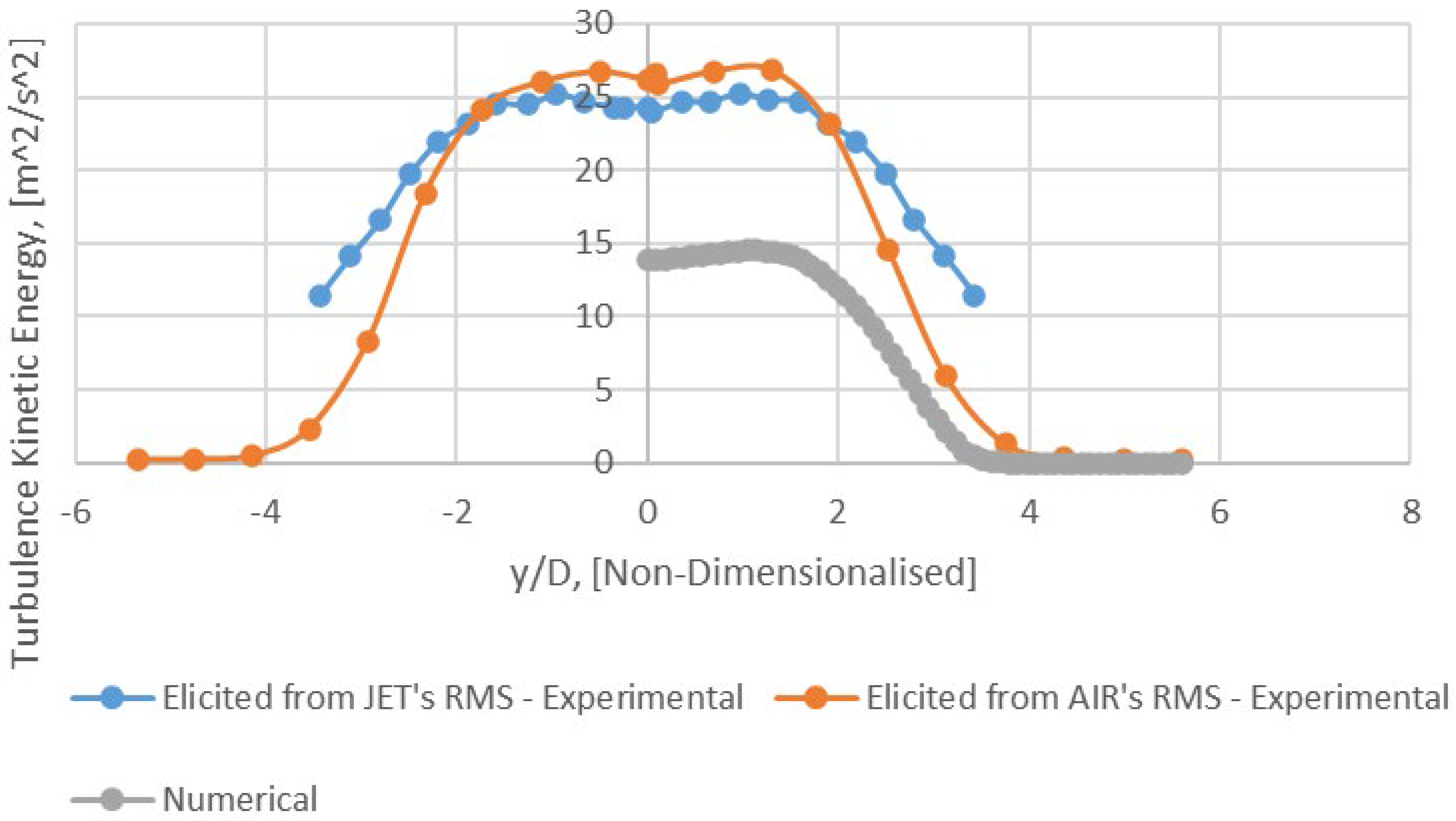
Figure 13.
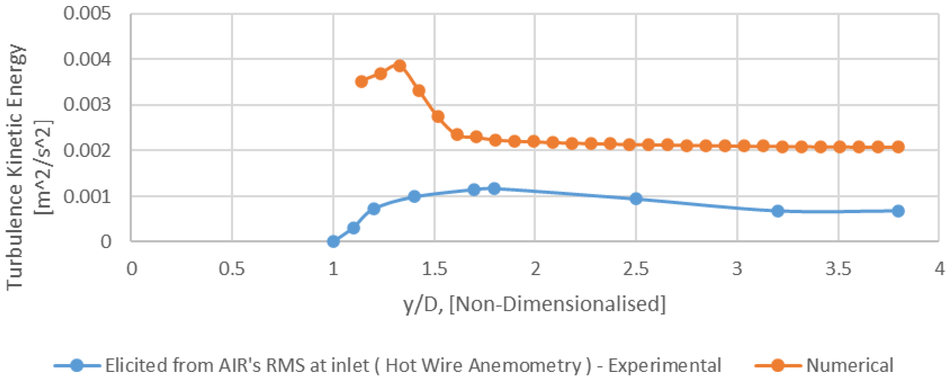
Radial profile of turbulence Kinetic energy (k) for AIR (Hot Wire Anemometry) − x/D = 0 (Mesh B).
Figure 13.
Radial profile of turbulence Kinetic energy (k) for AIR (Hot Wire Anemometry) − x/D = 0 (Mesh B).
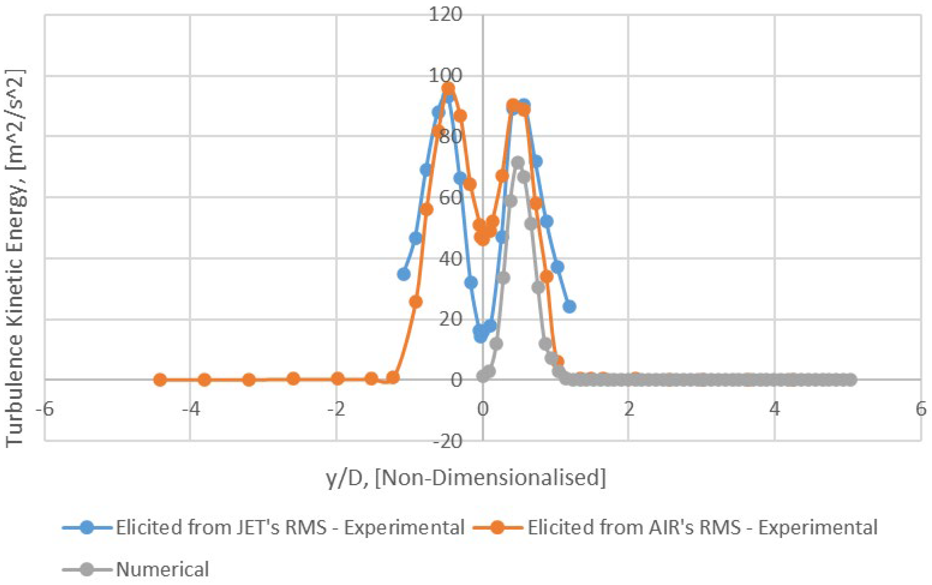
Figure 14.
Radial profile of turbulence kinetic energy (k) − x/D = 4 (Mesh B).
Figure 14.
Radial profile of turbulence kinetic energy (k) − x/D = 4 (Mesh B).
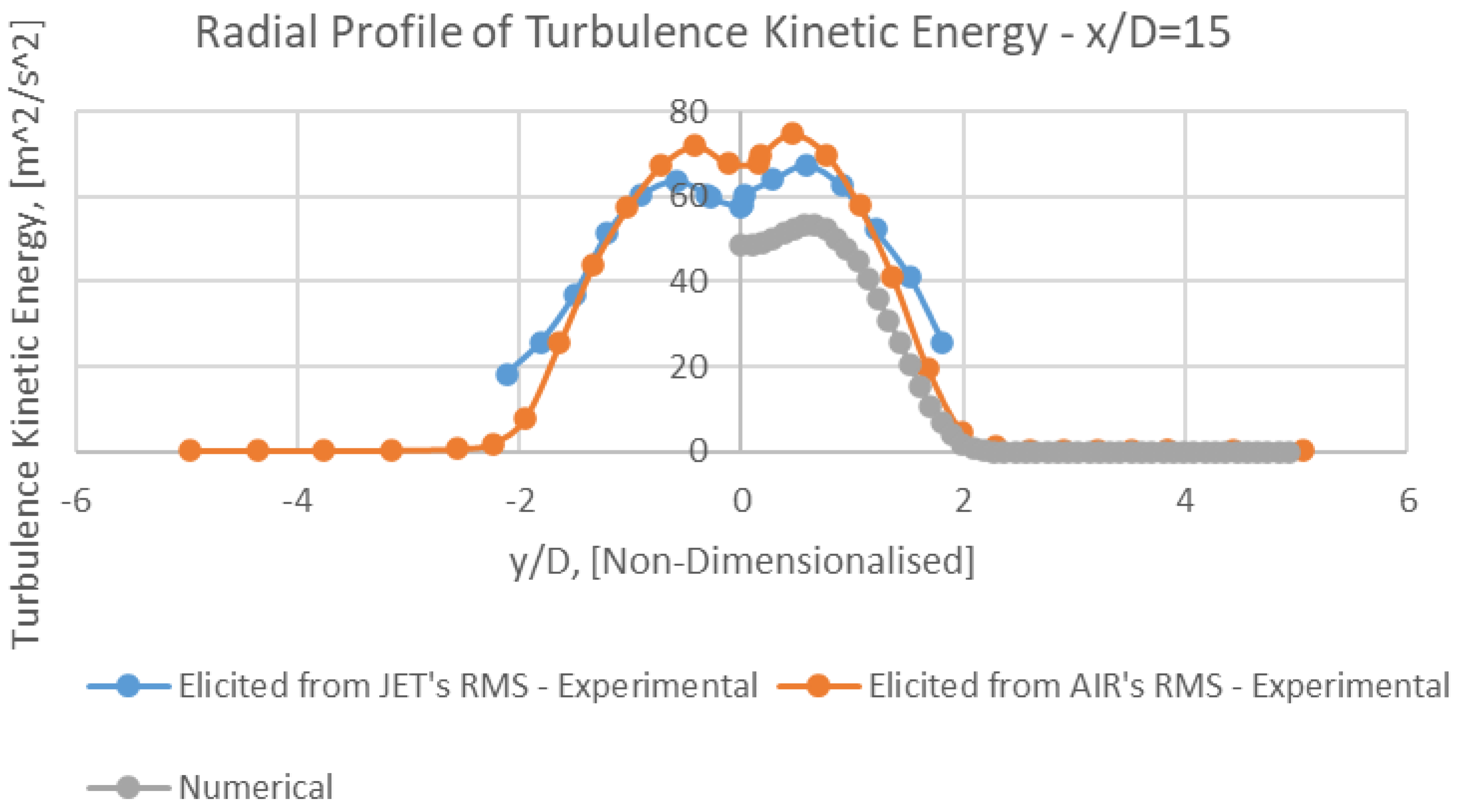
Figure 15.
Radial profile of turbulence kinetic energy (k) − x/D = 15 (Mesh B).
Figure 15.
Radial profile of turbulence kinetic energy (k) − x/D = 15 (Mesh B).
Figure 16.
Radial profile of turbulence kinetic energy (k) − x/D = 30 (Mesh B).
Figure 16.
Radial profile of turbulence kinetic energy (k) − x/D = 30 (Mesh B).
Figure 17.
Radial profile of turbulence kinetic energy (k) − x/D = 50 (Mesh B).
Figure 17.
Radial profile of turbulence kinetic energy (k) − x/D = 50 (Mesh B).
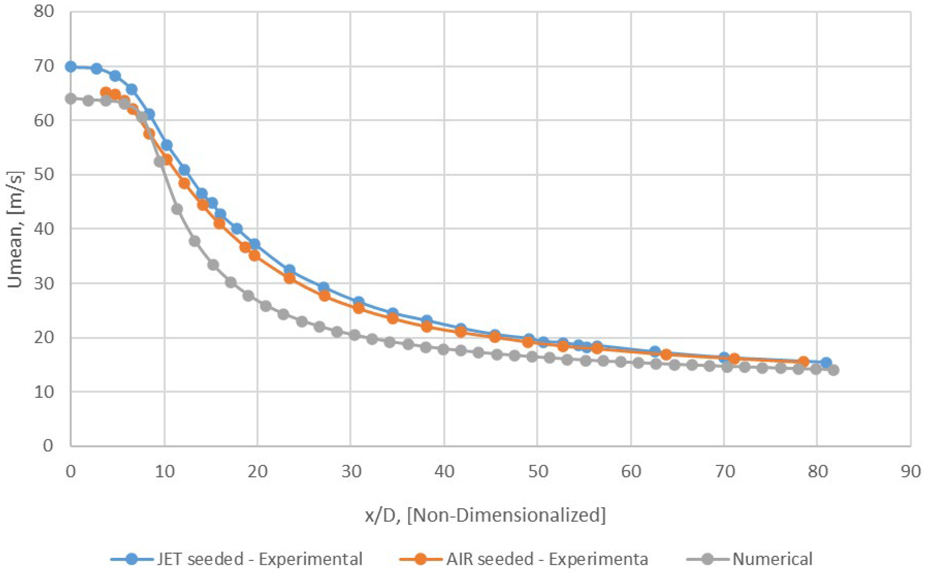
Figure 18.
Axial Profile of Umean − y/D = 0 (Mesh B).
Figure 18.
Axial Profile of Umean − y/D = 0 (Mesh B).
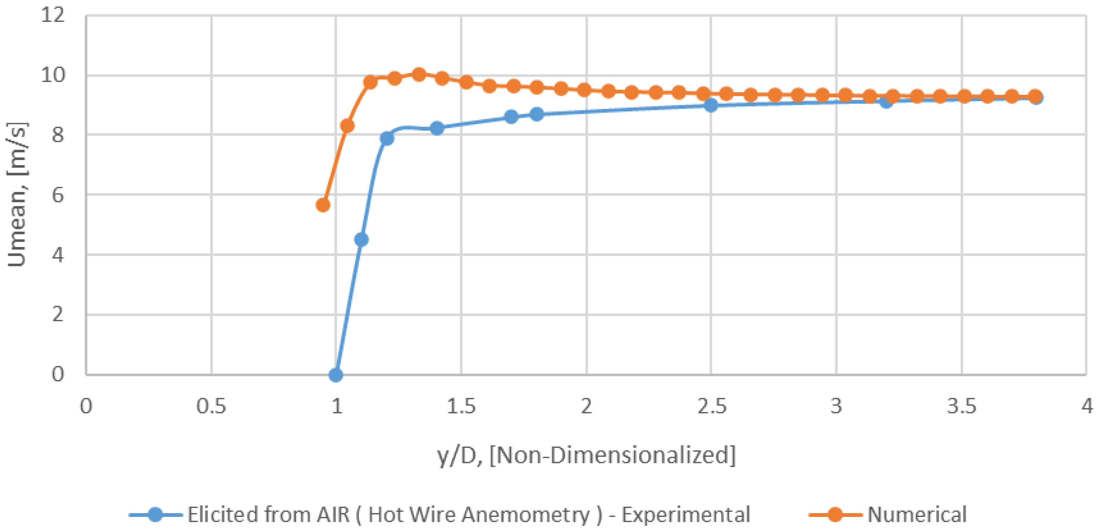
Figure 19.
Radial profile of Umean for AIR (Hot Wire Anemometry) − x/D = 0 (Mesh B).
Figure 19.
Radial profile of Umean for AIR (Hot Wire Anemometry) − x/D = 0 (Mesh B).
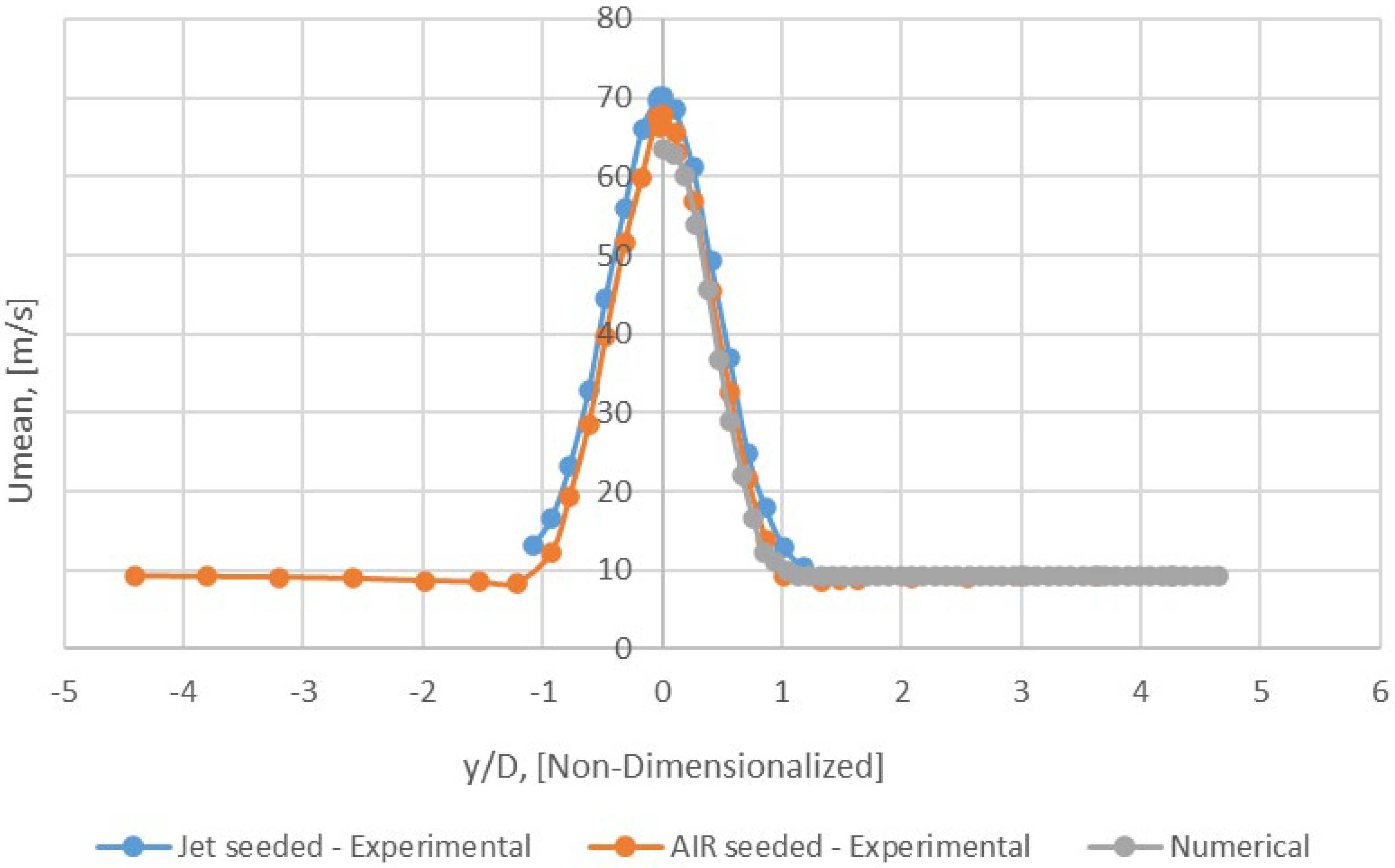
Figure 20.
Radial profile of Umean − x/D = 4 (Mesh B).
Figure 20.
Radial profile of Umean − x/D = 4 (Mesh B).
Figure 21.
Radial profile of Umean − x/D = 15 (Mesh B).
Figure 21.
Radial profile of Umean − x/D = 15 (Mesh B).
Figure 22.
Radial profile of Umean − x/D = 30 (Mesh B).
Figure 22.
Radial profile of Umean − x/D = 30 (Mesh B).
Figure 23.
Radial profile of Umean − x/D = 50 (Mesh B).
Figure 23.
Radial profile of Umean − x/D = 50 (Mesh B).
Figure 24.
Axial profile of Vmean − y/D = 0 (Mesh B).
Figure 24.
Axial profile of Vmean − y/D = 0 (Mesh B).
Figure 25.
Radial profile of Vmean − x/D = 4 (Mesh B).
Figure 25.
Radial profile of Vmean − x/D = 4 (Mesh B).
Figure 26.
Radial profile of Vmean − x/D = 15 (Mesh B).
Figure 26.
Radial profile of Vmean − x/D = 15 (Mesh B).
Figure 27.
Radial profile of Vmean − x/D = 30 (Mesh B).
Figure 27.
Radial profile of Vmean − x/D = 30 (Mesh B).
Figure 28.
Radial profile of Vmean − x/D = 50 (Mesh B).
Figure 28.
Radial profile of Vmean − x/D = 50 (Mesh B).
Figure 29.
Schematic domain B.
Figure 29.
Schematic domain B.
Figure 30.
Schematic of a mesh.
Figure 30.
Schematic of a mesh.
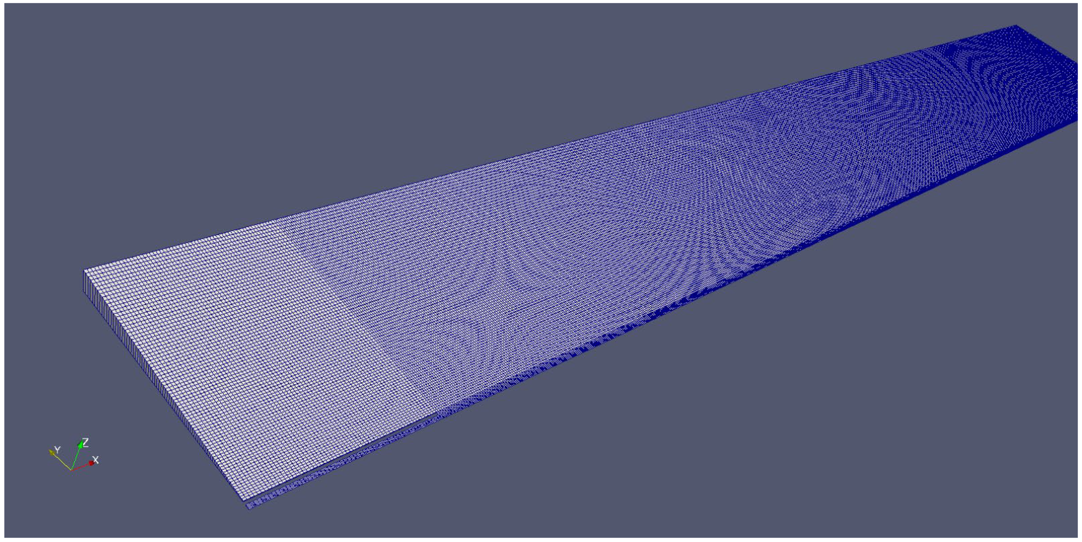
Figure 31.
Schematic of Mesh B.
Figure 31.
Schematic of Mesh B.
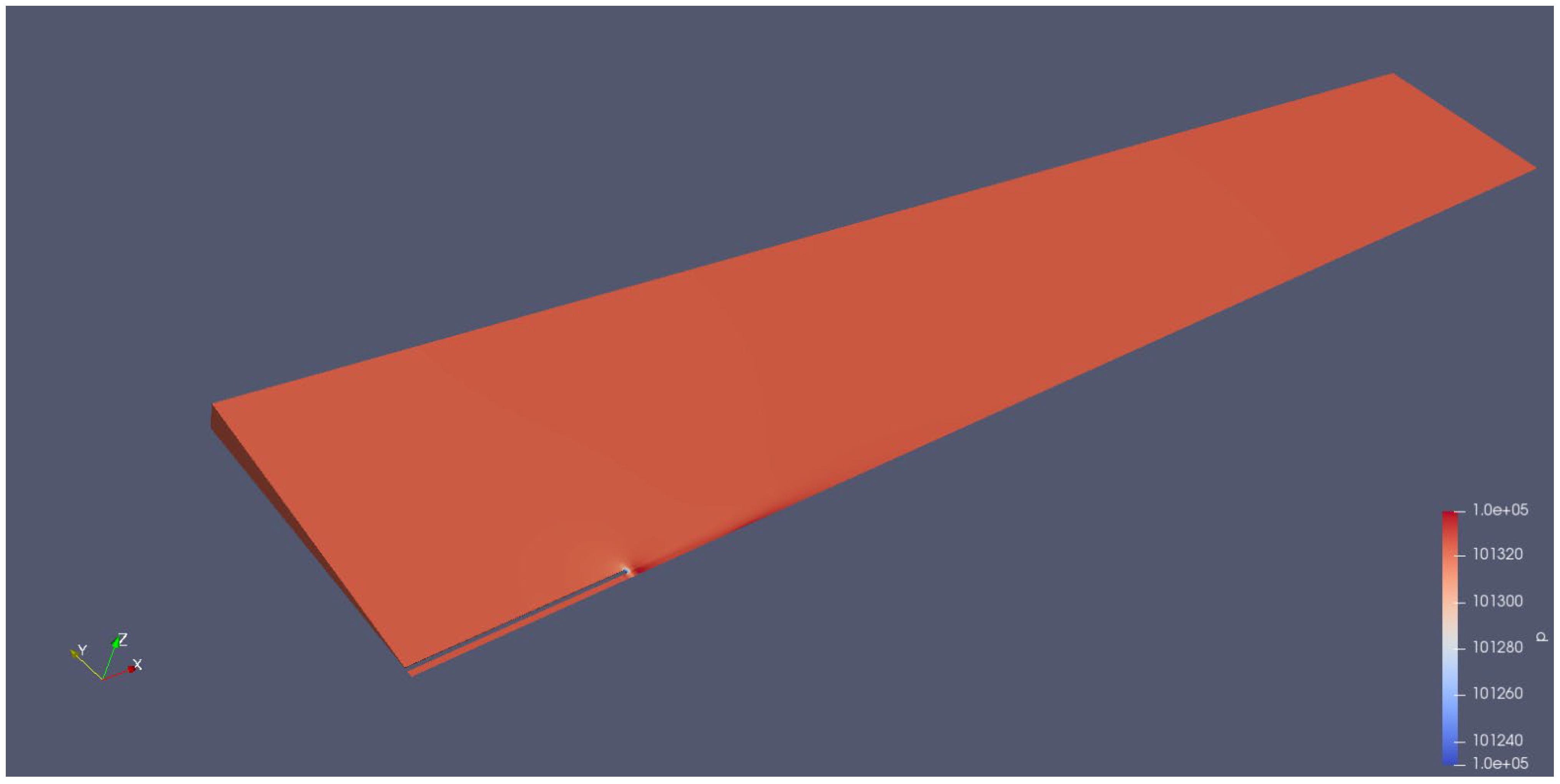
Figure 32.
Pressure (Mesh B).
Figure 32.
Pressure (Mesh B).
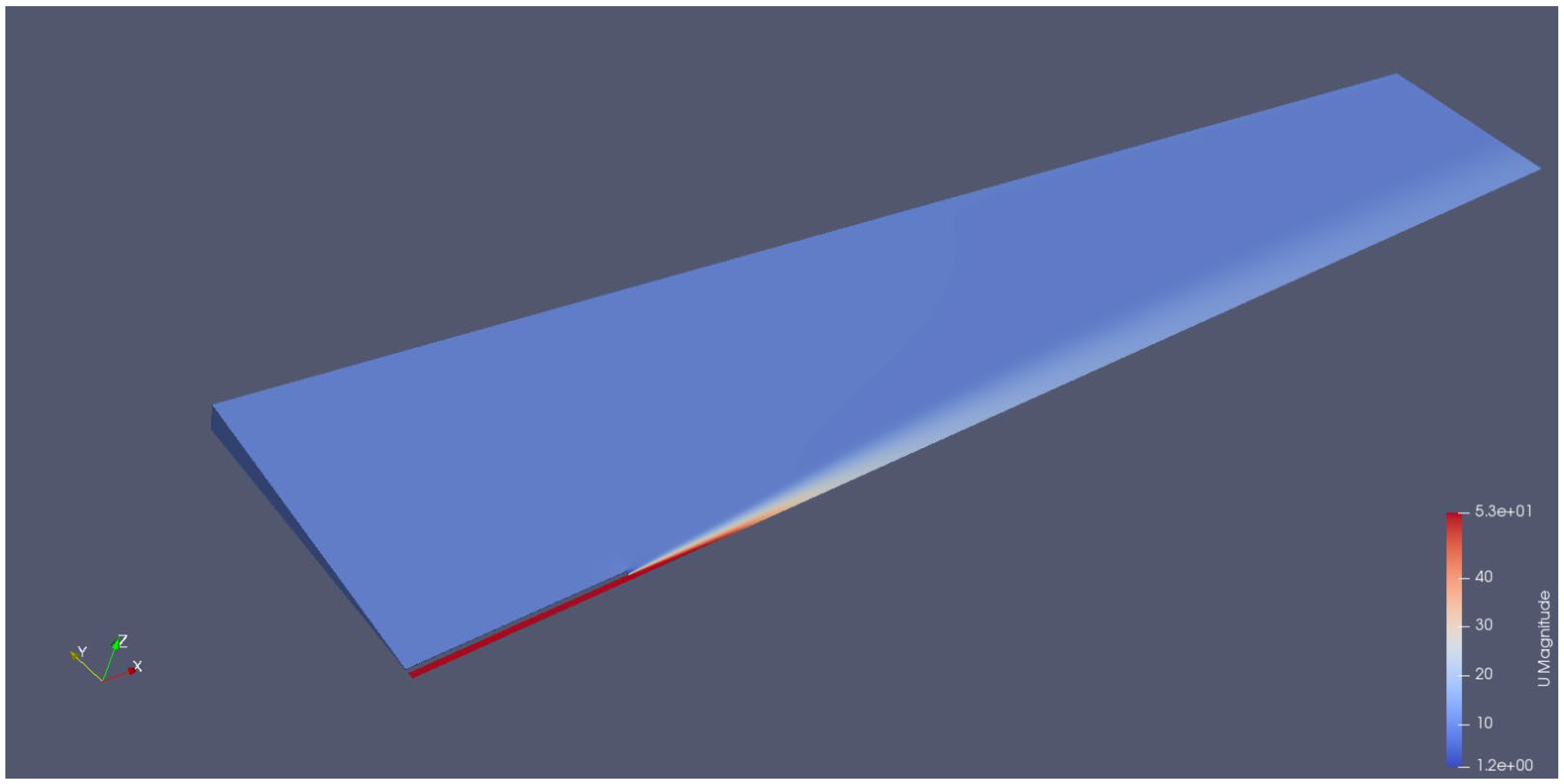
Figure 33.
Velocity (Mesh B).
Figure 33.
Velocity (Mesh B).
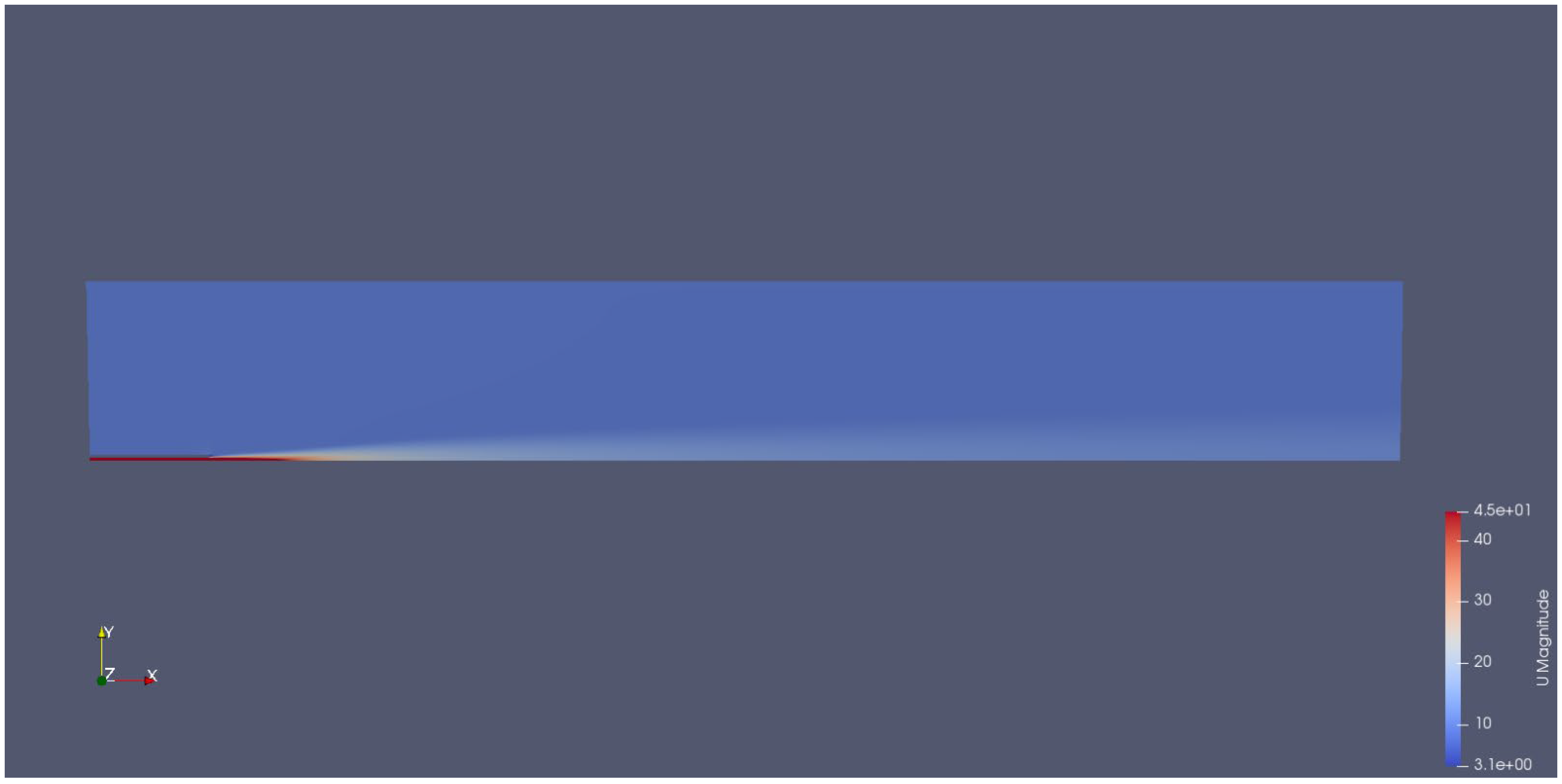
Figure 34.
Velocity (Mesh B).
Figure 34.
Velocity (Mesh B).
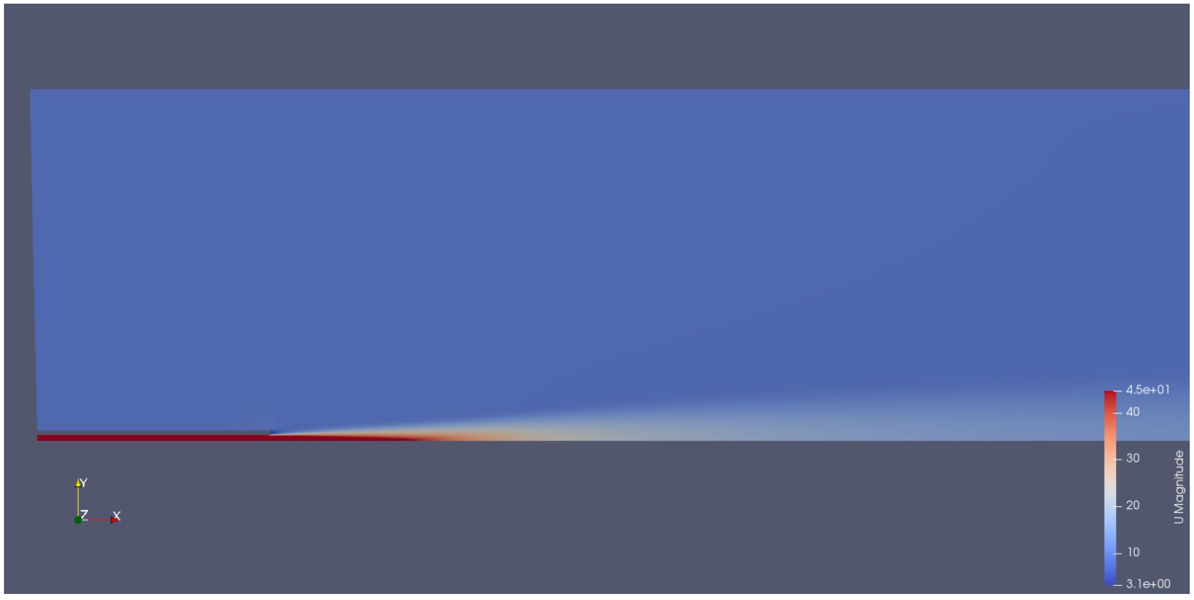
Figure 35.
Velocity (Mesh B).
Figure 35.
Velocity (Mesh B).
Figure 36.
Mesh independency comparison for a half radius of the velocity profile at x/D = 50.
Figure 36.
Mesh independency comparison for a half radius of the velocity profile at x/D = 50.


