Radial Based Approximations for Arcsine, Arccosine, Arctangent and Applications


School of Electrical Engineering, Computing and Mathematical Sciences, Curtin University, Perth 6845, Australia
AppliedMath 2023, 3(2), 343-394; https://doi.org/10.3390/appliedmath3020019
Submission received: 30 September 2022
/
Revised: 12 December 2022
/
Accepted: 15 December 2022
/
Published: 4 April 2023
Abstract
:Based on the geometry of a radial function, a sequence of approximations for arcsine, arccosine and arctangent are detailed. The approximations for arcsine and arccosine are sharp at the points zero and one. Convergence of the approximations is proved and the convergence is significantly better than Taylor series approximations for arguments approaching one. The established approximations can be utilized as the basis for Newton-Raphson iteration and analytical approximations, of modest complexity, and with relative error bounds of the order of , and lower, can be defined. Applications of the approximations include: first, upper and lower bounded functions, of arbitrary accuracy, for arcsine, arccosine and arctangent. Second, approximations with significantly higher accuracy based on the upper or lower bounded approximations. Third, approximations for the square of arcsine with better convergence than well established series for this function. Fourth, approximations to arccosine and arcsine, to even order powers, with relative errors that are significantly lower than published approximations. Fifth, approximations for the inverse tangent integral function and several unknown integrals.
Keywords:
arcsine; arccosine; arctangent; two point spline approximation; upper and lower bounded functions; Newton-RaphsonMSC:
26A09; 26A18; 26D05; 41A151. Introduction
The elementary trigonometric functions are fundamental to many areas of mathematics with, for example, Fourier theory being widely used and finding widespread applications. The formulation of trigonometric results was pre-dated by interest in the geometry of triangles and this occurs well in antiquity, e.g., [1]. The fundamental functions of sine and cosine have a geometric basis and are naturally associated with an angle from the positive horizontal axis to a point on the unit circle. From angle addition and difference identities for sine and cosine, the derivatives of these functions can be defined and, subsequently, Taylor series approximations for sine and cosine can be established. Such approximations have reasonable convergence with a ninth order expansion having a relative error bound of for the interval . Naturally, many other approximations have been developed, e.g., [2,3,4].
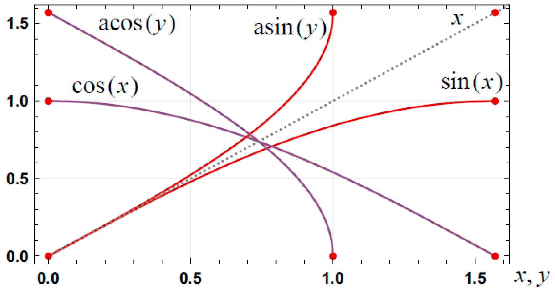
The inverse trigonometric functions of arcsine, arccosine and arctangent are naturally of interest and find widespread use for both the general complex case and the real case. The arctangent function, for example, is found in the solution of the sine-Gordon partial differential equation for the case of soliton wave propagation, e.g., [5]. In statistical analysis the arcsine distribution is widely used and the arctangent function is the basis of a wide class of distributions, e.g., [6]. The graphs of sine, cosine, arcsine and arccosine are shown in Figure 1.
Taylor series expansions for arcsine and arccosine, unlike those for sine and cosine, have relatively poor convergence properties over the interval and a potential problem with respect to finding approximations is that both arcsine and arccosine have undefined derivatives at the point one. An overview of established approximations for arcsine and arctangent is provided in Section 2. In this paper, a geometric approach based on a radial function, whose derivatives are well defined at the point one, is used to establish new approximations for arccosine, arcsine and arctangent. The approximations for arccosine and arcsine are sharp (zero relative error) at the points zero and one and have a defined relative error bound over the interval . Convergence of the approximations is proved and the convergence is significantly better, for arguments approaching one, than Taylor series approximations. The established approximations can be utilized as the basis for Newton-Raphson iteration and analytical approximations, of modest complexity, and with relative error bounds of the order of , and lower, can be defined.
Applications for the established approximations are detailed and these include: First, approximations for arcsine, arccosine and arctangent to achieve a set relative error bound. Second, upper and lower bounded approximations, of arbitrary accuracy, for arcsine, arccosine and arctangent. Third, approximations to arccosine and arcsine, of even order powers, which have significantly lower relative error bounds than published approximations. Fourth, approximations for the inverse tangent integral function with significantly lower relative error bounds, over the interval , than established Taylor series based approximations. Fifth, examples of approximations for unknown integrals.
1.1. Fundamental Relationships
For the real case the following relationships hold:
Thus, it is sufficient to detail approximations over the interval for arcsine and arccosine and approximations over the positive real line for arctangent.
Fundamental relationships for arcsine, arccosine and arctangent, e.g., [7] (1.623, 1.624, p. 57) are:
These relationships imply, for example, that approximations for arcsine and arctangent follow from an approximation to arccosine and approximations for arcsine and arccosine follow from an approximation to arctangent.
1.2. Notation
For an arbitrary function , defined over the interval , an approximating function has a relative error, at a point , defined according to . The relative error bound for the approximating function, over the interval , is defined according to
The notation is used for the derivative of a function. In equations, arcsine, arccosine and arctangent are abbreviated, respectively, as asin, acos and atan.
Mathematica has been used to facilitate analysis and to obtain numerical results. In general, the relative error results associated with approximations to arcsine, arccosine and arctangent have been obtained by sampling specified intervals, in either a linear or logarithmic manner, as appropriate, with points.
1.3. Paper Structure
A review of published approximations for arcsine and arctangent is provided in Section 2. In Section 3, the geometry, and analysis, of the radial function that underpins the proposed approximations for arccosine, arcsine and arctangent, is detailed. In Section 4, convergence of the approximations is detailed. In Section 5, the antisymmetric nature of the arctangent function is utilized to establish spline based approximations for this function. In Section 6, iteration, based on the proposed approximations, is utilized to detail approximations with quadratic convergence. Applications of the proposed approximations are detailed in Section 7 and conclusions are stated in Section 8.
2. Published Approximations for Arcsine and Arctangent
The Taylor series expansions for arcsine and arctangent, respectively, are, e.g., [8] (eqns. 4.24.1, 4.24.3, 4.24.4, p. 121)
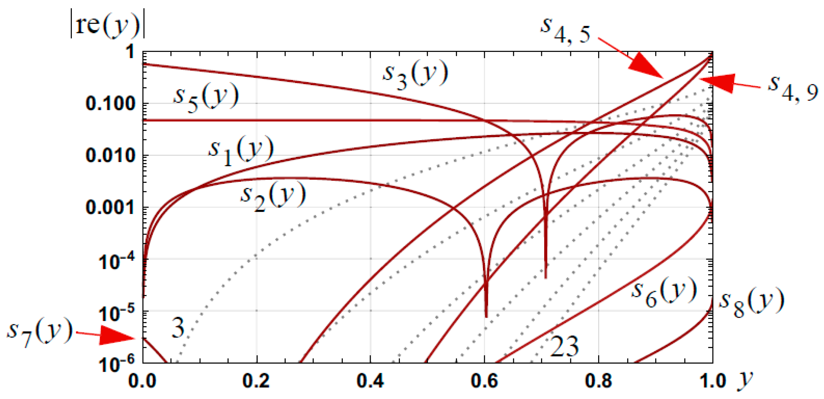
For a set order, the relative error in a Taylor series approximation for arcsine increases sharply as (see Figure 2).
2.1. Approximation Form for Arcsine
The nature of arcsine is such that it has a rate of change of at the origin and an infinite rate of change at the point one which complicates finding suitable approximations. An approximation form that has potential is , whose rate of change is , with the rate of change being at the origin. As a starting point, consider the approximation form
The three coefficients can be chosen to satisfy the constraints consistent with a sharp approximation at the points zero and one: , , and . The constraints imply , , with being arbitrary. For the case of , the approximation is
which has a relative error bound, for the interval , of 2.66 × 10⁻².
2.1.1. Optimized Coefficients
The coefficient can be optimized consistent with minimizing the relative error bound over the interval . The optimum coefficient of leads to the approximation
which has a relative error bound, for the interval [0, 1], of 3.62 × 10⁻³.
2.1.2. Padè Approximants
Given a suitable approximation form, Padè approximants can be utilized to find approximations with lower relative error bounds. For example, the form , where is an approximant of order , can be utilized.
2.2. Published Approximations
The arcsine case is considered as related approximations for arccosine and arctangent follow from Equations (2) and (4). The following approximations are indicative of published approximations. First, the approximation
arises from the simple approximation for arctangent, e.g., [9] (eqn. 5), of
The maximum error in this approximation has a magnitude of 0.0711, but the relative error bound is 0.571, which occurs as approaches zero.
Second, a Taylor series expansion for , e.g., [10] (eqn. 4) or , e.g. [11], can be used. The latter yields the order approximation:
Consistent with a Taylor series, the relative error is low for but, for a set order, becomes increasingly large as .
Third, the following approximations are stated in [12] (eqns. 1.5 and 3.7):
The first approximation is part of the Shafer-Fink inequality (e.g., [13]) is not sharp at the origin and has a relative error bound, for the interval , of 4.72 × 10⁻². The second approximation is not sharp at but has a relative error bound for the interval , of 1.38 × 10⁻³.
Fourth, the following approximation is detailed in [14] (eqn. 4.4.46, p. 81):
where
The relative error bound is 3.04 × 10⁻⁶ which occurs at the origin.
Fifth, [15] (Section 6.4), provides a basis for determining approximations for arcsine, arccosine and arctangent of arbitrary accuracy. Explicit formulas and results are detailed in Appendix A. For example, the following approximation for arcsine (as defined by —see Equation (A13)) is
and has a relative error bound of 1.71 × 10⁻⁵ that occurs at .
Comparison of Approximations
The graphs of the relative errors associated with the above approximations are shown in Figure 2.
![Appliedmath 03 00019 g002]()
Figure 2.
Graphs of the magnitude of the relative error in approximations to arcsine as defined in the text. Taylor series approximations, of orders 3, 7, 11, 15, 19, 23, are shown dotted.
Figure 2.
Graphs of the magnitude of the relative error in approximations to arcsine as defined in the text. Taylor series approximations, of orders 3, 7, 11, 15, 19, 23, are shown dotted.

3. Radial Based Two Point Spline Approximation for Arccosine Squared
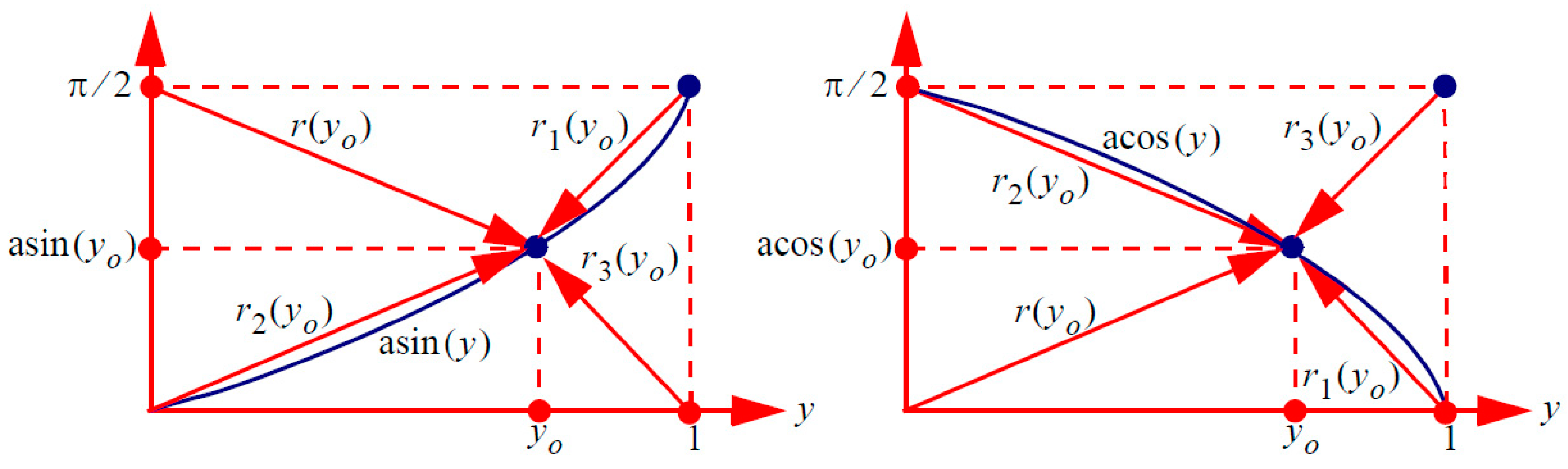
Consider the geometry, as illustrated in Figure 3, associated with arcsine and arccosine and which underpins the four radial functions defined according to
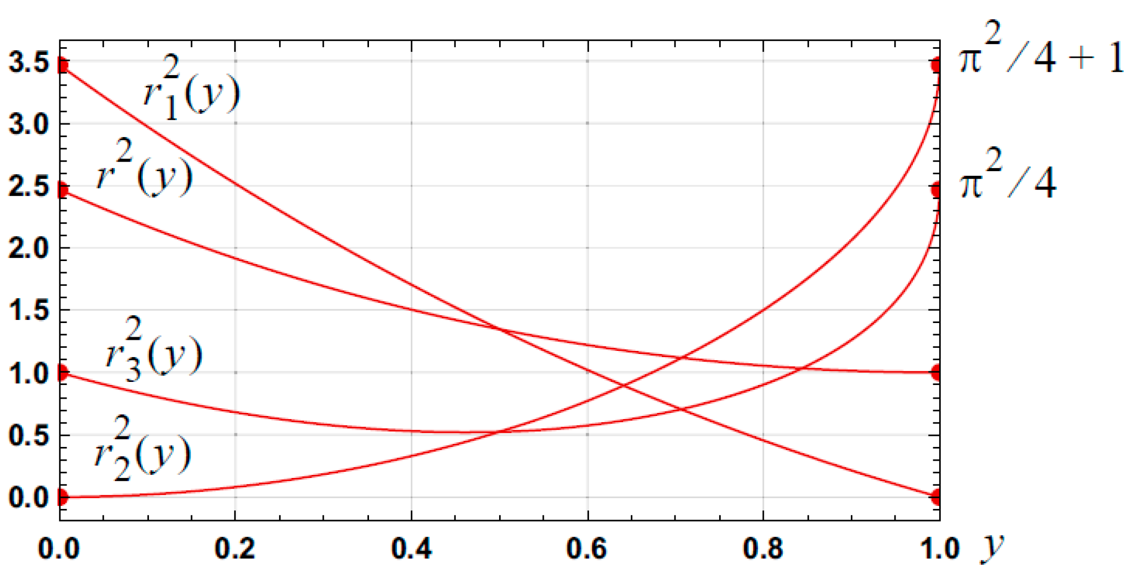
The graphs of these functions are shown in Figure 4. The functions and have undefined derivatives at the point , which does not facilitate function approximation. The function r2 is smoother than and can be utilized as a basis for approximation. If there exists an nth order approximation, , to , then the relationships , and can be utilized to establish approximations for arccosine, arcsine and arctangent.
3.1. Approximations for Radial Function
The two point spline approximation detailed in [15] (eqn. 40), and the alternative form given in [16] (eqn. 70) can be utilized to establish convergent approximations to the radial function defined by Equation (18).
Theorem 1.
Two Point Spline Approximations for Radial Function.
The nth order two point spline approximation to the radial function
, based on the points zero and one, is
where the coefficients are defined according to:
Here
and
. The derivative values of , at the points zero and one, are defined according to
Proof.
The proofs for these results are detailed in Appendix F. □
3.1.1. Notes on Coefficients
As , , and , , it follows that
As , , , , and , it is the case that for , . Hence, for fixed, , the magnitudes of both even and odd order coefficients monotonically decrease as increases and for .
3.1.2. Explicit Approximations
Explicit approximations for , of orders zero and one, are:
Higher order approximations, up to order six, are detailed in Appendix B along with the relevant coefficients , (see Table A1).
3.1.3. Approximations for Arccosine, Arcsine and Arctangent
With the definition of
the approximations, as stated in Corollary 1, follow.
Corollary 1.
Approximations for Arccosine, Arcsine and Arctangent.
The approximations for arccosine, arcsine and arctangent arising from the approximations specified in Theorem 1 are:
for . The superscript denotes alternative approximation forms. For the case of , the upper limit of the summations is rather than 1.
Proof.
These results follow directly from the definition (Equation (18)), and the approximations detailed in Theorem 1, leading to
The approximations for the other results arise from the fundamental relationships detailed in Equations (2)–(4), and according to
□
3.1.4. Explicit Approximations for Arccosine, Arcsine and Arctangent
Explicit approximations for arccosine, of orders zero, one and two, are:
Approximations, of orders three to six, are detailed in Appendix C. Explicit approximations for arcsine, of orders zero to six, can then be specified by utilizing the relationships and , . Explicit approximations for arctangent follow from the relationships and , . For example, the second order approximation for arctangent is
3.1.5. Relative Error Bounds for Arcsine, Arccosine and Arctangent
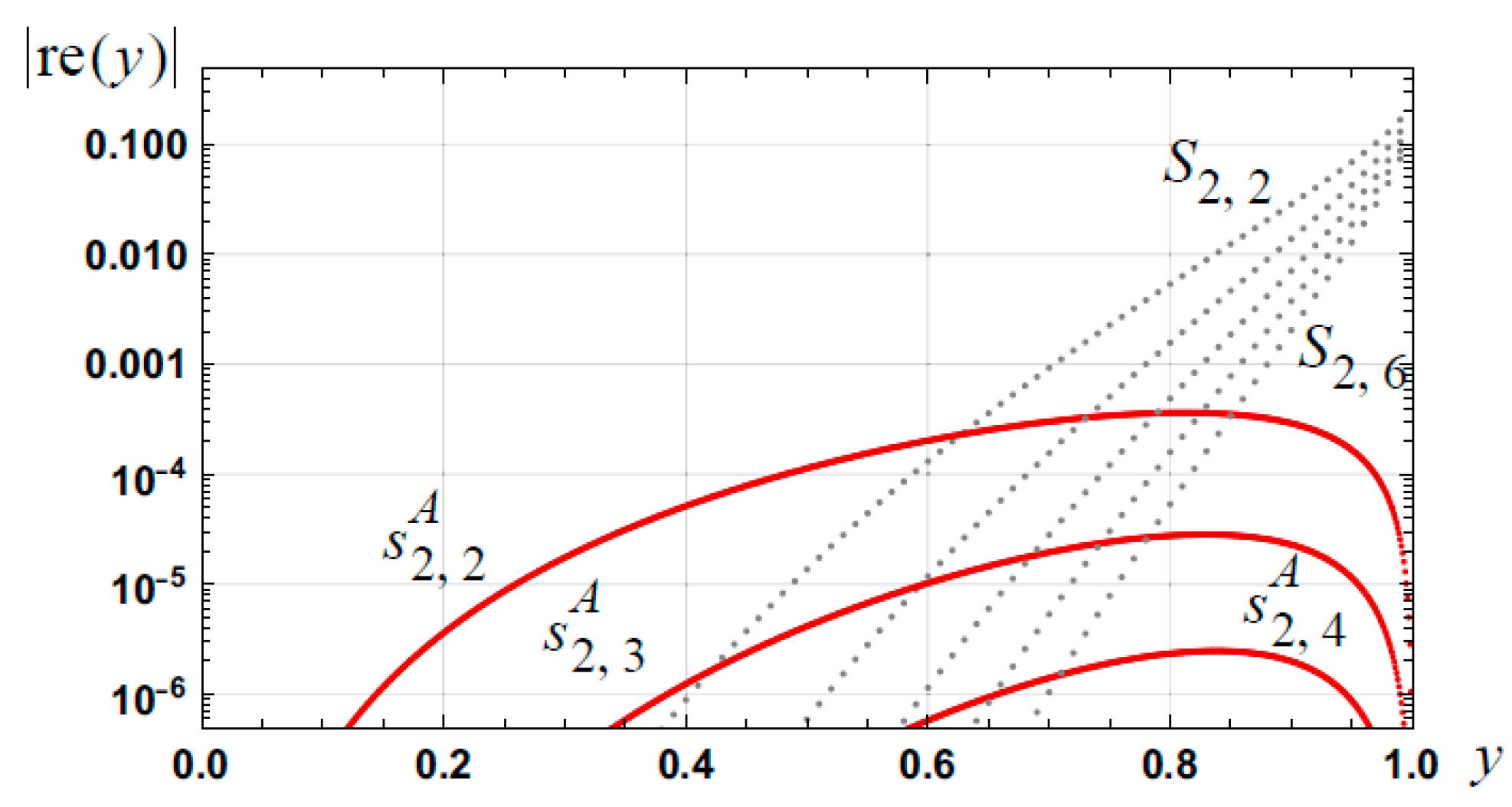
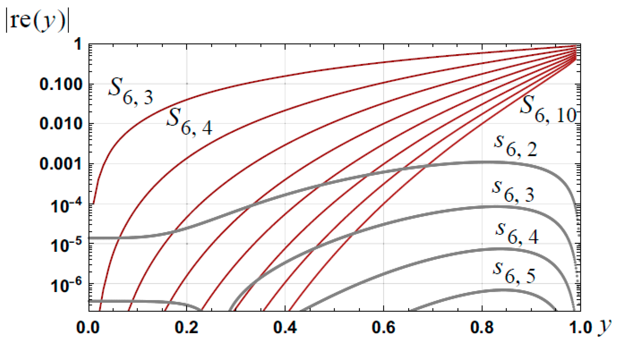
The relative error bounds for the approximations to , arcsine, arccosine and arctangent, arising from the approximations stated in Theorem 1 and Corollary 1 are detailed in Table 1. The relative errors in the approximations, of orders one to five, for arcsine, arccosine and arctangent are shown in Figure 5 and Figure 6. For example, the relative error bound associated with the fourth, , and sixth, , order approximations to arcsine, respectively, are and .
3.2. Alternative Approximations I: Differentiation of Arccosine Squared
Based on differentiation of the square of arccosine, alternative approximations for arccosine, arcsine and arctangent can be determined.
Theorem 2.
Alternative Approximations I: Differentiation of Arccosine Squared.
Alternative approximations, of order , for arcsine and arccosine, over the interval [0, 1], and arctangent, over the interval [0, ∞), are:
where , , with being defined by Equation (29).
Proof.
Consider the nth order approximation for arccosine, as defined in Corollary 1: , where , . Assuming convergence, it follows that . Differentiation yields
which implies
after the index change of and where . The approximation, defined by , for arcsine follows from the relationship ; the approximation for arctangent, defined by , follows according to
The alternative approximations follow according to
□
3.2.1. Note
The same approximations can be derived by considering the relationship which implies
Use of the arctangent approximation, , specified in Corollary 1 leads to the approximation
after the change of index . This result is consistent with stated in Theorem 2.
3.2.2. Explicit Approximations for Arcsine and Arctangent
Approximations for arcsine, of orders one and two, are
Approximations, of orders three and four, are detailed in Appendix D. As an example, the approximations for arctangent, of order two, are:
3.2.3. Results
3.2.4. Notes
The form of the approximation, as stated in Theorem 2, for arcsine:
is consistent with the optimum Padè approximant form specified by Abramowitz [14] and stated in Equation (15). The relative error bound for the Abramowitz approximation is . The relative error bound for the 4th order approximation, , as specified by Equation (A27), is whilst a fifth order approximation, , has a relative error bound of .
3.3. Alternative Approximations II: Integration of Arcsine
The integral of arcsine, e.g., [8] (4.26.14, p. 122), is:
which implies
There is potential with this relationship, and based on approximations to arcsine that are integrable, to define new approximations to arcsine, with a lower relative error bound, than the approximations detailed in Corollary 1 and Theorem 2. The approximations to arcsine, as defined by , in Theorem 2, are integrable and lead to the following approximations.
Theorem 3.
Alternative Approximations II—Integration of Arcsine.
Alternative approximations, of order , , for arcsine, arccosine and arctangent, are:
where with being defined by Equation (29).
Proof.
Consider the approximation for arcsine defined by and stated in Theorem 2. Use of this approximation in Equation (53) leads to
The result
leads to the approximation defined in Equation (54). The alternative approximations follow according to . □
3.3.1. Explicit Approximations for Arcsine
A second order approximations for arcsine is:
and has a relative error bound of . A fourth order approximation has a relative error bound of .
3.3.2. Results
The relative error bounds associated with the approximations , and to arcsine, arccosine and arctangent, as specified by Theorem 3, are detailed in Table 3. The relative errors associated with , and become unbounded, respectively, at the points zero, one and zero. The graphs of the relative errors for and are shown in Figure 10.
3.4. Alternative Approximations
Alternative approximations can be determined. For example, the relationship:
leads to a quadratic equation for arcsine when an integrable approximation for is utilized. As a second example, the relationship
implies
and, thus, an approximation for arcsine can be determined when a suitable approximation for , which is integrable, is available.
4. Error and Convergence
Consider the definition of the square of the radial function as defined by Equation (18) and the error in the order approximation, , to , as defined in Theorem 1, i.e.,
Consistent with the nature of a order two point spline approximation based on the points zero and one, it is the case that .
From Equation (63) it follows that
where is the order approximation to arccosine defined in Corollary 1 and the error in this approximation is . For fixed, and for the convergent case where , it is the case that . Hence, for fixed, convergence of to as increases, is sufficient to guarantee the convergence of to .
Consider the order approximation to arcsine, , as given in Corollary 1. It then follows that
Again, for fixed, a sufficient condition for convergence of to is for .
As , it follows that the error in the approximation, , to arctangent, as given by Corollary 1, yields the relationship
and, thus, . Again, for y fixed, convergence of to atan(y) is guaranteed if .
The goal, thus, is to establish convergence of the approximations specified by Theorem 1, i.e., to show that . To achieve this goal, the approach is to determine a series for the error function and this can be achieved by first establishing a differential equation for .
4.1. Differential Equation for Error
Consider Equation (64): . Differentiation yields
and after squaring and simplification the equation becomes
Rearrangement leads to the differential equation for the error function:
A polynomial expansion can be used to solve for .
Theorem 4.
Polynomial Form for Error Function.
A polynomial form for the error function, , as defined by the differential equation specified in Equation (69), is
where is the coefficient defined in Theorem 1 and.
Proof.
The proof is detailed in Appendix E. □
Explicit Approximations
Polynomial expansions for , of orders three and four, are:
4.2. Convergence
First, consistent with Equation (22), . Second, consistent with Equation (26), it is the case that
As discussed in Section 3.1.1, it is the case that and with for . It then follows that and the decrease in magnitude is monotonic as increases for even and odd values. Third, from Equation (70) and the result , it follows, for the case of , fixed, that
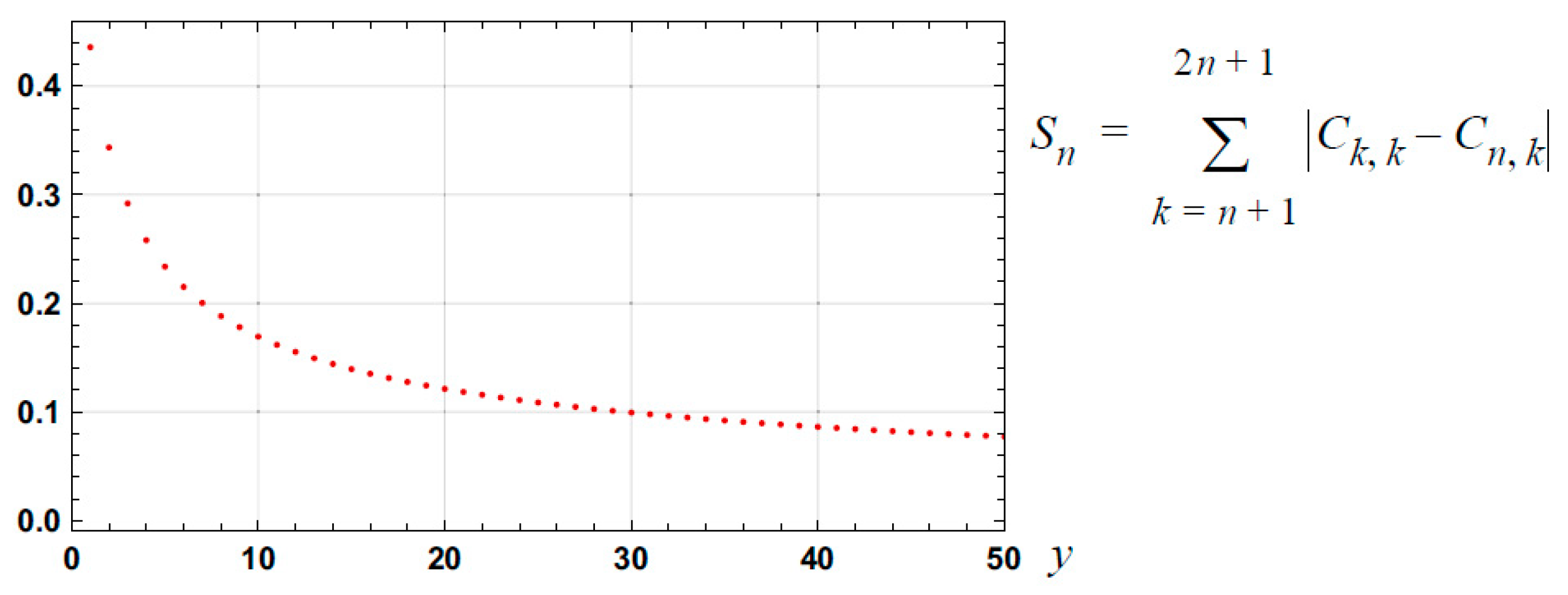
The graph of is shown in Figure 11. As this is bounded, and as , it follows that for .
5. Direct Approximation for Arctangent
The approximations for arctangent detailed in Corollary 1, Theorem 2 and Theorem 3 are indirectly established. Direct approximations for arctangent can be established by utilizing the fundamental relationships , which implies
5.1. Approximations for Arctangent
The following theorem details a spline based approximation for arctangent.
Theorem 5.
Approximations for Arctangent.
Given a
order spline based approximation, , for ,
, based on the points zero and one, it is the case that
The resulting order approximation, , , for arctangent is
where the coefficients , , are defined according to:
Here:
where and
Proof.
Consider the approximation for , . The relationship implies
The formulas for , and can be established in a manner consistent with the nature of the proof detailed in Appendix F. □
5.1.1. Analytical Approximations
Approximations for arctangent, of orders zero to two, are:
Approximations, of orders three and four, are detailed in Appendix G.
5.1.2. Approximations for Arccosine and Arcsine
The relationships and , , imply the following approximations for arcsine and arccosine:
Alternative approximations for arcsine and arccosine specified according to and lead to identical expressions, i.e., and .
As an example, the third order approximation for arcsine is
5.1.3. Results
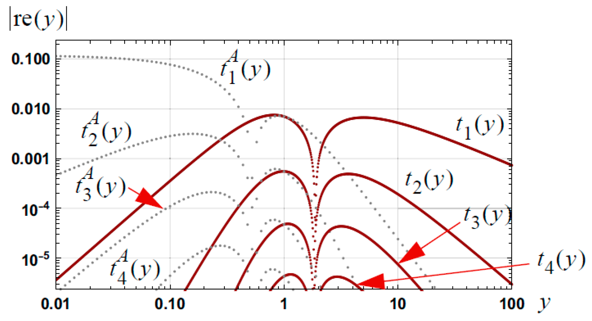
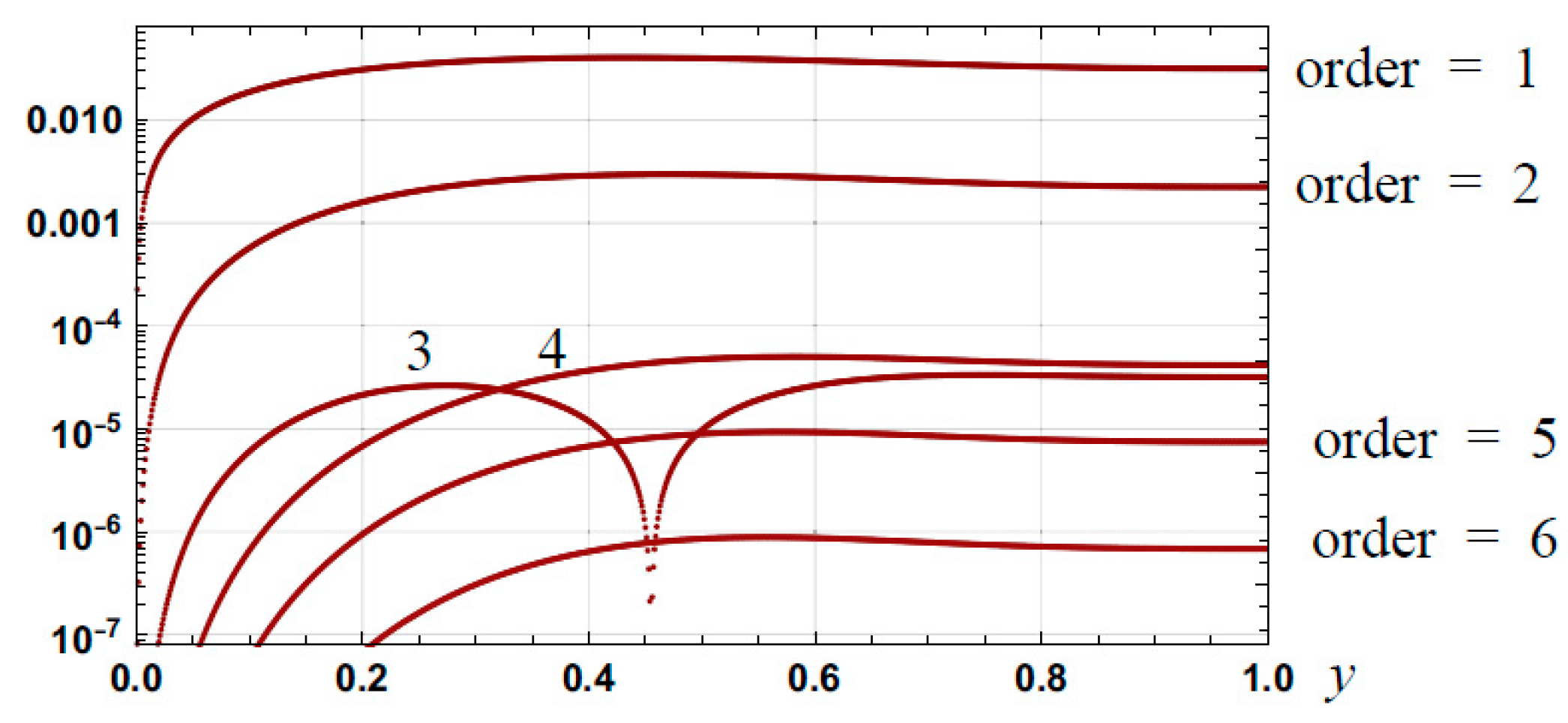
The relative errors associated with the approximations for arctangent, of orders one to six, are shown in Figure 12. The relative error bounds associated with the approximations to arctangent, arcsine and arccosine are detailed in Table 4. The relative error bound associate with the third order approximation for arcsine, as specified by Equation (88), is 3.73 × 10⁻⁵ which is comparable with the third order approximation specified in Corollary 1 whose relative error is 2.84 × 10⁻⁵.
5.2. Improved Approximation: Use of Integral for Arctangent
Consider the known integral
which implies
An integrable approximation for , for , leads to an approximation for arctangent.
Theorem 6.
Improved Approximations for Arctangent.
The nth order approximation for arctangent, based on Equation (90), is defined according to
where the coefficients
are defined in Equation (78) and
Here is associated with and with the first value being exact. The second value yields a lower relative error bound for the interval .
Proof.
The approximations for arctangent, as defined in Theorem 5, when used in the integral in Equation (90), lead to the approximations specified by Equation (91). □
5.2.1. Explicit Expressions
Explicit approximations for arctangent, of orders one and two, are:
Third and fourth order approximations are detailed in Appendix H.
Explicit approximations for arcsine and arccosine can be defined by utilizing the relationships and .
5.2.2. Results
The relative error bounds associated with the approximations to arctangent are detailed in Table 4 and the improvement over the original approximations is evident.
6. Improved Approximations via Iteration
Given an initial approximating function for the inverse,, of a function , the iteration of the classical Newton-Raphson method of approximation leads to the order approximation
6.1. Newton-Raphson Iteration: Approximations and Results for Arcsine
The arcsine case is considered: An initial approximation to arcsine of , as specified by Corollary 1, Theorem 2, Theorem 3 or Section 5.1.2, leads to the order iterative Newton-Raphson approximation:
Iteration of orders one and two lead to the approximations:
The approximation arising from a third order iteration is detailed in Appendix I.
Example and Results
As an example, consider the second order approximation for arcsine arising from Theorem 2 and defined by Equation (49):
The relative error bound associated with this approximation is . The first order iteration of the Newton-Raphson method yields the approximation
The relative error bound for this approximation, and associated with the interval [0, 1], is . Second order iteration yields the approximation detailed in Equation (A62). The relative error bound associated with this approximation, for the interval [0, 1], is The use of , as specified by Equation (A27), rather than leads to a relative error bound of .
Consider the fourth order approximation, , defined by Equation (A27). A first order iteration of the Newton-Raphson method yields the approximation
The relative error bound associated with this approximation is .
The improvement that is possible with Newton-Raphson iteration is illustrated in Table 5 where the original approximations to arcsine and arctangent, based on , , and as defined in Theorem 2 and specified by Equations (49) and (50), are used. The quadratic convergence, with iteration, is evident. It is usual for the relative error improvement, with iteration, to be dependent on the relative error in the initial approximation. However, as the results in Table 5 indicate, the approximations of and , with higher relative error bounds, lead to lower relative bounds with iteration than and . This is due to the nature of the approximations.
7. Applications
7.1. Approximations for a Set Relative Error Bounds: Arcsine
With the requirement of a set relative error bound in an approximation for arsine, arccosine or arctangent, an approximation form and a set order of approximation can be specified. The following details examples of approximations for arcsine and the interval [0, 1] is assumed.
For a relative error bound close to 10−4, the approximation
as given by Corollary 1, yields a relative error bound of 1.81 × 10⁻⁴. The approximation, , defined by Equation (59) yields a relative error bound of 1.56 × 10⁻⁴.
For a relative bound close to 10−6, the approximation , where is defined by Equation (A22), is
and has a relative error bound of 2.49 × 10⁻⁶. The approximation defined by (see Equation (A14)) is
and has a relative error bound of 1.19 × 10⁻⁶. The approximation given by Abramowitz, as stated in Equation (15), has a relative error bound of 3.04 × 10⁻⁶.
If a high accuracy approximation is required then two approaches can be used. First, higher order approximations as specified in Corollary 1, Theorem 2, Theorem 3 and Theorem 5 can be used. For example, the fifteenth order approximation, , for arcsine detailed in Corollary 1 yields a relative error bound of 4.74 × 10⁻¹⁷. Second, iterative approaches can be used. For example, the second order approximation, , for arcsine arising from Theorem 2 and defined by Equation (49) and a second order iteration leading to Equation (A62) has a relative error bound of 5.68 × 10⁻¹⁵. An alternative approximation can be defined by utilizing the zero order spline approximation, as specified by Equation (117), and the sixth and seventh order approximations (the function ) which yields a relative error bound of 7.65 × 10⁻¹⁸ (see Table 6).
7.2. Upper and Lower Bounds for Arcsine, Arccosine and Arctangent
Lower, , and upper, , bounds for arcsine, i.e.,
lead to the following lower and upper bounds for arccosine and arctangent:
7.2.1. Published Bounds for Arcsine
There is interest in upper and lower bounds for arcsine, e.g., [17,18,19,20,21]. The classic upper and lower bounded functions for arcsine are defined by the Shafer-Fink inequality [13]:
The relative error bound associated with the lower bounded function is ; the relative error bound associated with the upper bounded function is .
Zhu [20] (eqn. 1.8), proposed the bounds:
where the lower relative error bound is and the upper relative error bound is .
Zhu [21] (Theorem 1), proposed the bounds
The lower bound is equivalent to the bound proposed by Maleševí et al. [19] (eqn. 21). The relative errors in the bounds are low for but increase as increases. For the case of the relative error bound for the lower bounded function is 0.0324; for the upper bounded function the relative error bound is 0.0159.
7.2.2. Proposed Bounds for Arcsine and Arccosine
Consider the approximations defined in Corollary 1 and whose relative errors are shown in Figure 5. As the graphs in this figure indicate, the approximations are either upper or lower bounds for arcsine and arccosine and this is confirmed by numerical analysis (for the orders considered) which shows that there are no roots, in the interval (0,1), for the error function associated with the approximations. The evidence is that the approximations, , of orders 0, 2, 4, …, are lower bounds for arcsine whilst the approximations of orders 1, 3, 5, … are upper bounds. Thus, for example, second, , and third, , order approximations, as defined in Corollary 1, yield the inequalities
for , where, as detailed in Table 1, the lower relative error bound is 3.64 × 10⁻⁴ and the upper relative error bound is 2.84 × 10⁻⁵.
It then follows, from Equation (106), that
for . An analytical proof that the approximations for arcsine and arccosine, as detailed in Corollary 1, are upper/lower bounds is an unsolved problem.
7.2.3. Upper/Lower Bounds for Arctangent
As an example of upper and lower bounds that have been proposed for arctangent, consider the bounds proposed by Qiao and Chen [22] (Theorem 3.1 and Theorem 4.2) for y > 0:
The lower bounded function in Equation (114) has a relative error bound of 0.0520; the upper bounded function has a relative error bound of 0.0274. The error in the upper and lower bounded functions specified in Equation (115) diverges as y → 0 but converges rapidly to zero for .
7.2.4. Proposed Bounds for Arctangent
As it follows, from Equation (113), that the functions and defined in Corollary 1 are, respectively, upper and lower bounds for arctangent, i.e.,
for As detailed in Table 1, the relative error bound for the lower bounded function is 1.42 × 10⁻⁵ and 1.81 × 10⁻⁴ for the upper bounded function.
7.3. Spline Approximations Based on Upper/Lower Bounds
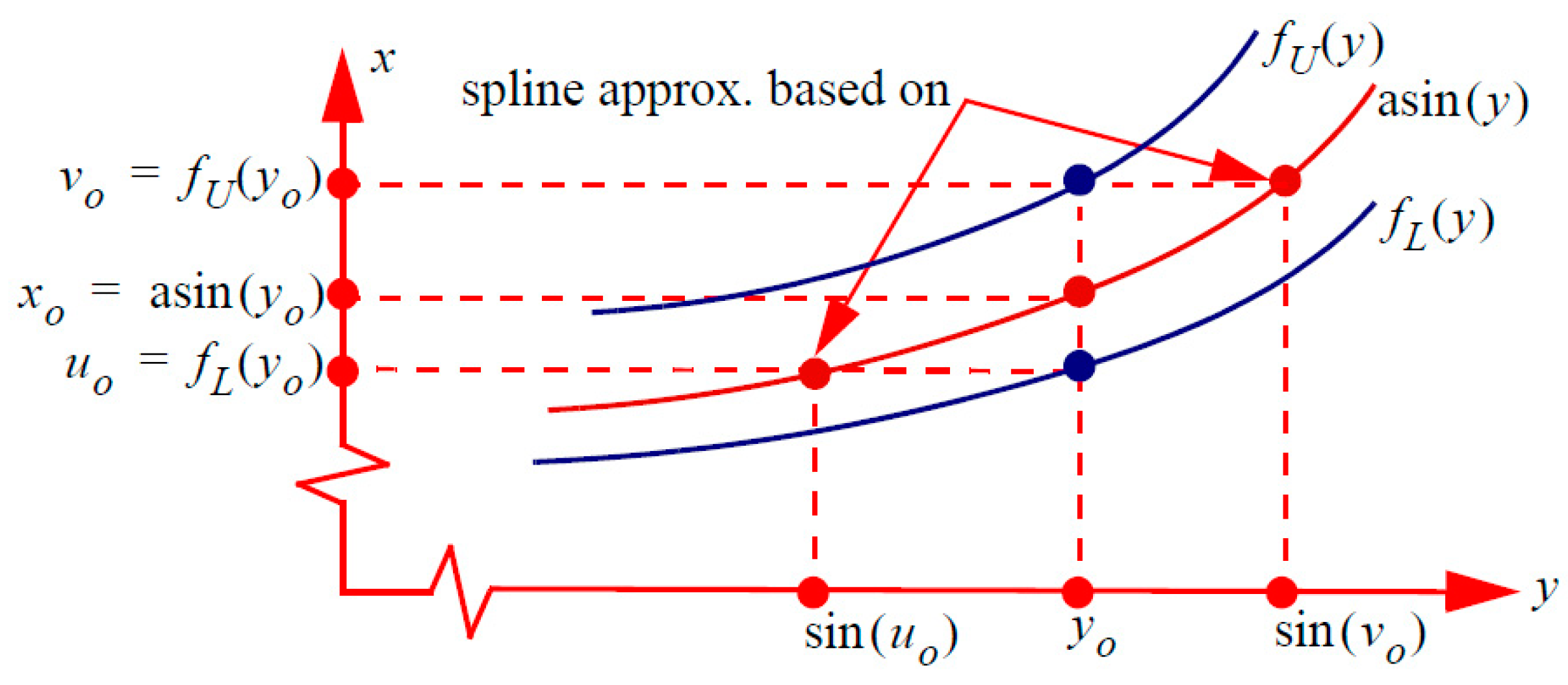
Consider upper, , and lower, , bounded functions for arcsine as illustrated in Figure 13. For fixed at a spline approximation, based on the points , and ,, can readily be determined. From such an approximation, an approximation to can then be determined.
Theorem 7.
Spline Approximations Based on Upper/Lower Bounds.
Consider lower,, and upper,, bounded approximations for arcsine. The zero order spline approximation for arcsine, based on the approximationsand, is
The
order spline approximation for arcsine, based on the approximationsand,
is
for , , , and
where
and for :
Proof.
The proof is detailed in Appendix J. □
Results
Consider the approximations the approximation , , for arcsine as detailed in Corollary 1 where approximations, of order 0, 2, 4, …, are lower bounds and the approximations, of orders 1, 3, 5, …, are upper bounds. For example, with and , with and defined by Equation (A22) and Equation (A23), the zero order spline approximation, as specified by Equation (117), is
The relative error bound for this approximation, over the interval , is . Other results are detailed in Table 6 and clearly show the high accuracy of the approximations.

Table 6.
Relative error bounds, over the interval , for spline approximations based on upper and lower bounded approximations to arcsine and as specified in Theorem 7.
Table 6.
Relative error bounds, over the interval , for spline approximations based on upper and lower bounded approximations to arcsine and as specified in Theorem 7.
| Upper/Lower Bounded Functions: | Spline Order | Notation for Approx. | Relative Error Bound |
|---|---|---|---|
| 0 | |||
| 1 | |||
| 2 | |||
| 3 | |||
| 4 | |||
| 0 | |||
| 1 | |||
| 2 | |||
| 3 | |||
| 4 | |||
| 0 | |||
| 1 | |||
| 2 | |||
| 3 | |||
| 4 | |||
| 0 | |||
| 1 | |||
| 2 | |||
| 3 | |||
| 4 |
7.4. Approximations for Arcsine Squared and Higher Powers
There is interest in approximations for , , , , e.g., [23,24,25,26]. The standard series for , e.g., [7] , is
The nth order approximation,, specified in Corollary 1, leads to the approximations for defined according to
for . The relative errors in and are shown in Figure 14. The approximations defined by have better overall relative error performance; in particular, they are sharp at the point one.
7.4.1. Approximations for Even Powers of Arcsine
Based on the approximation for the square of arcsine, as specified by Equation (124), the following result can be stated:
Theorem 8.
Approximation for Even Powers of Arcsine.
Based on the nth order approximation, , specified in Corollary 1, the even powers of arcsine can be approximated according to
where
Here, are defined by Equation (29).
Proof.
This result follows from expansion of to the 2mth power, i.e.,
and collecting terms associated with .□
7.4.2. Example
For example, the nth order approximation for is
7.4.3. Roots of Arccosine: Approximations for Even Powers of Arccosine and Arcsine
The following theorem details a better approach for evaluating approximations for and , .
Theorem 9.
Root Based Approximation for Even Powers of Arccosine and Arcsine.
Approximations of order , for and , , respectively, are
where
is the conjugate of
and
are the roots of the
th order approximation
to defined in Corollary 1.
Proof.
Consider the nth order approximation to defined in Corollary 1. This approximation is denoted and is of the form
This approximation can be written in the form
It then follows that
The approximation, , for arises from the relationship . □
7.4.4. Approximations for Arccosine Squared
The second order approximation for is
where . The relative error bound for this approximation, over the interval [0, 1], is 3.66 × 10⁻⁴. The fourth and sixth order approximations are detailed in Appendix K and have the respective relative error bounds of 2.48 × 10⁻⁶ and 2.25 × 10⁻⁸. By using higher resolution in the approximations to the roots, slightly lower relative error bounds can be achieved. The stated root approximations represent a good compromise between accuracy and complexity.
7.4.5. Results
The relative error bounds associated with the order approximations for and are detailed in Table 7.
7.4.6. Comparison with Published Results
Borwein [23] details approximations for even powers of arcsine and approximations for powers of two, four, six, eight and ten are detailed in Appendix L. The approximation for arcsine to the sixth power is
As an example, the relative error in approximations for , as defined by (Equation (130)) and the Borwein approximation , are shown in Figure 15. The clear advantage of the root based approach over the series defined by is evident. In particular, the root based approximations are sharp at the point one.
7.5. Approximations for the Inverse Tangent Integral Function
The inverse tangent integral function is defined according to
and an explicit series form (e.g., Mathematica) is
The Taylor series for arctangent, as given by Equation (7), leads to the order approximation, , for :
where is the unit step function. The relative error in approximations, of orders one to ten, are shown in Figure 16.
7.5.1. Inverse Tangent Integral Approximation
Based on the nth order approximation for arctangent, , stated in Theorem 2, a nth order approximation to the inverse tangent integral is
where is defined in Theorem 2 and the integrals, are defined according to
The first order approximation, for the inverse arctangent integral, is
Second and third order approximations are detailed in Appendix M.
7.5.2. Notes and Relative Error
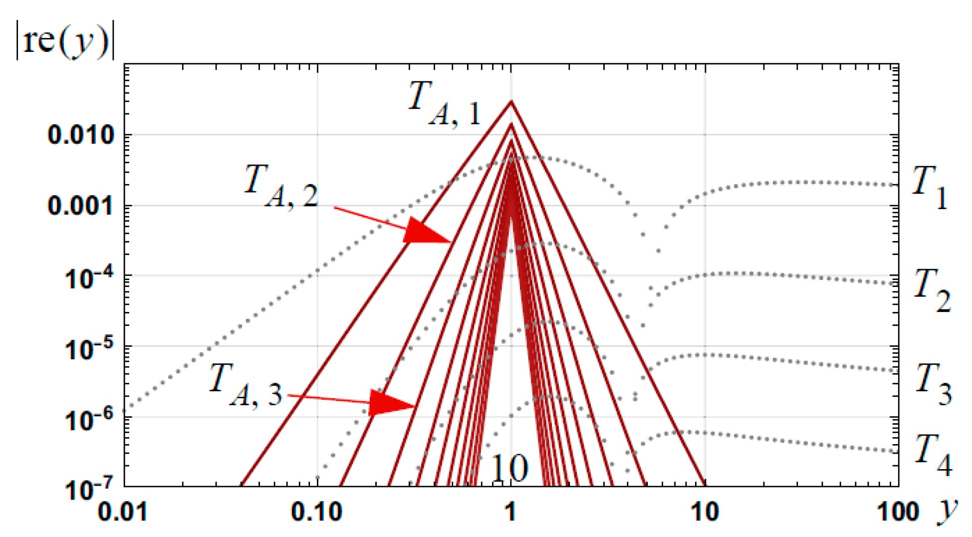
The approximations, , , are valid over the positive real line and the relative error in the approximations, of orders one to four, are shown in Figure 16. As is evident in this Figure, the approximations have a lower relative error bound than the disjointly defined Taylor series approximations defined by Equation (138). The relative error bounds associated with the approximations are detailed in Table 8.
7.5.3. Approximation of Catalan’s Constant
As Catalan’s constant can be defined according to
it follows that approximations for this constant, of orders two and four, can be defined according to
The respective relative errors in these approximation are and .
7.6. Approximations for Unknown Integrals
The different forms for the approximations for arcsine, arccosine and arctangent, potentially, can lead to approximations for unknown integrals involving these functions. Four examples are detailed below.
7.6.1. Example 1
The function is an approximation to the unit step function for after a transient rise time. Using the approximation form, , detailed in Corollary 1 for arccosine, the approximation to the integral of this function (scaled by ) can be defined:
.
The third order approximation is
and the relative error bound associated with this approximation, over the interval , is .
7.6.2. Example 2
Using the approximation form, , detailed in Corollary 1 for arctangent, the following approximation can be defined
Mathematica, for example, specifies this integral in terms of the poly-logarithmic function. The third order approximation is
and the relative error bound associated with this approximation, over the interval , is .
7.6.3. Example 3
The following integral does not have an explicit analytical form but the approximations, , detailed in Corollary 1, leads to
, where the polynomials can readily be established. For the case of , the relative error bound, associated the interval , is .
7.6.4. Example 4
Consider the definite integral defined by Sofo and Nimbran [27] (example 2.8, factor of 1/4 missing):
The polynomial approximation, , for arctangent detailed in Theorem 5 and for the interval , yields
for . For the case of the approximation is
The relative errors in the approximations and are detailed in Table 9. The relative errors in the approximations
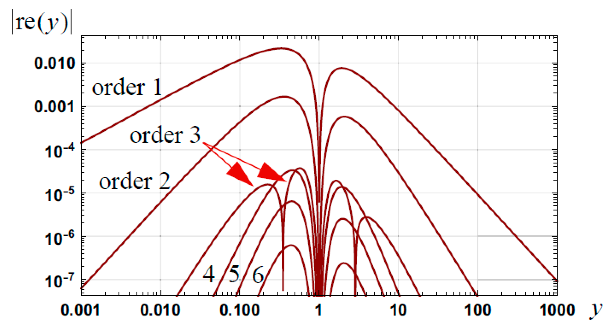
, ,6} are shown in Figure 17. From the results shown in Table 9, it is clear that the approximations specified by Equation (154) converge significantly faster than the approximations detailed by Sofo and Nimbran [27] (Equation (152)). In addition, the approximation, , for arctangent, underpins the more general approximation, as specified by Equation (153), for the integral I, .
8. Summary and Conclusions
8.1. Summary of Results
The approximations detailed in the paper for arcsine and arctangent are tabulated, respectively, in Table 10 and Table 11.
For arcsine, the approximation form, detailed in Theorem 2, can be written in the simple form
where and are polynomial functions. The approximation , detailed in Theorem 3, has the lowest relative error bound for a set order (e.g., order four).
8.2. Conclusions
Based on the geometry of a radial function, and the use of a two point spline approximation, approximations of arbitrary accuracy, for arcsine, arccosine and arctangent, can be specified. Explicit expressions for the coefficients used in the approximations were detailed and convergence was proved. The approximations for arcsine and arccosine are sharp at the point zero and one and have a defined relative error bound for the interval . Alternative approximations were established based on a known integration result and a known differentiation result. The approximations have the forms detailed in Table 10 and Table 11.
By utilizing the anti-symmetric relationship for arctangent around the point one, a two point spline approximation was used to establish approximations for this function as well as for arcsine and arccosine. Alternative approximations were established by using a known integral result.
Iteration utilizing the Newton-Raphson method, and based on any of the proposed approximations, yields results with significantly higher accuracy. The approximations exhibit quadratic convergence with iteration.
Applications of the approximations include: first, upper and lower bounded functions, of arbitrary accuracy, for arcsine, arccosine and arctangent. Second, it was shown how to use upper and lower bounded approximations to define approximations with significantly higher accuracy. Third, it was shown that the approximation , detailed in Corollary 1, leads to a simple approximation form for the square of arcsine which has better convergence than established series for this function. By utilizing the roots of the square of the approximations to arccosine detailed in Corollary 1, it was shown how approximations to arccosine and arcsine, to even power orders, can be established. It was shown that the relative error bounds associated with such approximations are significantly lower that published approximations. Fourth, approximations for the inverse tangent integral function were proposed which have significantly lower relative error bounds over the interval , than established Taylor series based approximations. Fifth, the approximation forms for arccosine and arctangent were utilized to establish approximations to several unknown integrals.
Funding
This research received no external funding.
Institutional Review Board Statement
Not relevant.
Informed Consent Statement
Not applicable.
Conflicts of Interest
The author declares no conflict of interest.
Appendix A. Approximations Based on Angle Subdivision
Given the coordinate of a point on the first quadrant of the unit circle, and the corresponding angle , as defined by and , the following definitions can be made:
Algorithms for determining and arise from half-angle formulas and are:
The following result can be proved, following the approach detailed in [15] (Section 6.4 and Appendix I).
Theorem A1.
Approximation for Arcsine and Arccosine.
Approximations for
and
, of order
, are:
where
Proof.
The angle
can be defined according to the standard path length formula along the unit circle from the point to the point (the point consistent with the angle ):
The integral can be approximated by using the general integral approximation [15] (eqn. 14):
where for the case being considered
Here,
is specified by Equation (A5). For the case of
and
or , Equation (A8), respectively, leads to the required results:
□
Explicit Approximations for Arccosine
Some examples of the approximations for arccosine, as specified by Equation (A4), are detailed below: First, based on , the second order spline approximation yields
which has a relative error bound, for the interval of . Second, based on , the second order spline approximation yields
which has a relative error bound, for the interval , of . Third, based on , the first order spline approximation yields
which has a relative error bound, for the interval , of .
Appendix B. Explicit Approximations for Radial Function
Approximations for , as specified by Theorem 1 and of orders one to six, are detailed below with the coefficients , , being specified in Table A1:
Table A1.
Table of coefficients. The lower order coefficients that are not listed are defined according to .
Table A1.
Table of coefficients. The lower order coefficients that are not listed are defined according to .
| Order of Approx. | Coefficients |
|---|---|
| 0 | |
| 1 | |
| 2 | |
| 3 | |
| 4 | |
| 5 | |
| 6 |
Appendix C. Explicit Approximations for Arccosine
Explicit approximations for arccosine, of orders three to six and arising from Corollary 1, are:
Appendix D. Approximations for Arcsine of Orders Three to Four
Approximations for arcsine, of orders three and four and arising from Theorem 2, are:
Appendix E. Proof of Theorem 4
Consider the differential equation stated in Equation (68):
and the nth order approximation, , detailed in Theorem 1: . As , the following form for the error function is assumed:
with unknown coefficients .
Use of this form in Equation (A29) leads to
i.e.,
As , , it follows that the coefficients , , are independent of , leading to
By sequentially considering the coefficients of
the constants , , can be determined. First, the coefficient of yields , leading to . The negative solution is required as
and
. Second, the coefficient of
yields
, leading to . Third, the coefficient of yields , leading to . For the general case, the coefficient of , , yields
Thus:
i.e.,
leading to
for .
Coefficient Values
Use of Equation (A37), for , leads to the following list of coefficient values:
and the values are consistent with the result , for (see Table A1 for , , …, ). It is the case that . These results are consistent, see Equation (A30), with the requirement that , which implies , .
From Equation (A30), the result , then follows and, for , it is the case that
which is the required result.
Appendix F. Proof of Theorem 1
Consider the form for the order two point spline approximation, denoted , to a function
as detailed in [15] (eqn. 40), and the alternative form given in [16] (eqn. 70). Based on the points zero and one, the order approximation is
, where , .
The sequence of numbers defined by and , for , respectively, are:
For the first sequence, the ratios of the fifth to the third term, the seventh to the fifth term, ... are:
The ratios of the sixth to the fourth term, eight to the sixth term, are:
It then follows that the general iteration formula for is:
The general iteration form for
arises by considering the ratios , for , leading to:
Appendix F.1. Formula for Coefficients in Standard Polynomial Form
The goal is to write the approximation , as defined by Equation (A40), in the form
To this end, the binomial formula
implies
Thus:
For , is associated with the value of k in the summation
which is such that , k ≥ 0, i.e., and . Thus:
For , the lowest value of , such that there is a term associated with in , satisfies the constraint , i.e., . The term is also associated with the index , , in bn,r, i.e., , and with the lowest value of being consistent with . Thus:
Appendix F.2. Nature of Coefficients
Consider and as defined by Equations (A41) and (A52), whereupon it follows that
It can readily be shown that
This result is consistent with the requirement,
for , associated with a two point spline approximation of order .
Appendix G. Third and Fourth Order Approximations for Arctangent
Approximations for arctangent, of orders three and four and arising from Theorem 5, are:
Appendix H. Alternative Third and Fourth Order Approximations for Arctangent
Third and fourth order approximations for arctangent, and arising from Theorem 6, are:
Appendix I. Additional Approximations for Arcsine via Iteration
The third order iteration, arising from Equation (96), leads to the following approximation for arcsine:
The second order iteration, based on Equation (99), leads to the following approximation for arcsine:
Appendix J. Proof of Theorem 7
A zero order spline approximation is simply an affine approximation between the two specified points. Consistent with the illustration of Figure 13, the zero order spline approximation, denoted , to , is an affine approximation between the points and leading to
With the approximation it follows, after simplification, that
Substitution of and yields the required result after the change in variable from
to y.
General Result
Consider the general order spline approximation to a function over the interval , as given by [16] (eqn. 70):
where
The general result stated in Theorem 7 arises with the definitions , and the interval
where , and , . The approximation is
for and where is the derivative of arcsine. An analytical expression for arises from noting that and that has the form
where the coefficients are to be determined. By considering the forms for and , the algorithm for the coefficients, as specified in Theorem 7, can be determined. Qi and Zheng [28] detail an alternative form for . As and , it then follows that
for . The required result follows: the approximation for arises for the case of .
Appendix K. Fourth and Sixth Order Approximations for Arccosine Squared
The fourth and sixth order approximations for arccosine squared, consistent with Theorem 9, are:
Appendix L. Approximations for Even Powers of Arcsine
Borwein [23] (eqn. 2.2 to 2.4) details approximations for even powers of arcsine and the approximations for powers of two, four, six, eight and ten are:
Appendix M. Second and Third Order Approximations for Inverse Tangent Integral
Second and third order approximations for the inverse tangent integral are:
References
- Boyer, C.B. A History of Mathematics; John Wiley: New York, NY, USA, 1991. [Google Scholar]
- Bercu, G. The natural approach of trigonometric inequalities—Padé approximant. J. Math. Inequalities 2017, 11, 181–191. [Google Scholar] [CrossRef]
- Howard, R.M. Spline based series for sine and arbitrarily accurate bounds for sine, cosine and sine integral. arXiv 2020. [Google Scholar] [CrossRef]
- Stroethoff, K. Bhaskara’s approximation for the sine. Math. Enthus. 2014, 11, 485–492. [Google Scholar] [CrossRef]
- Ablowitz, M.J.; Kaup, D.J.; Newell, A.C.; Segur, H. Method for solving the Sine-Gordon equation. Phys. Rev. Lett. 1973, 30, 1262–1264. [Google Scholar] [CrossRef]
- Alkhairy, I.; Nagy, M.; Muse, A.H.; Hussam, E. The arctan-X family of distributions: Properties, simulation, and applications to actuarial sciences. Complexity 2021, 2021, 4689010. [Google Scholar] [CrossRef]
- Gradshteyn, I.S.; Ryzhik, I.M. Tables of Integrals, Series and Products, 7th ed.; Jeffery, A., Zwillinger, D., Eds.; Academic Press: Washington, DC, USA, 2007. [Google Scholar]
- Roy, R.; Olver, F.W.J. Elementary functions. In NIST Handbook of Mathematical Functions; Olver, F.W., Lozier, D.W., Boisvert, R.F., Clark, C.W., Eds.; National Institute of Standards and Technology: Gaithersburg, MD, USA; Cambridge University Press: Cambridge, UK, 2010; Chapter 4. [Google Scholar]
- Gómez-Déniz, E.; Sarabia, J.M.; Calderín-Ojeda, E. The geometric arcTan distribution with applications to model demand for health services. Commun. Stat. - Simul. Comput. 2019, 48, 1101–1120. [Google Scholar] [CrossRef]
- Scott, J.A. Another series for the inverse tangent. Math. Gaz. 2011, 95, 518–520. [Google Scholar] [CrossRef]
- Bradley, D.M. A class of series acceleration formulae for Catalan’s constant. Ramanujan J. 1999, 3, 159–173. [Google Scholar] [CrossRef]
- Wu, S.; Bercu, G. Padé approximants for inverse trigonometric functions and their applications. J. Inequalities Appl. 2017, 2017, 31. [Google Scholar] [CrossRef]
- Fink, A.M. Two inequalities. Univ. Beograd. Publ. Elektrotehn. Fak. Ser. Mat 1995, 6, 49–50. [Google Scholar]
- Abramowitz, M.; Stegun, I.A. (Eds.) Handbook of Mathematical Functions with Formulas, Graphs and Mathematical Tables; Dover: Garden City, NY, USA, 1964. [Google Scholar]
- Howard, R.M. Dual Taylor series, spline based function and integral approximation and applications. Math. Comput. Appl. 2019, 24, 35. [Google Scholar] [CrossRef]
- Howard, R.M. Analytical approximations for the principal branch of the Lambert W function. Eur. J. Math. Anal. 2022, 2, 14. [Google Scholar] [CrossRef]
- Bercu, G. Sharp refinements for the inverse sine function related to Shafer-Fink’s inequality. Math. Probl. Eng. 2017, 2017, 9237932. [Google Scholar] [CrossRef]
- Guo, B.N.; Luo, Q.M.; Qi, F. Sharpening and generalizations of Shafer-Fink’s double inequality for the arc sine function. Filomat 2013, 27, 261–265. [Google Scholar] [CrossRef]
- Maleševí, B.; Rašajski, M.; Lutovac, T. Refinements and generalizations of some inequalities of Shafer-Fink’s type for the inverse sine function. J. Inequalities Appl. 2017, 2017, 275. [Google Scholar] [CrossRef]
- Zhu, L. New inequalities of Shafer-Fink type for arc hyperbolic sine. J. Inequalities Appl. 2008, 2008, 368275. [Google Scholar] [CrossRef]
- Zhu, L. The natural approaches of Shafer-Fink inequality for inverse sine function. Mathematics 2022, 10, 647. [Google Scholar] [CrossRef]
- Qiao, Q.X.; Chen, C.P. Approximations to inverse tangent function. J. Inequalities Appl. 2018, 141. [Google Scholar] [CrossRef]
- Borwein, J.M.; Chamberland, M. Integer Powers of Arcsin. Int. J. Math. Math. Sci. 2007, 2007, 19381. [Google Scholar] [CrossRef]
- García-García, A.M.; Verbaarschot, J.J.M. Analytical spectral density of the Sachdev-Ye-Kitaev model at finite N. Phys. Rev. D 2017, 96, 066012. [Google Scholar] [CrossRef]
- Kalmykov, M.Y.; Sheplyakov, A. Isjk—A C++ library for arbitrary-precision numeric evaluation of the generalized log-sine functions. Comput. Phys. Commun. 2005, 172, 45–59. [Google Scholar] [CrossRef]
- Qi, F. Maclaurin’s series expansions of real powers of inverse (hyperbolic) cosine and sine functions with applications. Res. Sq. 2021. [Google Scholar] [CrossRef]
- Sofo, A.; Nimbran, A.S. Euler-like sums via powers of log, arctan and arctanh functions. Integral Transform. Spec. Funct. 2020, 31, 966–981. [Google Scholar] [CrossRef]
- Qi, F.; Zheng, M.M. Explicit expressions for a family of Bell polynomials and derivatives of some functions. arXiv 2014. [Google Scholar] [CrossRef]
Figure 1.
Graph of , , and for . Arcsine and arccosine are, respectively, written as asin and acos.

Figure 3.
Illustration of four radial functions associated with arcsine and arccosine.

Figure 4.
Graph of .

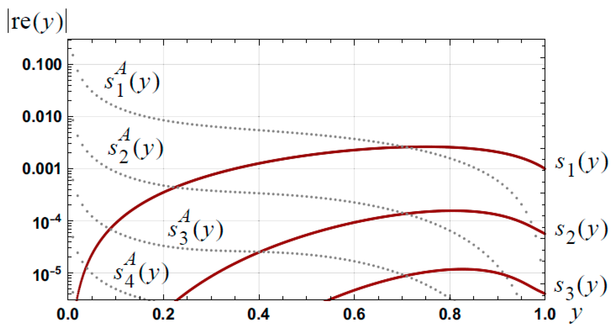
Figure 5.
Graph of the relative error in approximations, of orders 1 to 5, for arcsine and arccosine. The dotted curves are for the approximations and .
Figure 5.
Graph of the relative error in approximations, of orders 1 to 5, for arcsine and arccosine. The dotted curves are for the approximations and .

Figure 6.
Graph of the relative error in approximations, of orders 1 to 5, for arctangent.

Figure 7.
Graph of the relative errors in the approximations, as defined in Theorem 2, to arcsine.

Figure 8.
Graph of the relative errors in the approximations, as defined in Theorem 2, to arccosine.
Figure 8.
Graph of the relative errors in the approximations, as defined in Theorem 2, to arccosine.

Figure 9.
Graph of the relative errors in the approximations, as defined in Theorem 2, to arctangent.
Figure 9.
Graph of the relative errors in the approximations, as defined in Theorem 2, to arctangent.

Figure 10.
Graph of the relative errors in the approximations, as defined in Theorem 3, to arc-sin.

Figure 11.
Graph of
for the case of .

Figure 12.
Graphs of the relative errors in approximations, of orders 1 to 6, for arctangent as defined in Theorem 5.
Figure 12.
Graphs of the relative errors in approximations, of orders 1 to 6, for arctangent as defined in Theorem 5.

Figure 13.
Illustration of upper and lower bounded approximations to arcsine and the two basis points , for two point spline based approximations.
Figure 13.
Illustration of upper and lower bounded approximations to arcsine and the two basis points , for two point spline based approximations.

Figure 14.
Graph of the relative errors in approximations to the square of arcsine as given by Equation (123) (orders 2 to 6) and Equation (124) (orders 2 to 4).
Figure 14.
Graph of the relative errors in approximations to the square of arcsine as given by Equation (123) (orders 2 to 6) and Equation (124) (orders 2 to 4).

Figure 15.
Graph of the relative error in approximations to as defined by for , along with root based approximations of orders .
Figure 15.
Graph of the relative error in approximations to as defined by for , along with root based approximations of orders .

Figure 16.
Graph of the relative errors in the Taylor series (orders one to ten) based approximations for the inverse tangent integral, as given by Equation (138), and the proposed approximations (orders one to four) as specified in Equation (139).
Figure 16.
Graph of the relative errors in the Taylor series (orders one to ten) based approximations for the inverse tangent integral, as given by Equation (138), and the proposed approximations (orders one to four) as specified in Equation (139).

Figure 17.
Graph of the relative errors in the approximations, of orders one to six, as defined by In(y) (Equation (153)).
Figure 17.
Graph of the relative errors in the approximations, of orders one to six, as defined by In(y) (Equation (153)).

Table 1.
Relative error bounds for approximations to r2, arcsine, arccosine and arctangent. The interval [0, 1] is assumed for r2, arcsine and arccosine whilst the interval [0, ∞) is assumed for arctangent.
Table 1.
Relative error bounds for approximations to r2, arcsine, arccosine and arctangent. The interval [0, 1] is assumed for r2, arcsine and arccosine whilst the interval [0, ∞) is assumed for arctangent.
| Order of Approx. | Relative Error Bound: r2 | Relative Error Bound: | Relative Error Bound: |
|---|---|---|---|
| 0 | |||
| 1 | |||
| 2 | |||
| 3 | |||
| 4 | |||
| 5 | |||
| 6 | |||
| 8 | |||
| 10 | |||
| 12 | |||
| 16 |
Table 2.
Relative error bounds, over the interval [0, 1] (arcsine and arccosine) and [0, ∞) (arctangent), associated with the approximations to arcsine, arccosine and arctangent as defined in Theorem 2.
Table 2.
Relative error bounds, over the interval [0, 1] (arcsine and arccosine) and [0, ∞) (arctangent), associated with the approximations to arcsine, arccosine and arctangent as defined in Theorem 2.
| Order of Approx. | Relative Error Bound: | Relative Error Bound: |
|---|---|---|
| 1 | ||
| 2 | ||
| 3 | ||
| 4 | ||
| 5 | ||
| 6 | ||
| 8 | ||
| 10 | ||
| 12 | ||
| 16 |
Table 3.
Relative error bounds associated with the approximations, specified in Theorem 3, for arcsine, arccosine (interval ) and arctangent (interval ).
Table 3.
Relative error bounds associated with the approximations, specified in Theorem 3, for arcsine, arccosine (interval ) and arctangent (interval ).
| Order of Approx. | Relative Error Bound: |
|---|---|
| 0 | 0.145 |
| 1 | 2.63 × 10⁻³ |
| 2 | 1.56 × 10⁻⁴ |
| 3 | 1.18 × 10⁻⁵ |
| 4 | 1.00 × 10⁻⁶ |
| 5 | 9.22 × 10⁻⁸ |
| 6 | 8.91 × 10⁻⁹ |
| 8 | 9.19 × 10⁻¹¹ |
| 10 | 1.03 × 10⁻¹² |
| 12 | 1.23 × 10⁻¹⁴ |
| 16 | 1.95 × 10⁻¹⁸ |
Table 4.
Relative error bounds, associated with the approximations detailed in Theorem 5 and Theorem 6 for arcsine, arccosine and arctangent. The interval is assumed for arcsine and arccosine; the interval for arctangent.
Table 4.
Relative error bounds, associated with the approximations detailed in Theorem 5 and Theorem 6 for arcsine, arccosine and arctangent. The interval is assumed for arcsine and arccosine; the interval for arctangent.
| Order of Spline Approx. | Theorem 5—Relative Error Bounds: | Theorem 6—Relative Error Bound for Arctangent. The Value Assumed for δn,0 is the Second Value Stated in Equation (92). |
|---|---|---|
| 0 | ||
| 1 | ||
| 2 | ||
| 3 | ||
| 4 | ||
| 5 | ||
| 6 | ||
| 8 | ||
| 10 |
Table 5.
Relative error bounds for Newton-Raphson iterative approximations to arcsine and arctangent and based on ,
, and as defined in Theorem 2 and specified by Equations (49) and (50).
Table 5.
Relative error bounds for Newton-Raphson iterative approximations to arcsine and arctangent and based on ,
, and as defined in Theorem 2 and specified by Equations (49) and (50).
| Order of Iteration | Relative Error Bound: | Relative Error Bound: | Relative Error Bound: | Relative Error Bound: |
|---|---|---|---|---|
| 0 | ||||
| 1 | ||||
| 2 | ||||
| 3 | ||||
| 4 | ||||
| 5 |
Table 7.
Relative error bounds, over the interval [0, 1], for the approximations detailed in Theorem 9 for and .
Table 7.
Relative error bounds, over the interval [0, 1], for the approximations detailed in Theorem 9 for and .
| Order, n, of Approx. | Precision: Digits in Roots | Relative Error Bound: k = 1 | Relative Error Bound: k = 2 | Relative Error Bound: k = 3 |
|---|---|---|---|---|
| 2 | 5 | 3.66 × 10⁻⁴ | 7.32 × 10⁻⁴ | 1.10 × 10⁻³ |
| 4 | 8 | 2.48 × 10⁻⁶ | 4.96 × 10⁻⁶ | 7.43 × 10⁻⁶ |
| 6 | 9 | 2.25 × 10⁻⁸ | 4.49 × 10⁻⁸ | 6.74 × 10⁻⁸ |
| 8 | 11 | 2.28 × 10⁻¹⁰ | 4.55 × 10⁻¹⁰ | 6.83 × 10⁻¹⁰ |
| 10 | 13 | 2.93 × 10⁻¹² | 5.85 × 10⁻¹² | 8.78 × 10⁻¹² |
Table 8.
Relative error bounds, over the interval , for Taylor series based approximation, and the approximations specified in Equation (139), for the inverse tangent integral function.
Table 8.
Relative error bounds, over the interval , for Taylor series based approximation, and the approximations specified in Equation (139), for the inverse tangent integral function.
|
Relative Error Bound: Taylor Series | ||
|---|---|---|
| 1 | ||
| 2 | ||
| 3 | ||
| 4 | ||
| 5 | ||
| 6 |
Table 9.
Table of the relative errors associated with the approximations and as defined by Equations (152) and (154).
Table 9.
Table of the relative errors associated with the approximations and as defined by Equations (152) and (154).
| Order of Approx: n | |||
|---|---|---|---|
| 1 | |||
| 2 | |||
| 3 | |||
| 4 | |||
| 6 | |||
| 8 | |||
| 10 |
Table 10.
Approximations for arcsine. The coefficients , and are defined in the associated reference.
Table 10.
Approximations for arcsine. The coefficients , and are defined in the associated reference.
| Reference | Approximation for Arcsine of Order n | Relative Error Bound for [0, 1], n = 4 |
|---|---|---|
| Corollary 1 | ||
| Theorem 2 | ||
| Theorem 3 | ||
| Theorem 5 (Equation (86)) |
Table 11.
Approximations for arctangent. The coefficients , and are defined in the associated reference.
Table 11.
Approximations for arctangent. The coefficients , and are defined in the associated reference.
| Reference | ||
|---|---|---|
| Corollary 1 | ||
| Theorem 2 | ||
| Theorem 3 | ||
| Theorem 5 | ||
| Theorem 6 |
Disclaimer/Publisher’s Note: The statements, opinions and data contained in all publications are solely those of the individual author(s) and contributor(s) and not of MDPI and/or the editor(s). MDPI and/or the editor(s) disclaim responsibility for any injury to people or property resulting from any ideas, methods, instructions or products referred to in the content. |
© 2023 by the author. Licensee MDPI, Basel, Switzerland. This article is an open access article distributed under the terms and conditions of the Creative Commons Attribution (CC BY) license (https://creativecommons.org/licenses/by/4.0/).
Share and Cite
MDPI and ACS Style
Howard, R.M. Radial Based Approximations for Arcsine, Arccosine, Arctangent and Applications. AppliedMath 2023, 3, 343-394. https://doi.org/10.3390/appliedmath3020019
AMA Style
Howard RM. Radial Based Approximations for Arcsine, Arccosine, Arctangent and Applications. AppliedMath. 2023; 3(2):343-394. https://doi.org/10.3390/appliedmath3020019
Chicago/Turabian StyleHoward, Roy M. 2023. "Radial Based Approximations for Arcsine, Arccosine, Arctangent and Applications" AppliedMath 3, no. 2: 343-394. https://doi.org/10.3390/appliedmath3020019