Electricity Price Forecasting via Statistical and Deep Learning Approaches: The German Case

Abstract

Our research involves analyzing the latest models used for electricity price forecasting, which include both traditional inferential statistical methods and newer deep learning techniques. Through our analysis of historical data and the use of multiple weekday dummies, we have proposed an innovative solution for forecasting electricity spot prices. This solution involves breaking down the spot price series into two components: a seasonal trend component and a stochastic component. By utilizing this approach, we are able to provide highly accurate predictions for all considered time frames.

1. Introduction

The study of electricity price forecasting (EPF) [1,2,3,4,5] has attracted increasing attention within European energy markets at least since 1996 as a result of liberalization protocols adopted by the European Authority for Energy. The latter led to an increased complexity of the European electricity market, as a whole, as well as with respect to each single production/consumption of its components.

The most studied aspect of electricity price forecasting concerns short time horizons, i.e., from hours to a day, with the underlying dynamics being different from those of other commodities. Indeed, electricity can not be stored, and a constant balance between generation and consumption is required. Demand, in turn, is subject to hourly, daily, and seasonal fluctuations and is also influenced by the economic activities of the countries involved, political changes, the behavior of weather variables (temperature, solar radiation, wind speed/direction, etc.), and the dynamics of interconnected markets.

Focusing on the German market, starting in 2017, renewable energy sources began to acquire more and more relevance, with an increase of 38.5%, leading to an adjustment in short-term electricity trading because of the implicit volatility due to variation in weather conditions [6]. The latter implied the need to develop models able to simultaneously consider point forecasts, probabilistic forecasts [7], or path forecasts. We first focus on studying electricity prices by applying standard statistical models and then shift our focus to machine learning-based solutions. In recent years, hybrid models have been extensively researched, and there are a number of highly sophisticated and complex hybrid models in the literature. Both daily average and hourly prices are predicted for different time windows. For daily average prices, medium and long time horizons are considered. For hourly prices, medium and short time horizons are considered. The rest of the paper is organized as follows: Section 2 and Section 3 present the statistical models for forecasting and the machine and deep learning models. Section 4 discusses hybrid models and Section 5 contains the analysis of our data and shows the results obtained. Finally, Section 6 discusses the results and possible future work.

2. Benchmark Data and Statistical Models

We focus on forecasting electricity price behavior within the German market with respect to both large time windows (months) and short time windows (days). We implement statistical as well as deep learning models, exploiting German market hourly prices from 2020 and until mid-2022. For the sake of simplicity, we have assumed that the year 2020 is a non-leap year, in order to have all the years with 365 days. It is worth mentioning that our datasets are characterized by not so regular behavior. Indeed, we saw an increasing trend, starting in July 2021 culminating in March 2022, probably incorporating effects due to the Russia–Ukraine conflict. Moreover, we underline how the analyzed years have seen the huge impact of the COVID-19 pandemic as well as an energy crisis that, in Germany, implied supply contracts with delivery in 2023 to be over 1000 EUR per Mw/h and up to 800 EUR per Mw/h in August 2022. Finally, 2022 saw significant changes since German renewable electricity covered 49% of demand during the first six months. In what follows, we denote the price P at time t by $P_t$, then discretize the period of interest–say $[0,T]$–with T positive but finite in regular N, $N\in {\mathbb{N}}^{+}$ and finite sub-intervals with equally spaced extremes $t_i$, $i=1,\dots ,N$, i.e., observations are collected at fixed time (hourly) intervals. We used the most recent prices along considered time windows, dividing the time series into segments with the ‘same’ price level and exploiting algorithms such as K-nearest neighbor (KNN) [8] or the more recent narrowest over threshold (NOT) [9], to select the calibration sample based on similarities with respect to a subset of explanatory variables, leading to a remarkable improvement in forecasting.

As a naive benchmark, we used a method belonging to the class of similar-day techniques: the electricity price forecast for hour h on Tuesday, Wednesday, Thursday, and Friday is set equal to the price for the same hour on the previous day, i.e., ${\widehat{P}}_{d,h}=P_{d-1,h},$ while for hour h on Saturday, Sunday, and Monday, forecasts are set equal to the price for the same hour of the previous week, i.e., ${\widehat{P}}_{d,h}=P_{d-7,h}$.

Statistical Models

Among statistical models usually exploited for time series prediction, let us recall autoregressive moving average (ARMA) along with its extensions and generalized au- toregressive conditional heteroskedastic (GARCH) [10]. For the sake of completeness, let us recall the definitions of autoregressive (AR) and moving average (MA), to then analyze autoregressive moving average and its extensions.

An autoregressive model of order p, indicated as $AR\left(p\right)$, predicts a variable of interest using a linear combination of past values of that variable. This model takes into account the random nature and time correlations of the phenomenon studied, starting with previous prices. The AR model reads:

$$P_t=\alpha +{\varphi }_1{P}_{t-1}+{\varphi }_2{P}_{t-2}+\cdots +{\varphi }_p{P}_{t-p}+{ϵ}_t,$$

(1)

where ${ϵ}_t$ takes into account the randomness component, being modeled by a white noise stochastic process.

A moving average model predicts a variable using a linear combination of past forecast errors: this model considers q previous values of the noise, thus performing a totally different procedure compared to the AR models.We denote by $MA\left(q\right)$ a Moving Average model of order q:

$$P_t=\alpha +{ϵ}_t+{\theta }_1{ϵ}_{t-1}+{\theta }_2{ϵ}_{t-2}+\cdots +{\theta }_q{ϵ}_{t-q},$$

(2)

with ${ϵ}_t$ being defined as above.

The autoregressive moving average model is denoted by $ARMA(p,q)$, where p and q are the coefficients of AR and MA, respectively. In the $ARMA(p,q)$ model, the price $P_t$ is defined as

$$\varphi \left(B\right)P_t=\theta \left(B\right){ϵ}_t,$$

(3)

where B is the backward shift operator, i.e., $B{P}_t=P_{t-1}$. In detail, the $\varphi \left(B\right)$ and $\theta \left(B\right)$ terms are:

$$\varphi \left(B\right)=1-{\varphi }_{1}B-\dots -{\varphi }_p{B}^p\mathrm{and}\theta \left(B\right)=1+{\theta }_{1}B+\dots +{\theta }_q{B}^q,$$

where ${\varphi }_1,\cdots ,{\varphi }_p$ and ${\theta }_1,\cdots ,{\theta }_q$ represent the coefficients of the AR and MA polynomials, while ${ϵ}_t$ can be seen as a collection of independent and identically distributed (i.i.d.) Gaussian random variables, i.e., ${ϵ}_t\sim WN(0,{\sigma }^2)$, hence specifying the white noise component cited before at each time of interest.

Since the ARMA model can be applied only to stationary time series (i.e., time series whose properties do not depend on the time at which the series is observed: time series with trends, or with seasonality, are thus not stationary), we applied unit root tests (ADF, KPSS, and PP); see [11].

The previous point can be overcome by the autoregressive integrated moving average model, ARIMA, introduced in 1976 by Box and Jenkins [12] to consider non-stationary time series by exploiting a differencing technique. The latter allows for removing both trend and seasonality to obtain a stationary time series from data with a period d. First, we have to introduce the $lag-d$ differencing operator ${\nabla }_d$ defined as

$${\nabla }_d{P}_t=P_t-P_{t-d}=(1-B^d)P_t.$$

(4)

The $ARIMA(p,d,q)$ model can be written as:

$$\varphi \left(B\right){\nabla }^d{P}_t=\theta \left(B\right){ϵ}_t,$$

(5)

where p and q are the order for the AR and MA models, respectively. Here d indicates the number of differencing passes at lag d. When the time series is also characterized by seasonality, a standard approach is to use the seasonal autoregressive integrated moving average model, SARIMA, an extension of ARIMA. The $SARIMA(p,d,q)\times {(P,D,Q)}_s$ model is defined as

$$\varphi \left(B\right)\mathsf{\Phi }\left(B^s\right){\nabla }^d{\nabla }_s^D{P}_t=\theta \left(B\right)\mathsf{\Theta }\left(B^s\right){ϵ}_t,$$

(6)

where $(p,d,q)$ refers to the non-seasonal component, while $(P,D,Q)$ refers to the seasonal ones, and s indicates the number of observations in a season. Since every SARIMA model can be transformed into an ARMA model using the variable ${\tilde{P}}_t={\nabla }^d{\nabla }_s^D{P}_t$, prediction is accomplished in two steps: model identification and estimation of the parameters; see Section 5.3.2.

Next, we introduce an autoregressive model for hourly price prediction where dummies are considered. The model uses the ARX model as a starting point but does not include exogenous variables:

$$\begin{array}{cc}\hfill P_{d,h}& ={\beta }_1{P}_{d-1,h}+{\beta }_2{P}_{d-2,h}+{\beta }_3{P}_{d-7,h}+{\beta }_4{P}_{d-1,24}+{\beta }_5{P}_{d-1}^{max}+{\beta }_6{P}_{d-1}^{min}+\sum _{j=1}^7{\beta }_{h,j+8}{D}_j+{ϵ}_{d,h},\hfill \end{array}$$

(7)

where $P_{d-1,h}$, $P_{d-2,h}$, and $P_{d-7,h}$ account for the autoregressive effects corresponding to prices from the same hour h of the previous day, two days before and a week before. The coefficient $P_{d-1,24}$ is the last known price at the time when the prediction is made, thus providing information about the end-of-day price level. Coefficients $P_{d-1}^{min}$ and $P_{d-1}^{max}$ are the previous day’s minimum and maximum prices, respectively. Lastly, $D_1,\cdots ,D_7$ are weekday dummies, and ${ϵ}_{d,h}$ is the noise term, which is assumed to be i.i.d. and with finite variance; then we estimate the ${\beta }_i$’s using least absolute shrinkage and selection operator.

3. Machine Learning Based Models

For the sake of completeness, in what follows we recall basics about extreme gradient boosting and neural network models.

3.1. The XGBoost Model

The extreme gradient boosting (XGBoost) improves gradient booster performances by considering new trees correcting the errors of those trees that are already part of the model. Trees are added until no further improvements can be made to the model, hence implementing a walk forward validation [13] scheme. In particular, we used the XGBoost library [14]. Given a training set ${\left\{(x_t,p_i)\right\}}_{i=1}^N$, a differentiable loss function $L(p,F(x\left)\right)$, a number of weak learners M, and a learning rate $\alpha$ [13], the algorithm is defined as follow:

• Initialization of the model with a constant value:

  $${\widehat{f}}_{\left(0\right)}\left(x\right)=arg\underset{\theta }{min}\sum _{i=1}^{N}L(p_i,\theta ).$$
• For $m=1,\cdots M$:

  (a)

  Compute the gradients and Hessians:

  $${\widehat{g}}_m\left(x_i\right)={\left[\frac{\partial L(p_i,f\left(x_i\right))}{\partial f\left(x_i\right)}\right]}_{f\left(x\right)={\widehat{f}}_{(m-1)}\left(x\right)},{\widehat{h}}_m\left(x_i\right)={\left[\frac{{\partial }^{2}L(p_i,f\left(x_i\right))}{\partial f{\left(x_i\right)}^2}\right]}_{f\left(x\right)={\widehat{f}}_{(m-1)}\left(x\right)}.$$

  (b)

  Fit a base learner using the training dataset ${\left\{x_i,-\frac{{\widehat{g}}_m\left(x_i\right)}{{\widehat{h}}_m\left(x_i\right)}\right\}}_{i=1}^N$

  by solving the optimization problem below:

  $${\widehat{\varphi }}_m=arg\underset{\varphi \in \mathsf{\Phi }}{min}\sum _{i=1}^N\frac{1}{2}{\widehat{h}}_m\left(x_i\right){\left[-\frac{{\widehat{g}}_m\left(x_i\right)}{{\widehat{h}}_m\left(x_i\right)}-\varphi \left(x_i\right)\right]}^2,{\widehat{f}}_m\left(x\right)=\alpha {\widehat{\varphi }}_m\left(x\right).$$

  (c)

  Update the model ${\widehat{f}}_{\left(m\right)}\left(x\right)={\widehat{f}}_{(m-1)}\left(x\right)+{\widehat{f}}_m\left(x\right)$.

• Output: $\widehat{f}\left(x\right)={\widehat{f}}_{\left(M\right)}\left(x\right)={\displaystyle \sum _{m=0}^M}{\widehat{f}}_m\left(x\right)$.

3.2. Neural Network Models

Since the mid-2010s, research on EPF shifted to consider an increasing number of inputs as, e.g., in deep learning models. The latter has been made possible by augmented computational capacities (mainly based on GPUs) at lower costs, also exploiting cloud solutions. As a result, it has been possible to gain better representations of hidden data while maintaining reasonable work times. Neural networks can be equipped to provide anything from a single-valued forecast to a complete interval of possible values.

The first neural networks used for electricity price forecasting were mainly simple ones with one hidden layer such as multilayer perceptron (MLP), radial basis function (RBF) networks, or at most very simple recurrent neural networks. The most common MLP is described as follows: every neuron in the previous layer is fully connected to every neuron in the next layer. In the EPF literature, the input is the past energy load, and the output is the future energy load.

The deep neural network (DNN) is the natural extension of the traditional MLP using multiple hidden layers. Here, our DNN is a deep feedforward neural network [15] with 4 layers within the multivariate framework that exploits the Adam optimizer. Let us underline that the variables defining a DNN with two hidden layers are: the input vector $\mathbf{X}={[x_1,\cdots ,x_n]}^{\top }$, the vector of day-ahead prices we want to predict $\mathit{P}={[p_1,\cdots ,p_{24}]}^{\top }$, and the number of hidden layers of neurons $n_1$, $n_2$.

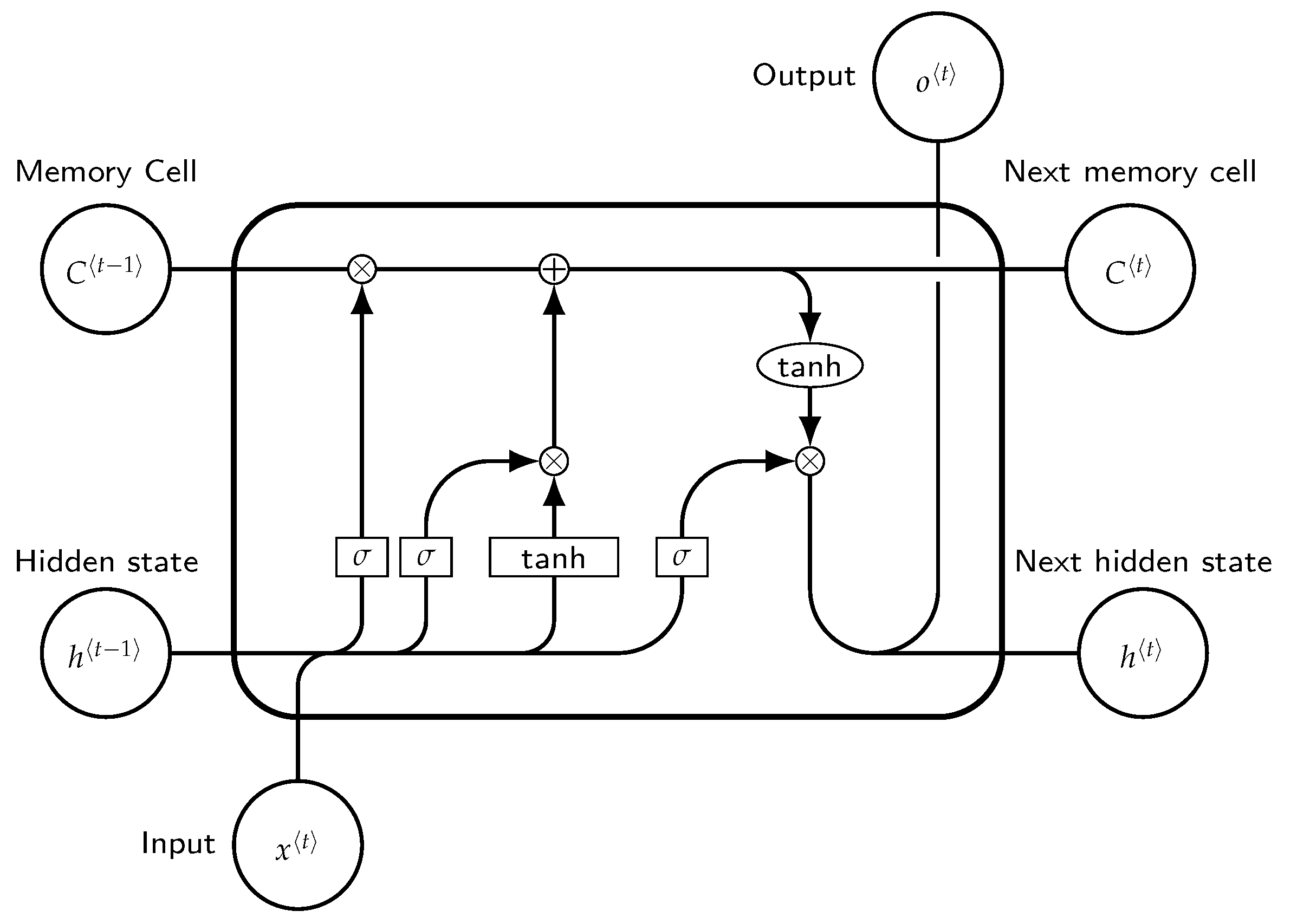
Recurrent neural networks (RNN) are a specialized class of neural networks allowing cyclical connections. Their structure allows for recording past information that can then be used to forecast future values. It is worth mentioning that RNNs only take into account inputs at time $t-1$, hence facing the long-term dependencies problem that can be tackled by long short-term memorys, introduced by Hochreiter and Schmidhuber in 1997 [16]. Long short-term memory (LSTM) neural networks are special variants of RNNs, in which information can be stored, updated, or forgotten by a choice of the state of the cell. This allows such NNs to use large input spaces and understand long-term dependencies. The computational graph of LSTMs contains four basic elements: input gate, forget gate, output gate cell, and state output. Gate operations are performed in the cell memory state and are of the following types: reading, writing, and erasing.

Defining as $x_t$ the input value recorded at time t and by $h_t$, the associated LSTM output, the main steps of this particular neural network solution read as follows:

• Decide which information is going to be removed from the cell state exploiting the sigmoid layer, also called forget gate layer, which considers $x_t$ and $h_{t-1}$, and then returns a value between 0 and 1 for each value in the cell state $C_{t-1}$.
• Decide which new information will be stored in the cell state. This step is divided into two substeps:
  • Use an input gate layer implemented by a sigmoid layer to decide which values will be updated, $i_t=\sigma (W_i\times [h_{t-1},x_t]+b_i)$;
  • Use a tanh layer to provide a vector of new candidate values ${\tilde{C}}_t=tanh(W_C\times \left[h_{t-1,x_t}\right]+b_C)$ that can be added to the state.
  As a result, the old cell state $C_{t-1}$ is updated with $C_t=f_t·C_{t-1}+i_t·{\tilde{C}}_t$, where $f_t·C_{t-1}$ indicates what we have already chosen to forget, and the other term indicates the new candidates.
• The output will be defined by a filtered version of the cell state, via a sigmoid layer deciding which parts will be included in the output $o_t=\sigma (W_o·\left[h_{t-1,x_t}\right]+b_o)$. Then, a tanh is carried out, which is itself multiplied by the output of the sigmoid gate $h_t=o_t·tanh\left(C_t\right)$.

The schematic of such an LSTM is shown in Figure 1.

Another NN that can be used to predict day-ahead prices is the convolutional neural network (CNN), which uses the concept of weight sharing and provides better accuracy in highly non-linear problems. The inputs are divided between those modeling sequential past data ${\mathbf{X}}_{\mathbf{S}}={[x_{S_1},\cdots ,x_{S_N}]}^{\top }$ and those modeling information about next 24 h day-ahead ${\mathbf{X}}_{\mathbf{F}}={[x_{F_1},\cdots ,x_{F_N}]}^{\top }$. With the previous two inputs, the model uses two parallel CNNs to model the electricity price behavior. In particular, the convolution process starts with inputs transformed into the feature maps, then continues according to the pooling process wherein the feature map of the convolution layer is sampled to reduce its dimension. After both networks perform a series of convolution and pooling operations, we have a fully connected layer that models the day-ahead prices $\mathit{P}$.

4. Hybrid Models

In this section, we discuss more modern hybrid models. These models are extremely complex frameworks that consist of a number of algorithms, including for decomposing data, selecting features, clustering data, using one or more forecasting models, and using heuristic optimization algorithms to estimate either the models or their hyperparameters. While these models have performed better than models based on traditional statistics or machine learning (see [17]), determining the best model is impossible for a number of other reasons. First, they have not been compared in the literature to sophisticated techniques such as LEAR or DNN. Therefore, it is impossible to determine the exact effect of each algorithm.

5. Data Analysis

We implemented the above-mentioned models considering hourly electricity prices in Germany ranging from 2020 to mid-2022 and provided a forecast exploiting both daily average and hourly prices on different time windows. Concerning daily average prices, we first carried out a long-term forecast taking holidays into account. The latter could be useful in view of investment planning; e.g., when dealing with mid- to long-term power plant energy demand programming. See, e.g., [18].

The accuracy of a forecast model is defined considering realized errors, e.g., analyzing mean absolute percentage error, mean absolute deviation, and median relative absolute error. For day-ahead forecasting, those errors are not a good choice, since the economic decision might lead to economic benefits or damage, depending on the forecast precision. Rather, according to the literature, a better choice is represented by quadratic errors, i.e., $L_2$, such as the mean square error (MSE)

$$MSE=\frac{1}{n}\sum _{t=1}^n{({\widehat{P}}_t-P_t)}^2$$

or the related root mean square error (RMSE), defined as: $RMSE=\sqrt{MSE}$.

5.1. Naive Benchmark Results

We first show results obtained from the naive benchmark; see Section 2.

5.1.1. Daily Average Price

In the analysis of average daily prices, hours were not taken into account. That is, the forecast is equivalent to the price of the previous day except for Saturday, Sunday, and Monday, which are considered to be those of the previous week. These results, in

Table 1. RMSE of naive benchmark on different training and test periods for daily average prices.

Naive Benchmark
Training Period	Test Period	RMSE
2020	2021	91.0102
2020–2021	2022	150.4029
two weeks in 2020	two weeks in 2021	56.0675

, show that this model does not accurately identify future prices; in fact, the errors are considerable.

5.1.2. Hourly Daily Price

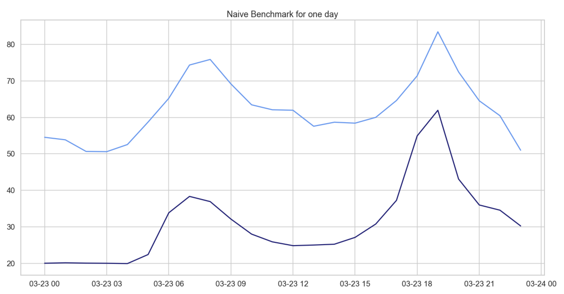
In what follows, we provide the errors characterizing the naive benchmark applied to the prediction of daily hourly prices over different time windows. From

Table 2. RMSE of the naive benchmark model on different training and test periods for daily hourly prices.

Naive Benchmark
Training Period	Test Period	RMSE
one month in 2020	one month in 2021	123.8230
one week in 2020	one week in 2021	51.5851
one day in 2020	one day in 2021	31.6256

, showing the RMSEs, we can deduce that, as in the previous case concerning daily average prices, this model does not perform well on our data. Indeed, naive benchmark predictions are far in terms of values from the current price, but as we show in Figure 2, the behavior is predicted very accurately, due to the fact that the years 2020 and 2021 had similar daily behavior during the first months of the year.

5.2. SARIMA

In what follows, we consider the SARIMA model, which takes into account atheseasonality component characterizing our time series. We first consider the autocorrelation function (ACF) and the partial autocorrelation function (PACF), in order to focus on parameters q and p, respectively. To identify m, it is sufficient to analyze the time series provided. It is crucial to note that the choice of m affects the seasonal parameters $P,D,$ and Q. Values of parameters d and D can be determined by a unit root test, which is ADF in our study, or by looking at the rolling mean and the rolling standard deviation.

5.2.1. Daily Average Price

In the context of daily average prices of electricity, the seasonality magnitude is defined as $m=7$, since we observed periodic weekly behavior. The parameters of the model SARIMA, for the forecasts of the daily average prices, were chosen, observing ACF and PACF plots and using the library pmdarima.

We can rely on these results, as we checked the p-value of each individual parameter that is less than 0.05, hence less statistically significant. Analogously, we checked the p-value of the Ljung–Box test, which suggests not rejecting the null hypothesis. Therefore, the residuals are independently distributed, hence defining white noise.

In

Table 3. RMSE of the SARIMA model of 2020–2021 for testing mid-2022 for the daily average prices.

SARIMA (2, 0, 2) × (0, 1, 1)${}_7$
Training Period	RMSE
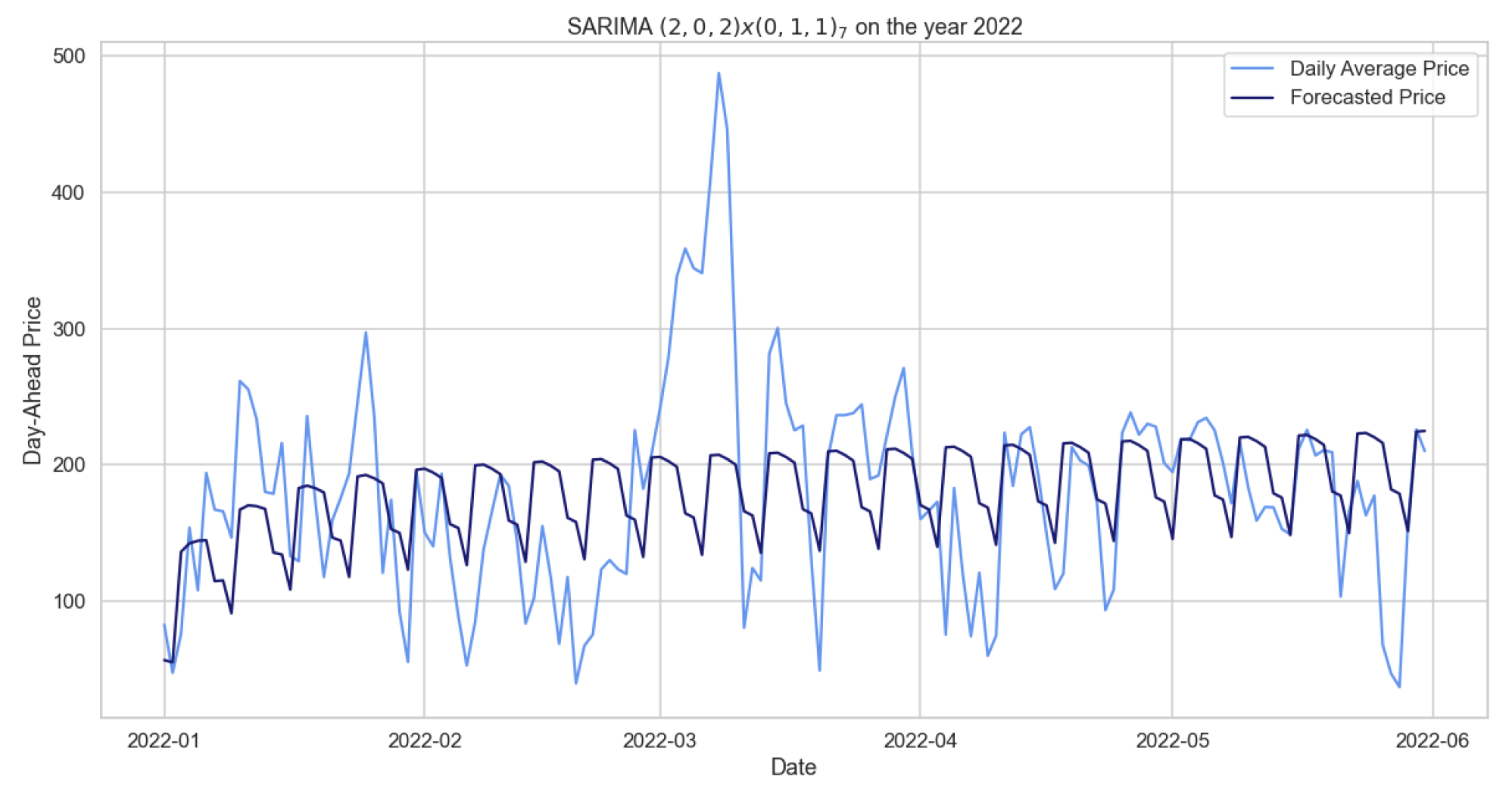
2020–2021	77.6600

, we observe errors obtained from the SARIMA model trained on data from 2020 to 2021 to predict mid-2022; however, they are much lower than the ones for the model previously observed. Additionally, we can consider the results obtained valid because the p-value of the Ljung–Box test is 0.92, which is much greater than 0.05; therefore, the residuals are independent.

Although we can consider these results as satisfying the model’s assumptions, and although they fit better than the previous model, we observe in Figure 3 that SARIMA predicts regular and periodic behavior that is not reflected in our data. Is also interesting to observe a significant peak in March, an unexpected datum probably due to the war between Russia and Ukraine that started one week before. As for the other SARIMA models,

Table 4. RMSE of the SARIMA model trained on different time windows for testing two weeks.

RMSE of Two Weeks of Testing in 2021
Training Period	$\mathit{SARIMA}(\mathit{p},\mathit{d},\mathit{q})\times {(\mathit{P},\mathit{D},\mathit{Q})}_{\mathbf{7}}$	RMSE
2020	$\mathit{SARIMA}(1,1,2)\times {(1,0,2)}_7$	23.3416
Spring–Summer	$\mathit{SARIMA}(2,1,1)\times {(0,1,1)}_7$	17.1818
Autumn–Winter	$\mathit{SARIMA}(1,1,3)\times {(4,1,3)}_7$	12.2135

provides errors obtained with respect to different time windows used as training periods, while maintaining two weeks as the set test period.

In

Table 5. The p-values of the Ljung–Box test for the SARIMA model for 2 weeks of testing.

Ljung–Box Test
Training Period	$\mathit{p}$-Value	Null Hypothesis
2020	0.93	not rejected
Spring–Summer	0.87	not rejected
Autumn–Winter	0.69	not rejected

, we show the p-values for the Ljung–Box test, which allows us to state that the three models are reliable. In Figure 4, we observe the forecast made by the SARIMA model for a fortnight. The model predicts a more regular behavior than the current one and fails to predict peaks.

5.2.2. Hourly Daily Price

We considered daily hourly prices, starting by predicting a month using different time windows, then predicting a whole week as well as a single day exploiting the same time windows. The SARIMA models explained above were tested performing the Ljung–Box test as shown in

Table 6. The p-values of the Ljung–Box test for the SARIMA model of a one-month test.

Ljung–Box Test
Training Period	$\mathit{p}$-Value	Null Hypothesis
2020	0.33	not rejected
Spring–Summer	0.92	not rejected
Autumn–Winter	0.96	not rejected

. In

Table 7. RMSE of the SARIMA model of different time windows for testing one month in 2021.

RMSE of One Month of Testing in 2021
Training Period	$\mathit{SARIMA}(\mathit{p},\mathit{d},\mathit{q})\times {(\mathit{P},\mathit{D},\mathit{Q})}_{24}$	RMSE
2020	$\mathit{SARIMA}(2,1,1)\times {(2,1,0)}_{24}$	118.8870
Spring–Summer	$\mathit{SARIMA}(2,0,2)\times {(2,1,0)}_{24}$	107.9992
Autumn–Winter	$\mathit{SARIMA}(2,0,0)\times {(2,1,0)}_{24}$	110.7636

and

Table 8. RMSE of the SARIMA model of different time windows for testing one week.

RMSE of One Week of Testing in 2021
Training Period	SARIMA (p, d, q) × (P, D, Q)${}_{\mathbf{24}}$	RMSE
2020	$\mathit{SARIMA}(2,1,0)\times {(2,1,0)}_{24}$	41.7355
Spring–Summer	$SARIMA(2,0,2)\times {(2,1,0)}_{24}$	19.6915
Autumn–Winter	$SARIMA(2,0,0)\times {(2,1,0)}_{24}$	16.5124

, we see the results obtained from SARIMA models to predict a month or a week. In the case of the autumn–winter training set, it turns out to be a good prediction; in fact, it is the lowest RMSE obtained in these SARIMAs.

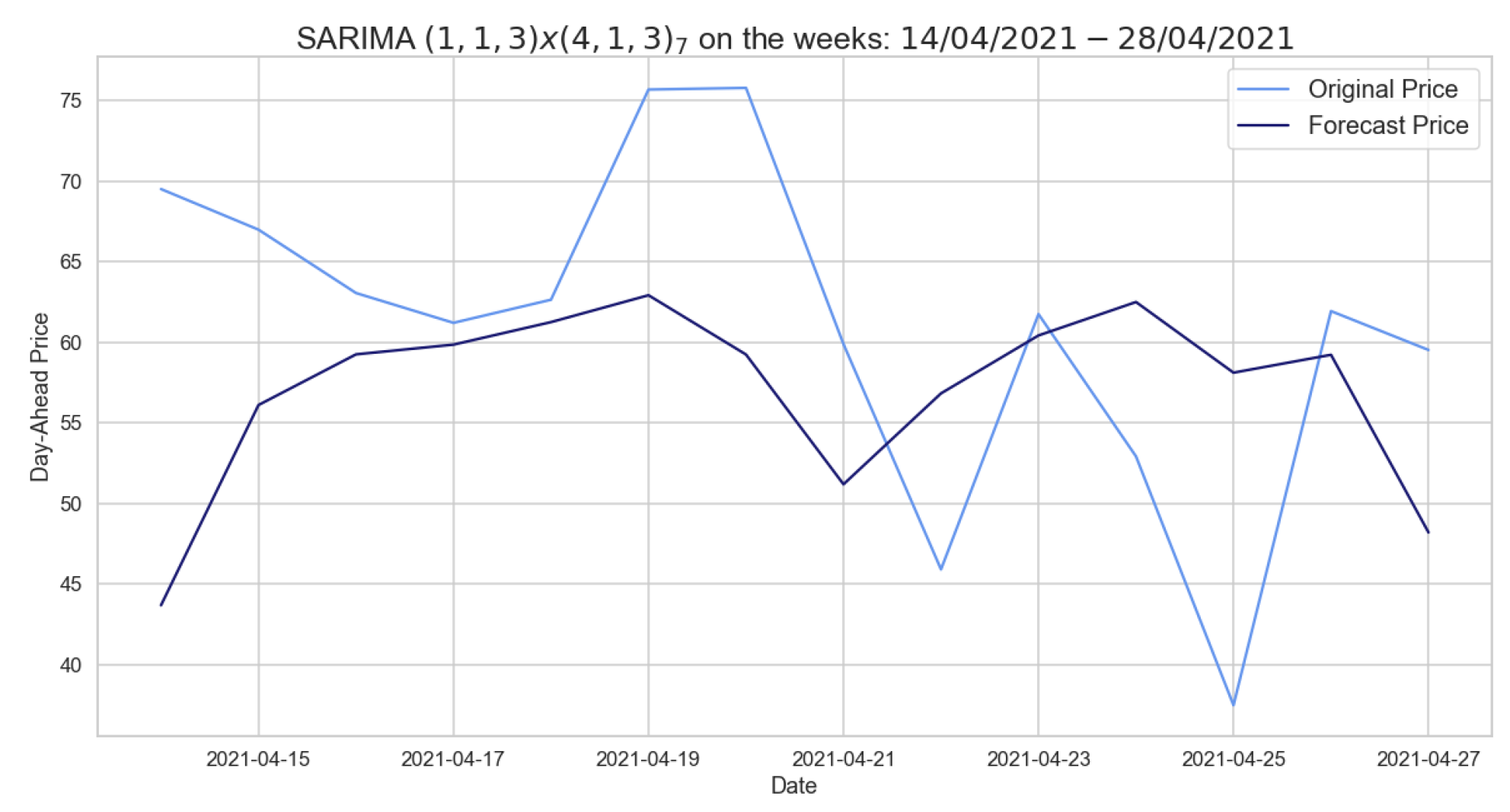
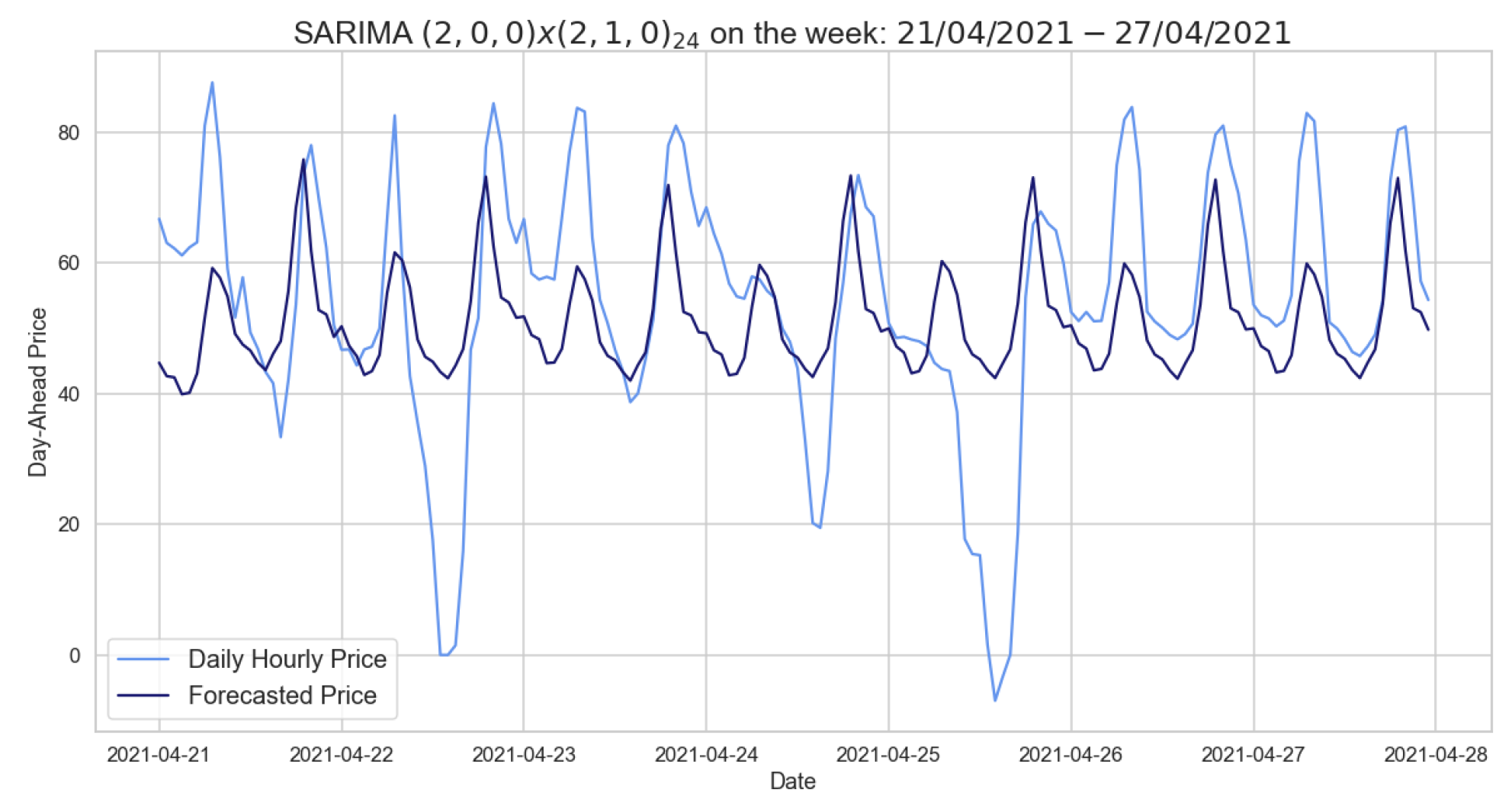
Figure 5 presents the forecasts provided by the SARIMA model, using autumn–winter as training set and testing one week in 2021, which predicts positive peaks quite well while not detecting prices approaching zero.

Table 9. RMSE of the SARIMA model of different time windows for testing one day for the hourly prices.

RMSE of One Day of Testing in 2021
Training Period	$\mathit{SARIMA}(\mathit{p},\mathit{d},\mathit{q})\times {(\mathit{P},\mathit{D},\mathit{Q})}_{\mathbf{24}}$	RMSE
2020	$SARIMA(2,1,0)\times {(2,1,0)}_{24}$	7.8986
Spring–Summer	$SARIMA(2,0,2)\times {(2,1,0)}_{24}$	16.9000
Autumn–Winter	$SARIMA(2,0,0)\times {(2,1,0)}_{24}$	12.1786

shows the errors obtained by SARIMA models for one day using different time series as training sets. For these models, p-values were measured for the Ljung–Box test, all of which allow us to state the models considered are defined by independent residuals.

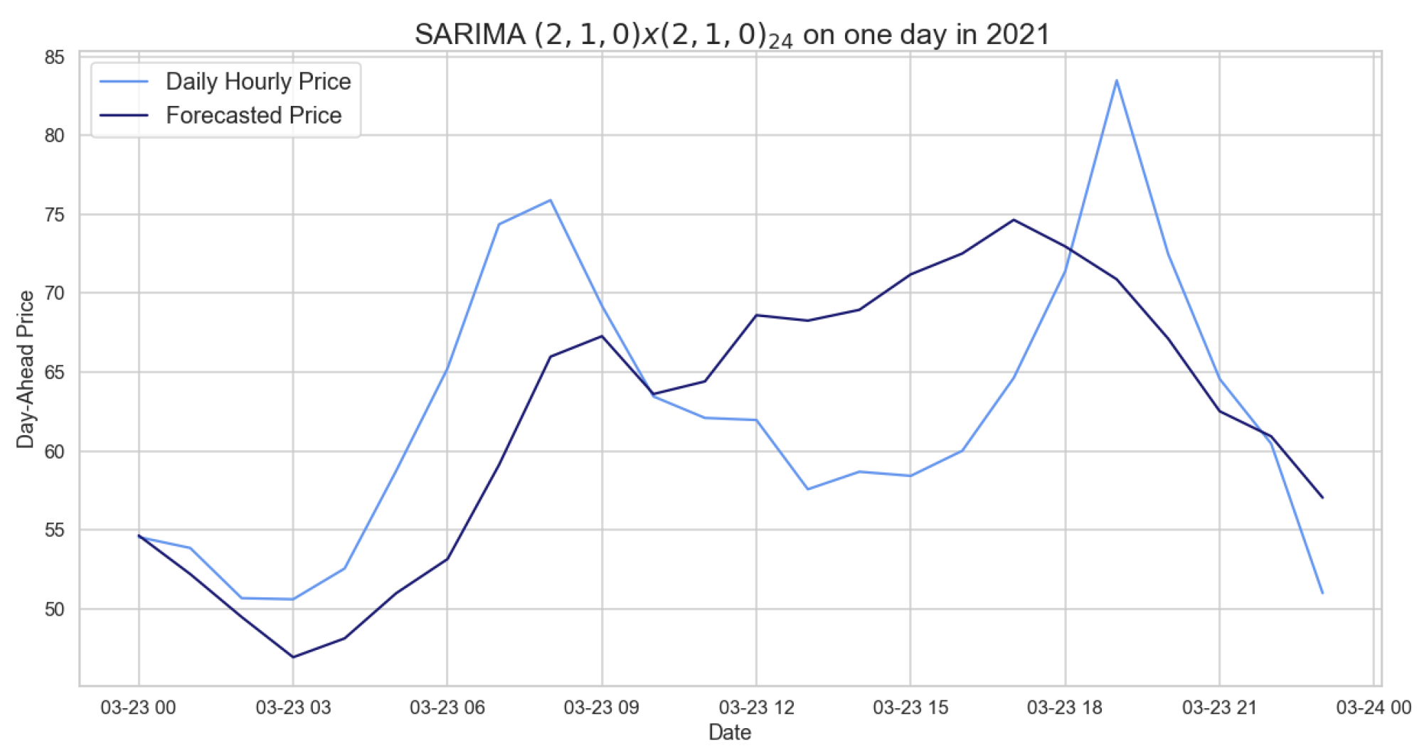
Figure 6 displays the 24 h period forecast provided by the previously stated model, showing that it does not obtain precise results since, e.g., it is able to predict only one peak whereas our time (hourly) series are characterized by two peaks. It follows that the SARIMA model performs better than the naive benchmark on both daily average and hourly prices, even if it is not accurate as shown by the RMSEs.

5.3. Deseasonalization

In this section, we deseasonalize our time series, applying the wavelet decomposition. Using the time series with a seasonal adjustment clearly improves the accuracy obtained in both simple autoregression and structured models with automated variable selection via LASSO. Moreover, such seasonal decomposition has also turned out to work well for deep learning-based models for both point forecasts and probabilistic forecasts.

Seasonal decomposition refers to the representation of a signal as a sum and/or product of a periodic component; the remaining variability is typically described by the action of a stochastic process that could allow for jumps. We referred to the wavelets approach because, after numerical implementation, the RMSEs obtained from forecasts made with the same models on time series with a seasonal adjustment done with the HP filter are similar.

5.3.1. Wavelet Decomposition

Wavelet transformation is based on a series of functions called wavelets, each defined with respect to a different scale. A wavelet family consists of pairs composed by a father, also called scaling function, and a mother, respectively indicated with $\varphi$ and $\psi$. In detail, the father wavelet is representing the low frequency smooth components, while the mother captures the higher frequency components. Every wavelet family is defined with an order, indicating the number of vanishing moments related to the approximation order and smoothness of the wavelet.

Additionally, there are two assumptions of the wavelet: finite energy and zero mean. Finite energy means that it is localized in time and frequency; it is integrable, and the inner product between the wavelet and the signal always exists. The admissibility condition implies a wavelet to have zero mean in the time domain, and a zero at zero frequency in the time domain. This is necessary to ensure that it is integratable and that the inverse of the wavelet transform can also be calculated.

We decided to use the Daubechies family of order 24 (see Weron [19] in the MATLAB code ‘deseasonalize.m’) with smoothing level k from 6 to 14, according to [20], since the resulting specification is sufficiently smooth for our datasets. To perform the wavelet decomposition in Python, the (open source) PyWavelets library, particularly the functions ‘wavedec’, ‘waverec’, and ‘threshold’ [21], has been exploited.

In wavelet smoothing, the time series is decomposed using the discrete wavelet transform into a sum of approximation series capturing the general trend, $S_J$, and a number of detailed series $D_J$ representing the high frequency components: $S_J+D_J+D_{J-1}+\cdots +D_1$, where J is the smoothing level,

$$S_J=\sum _k{s}_{J,k}{\varphi }_{J,k}\left(t\right)\mathrm{and}{D}_j=\sum _k{d}_{j,k}{\psi }_{j,k}\left(t\right).$$

The terms $s_{J,k},d_{J,k},d_{J-1,k},\cdots ,d_{1,k}$ indicate the wavelet transform coefficients that measure the contribution of the corresponding wavelet function to the approximation sum. At the coarsest scale, the LTSC term can be approximated by $S_J$ and more precisely by $S_{J-1}=S_J+D_J$. At each step, we obtain a better estimate of the original signal by adding a mother wavelet $D_j$ of a lower scale $j=J_1,J_2,\cdots$. The reconstruction process can always be interrupted, especially when we reach the desired accuracy, see Figure 7 for an illustration.

Daily Average Price

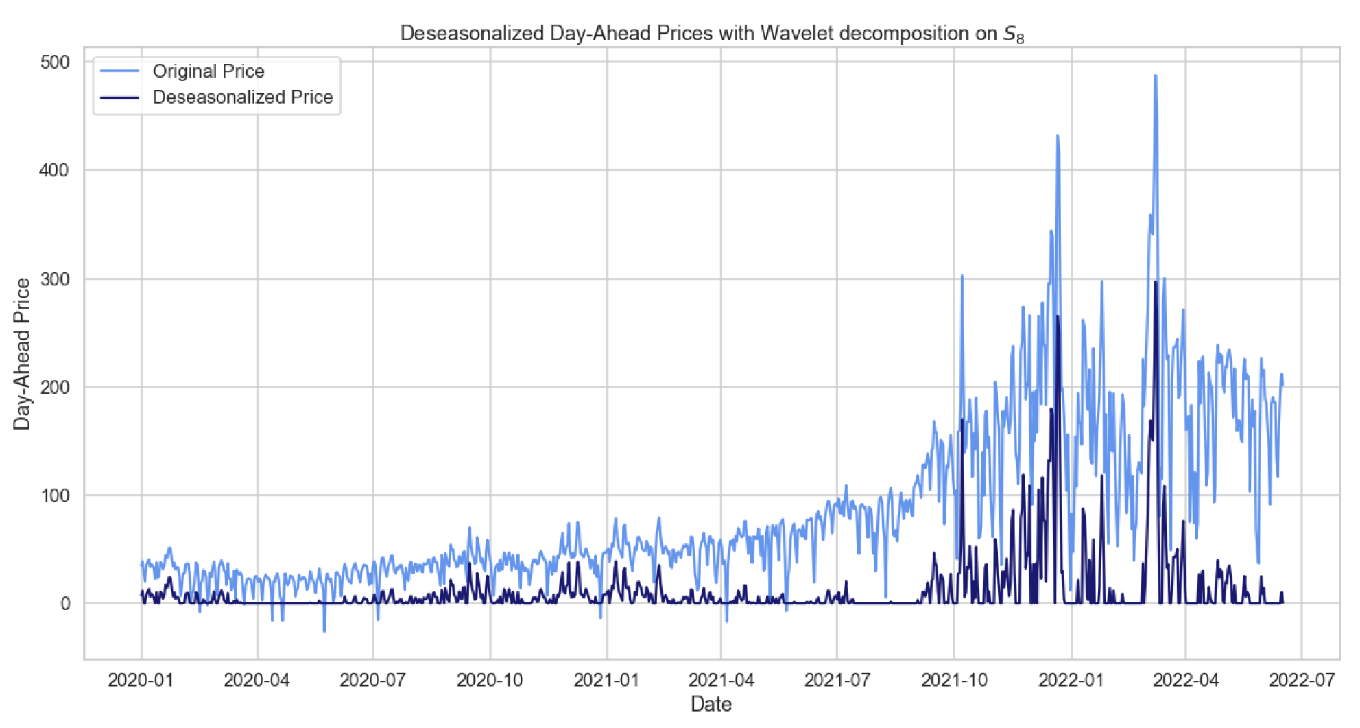
In Figure 8, we observe the daily average prices after removing the long trend seasonal component (LTSC) and after replacing negative values with null prices; see also ‘deseasonalized.m’ MATLAB code [19]. The seasonal adjustment shown below was obtained with the wavelet family ‘db24’ on the wavelet $S_8$.

Hourly Daily Price

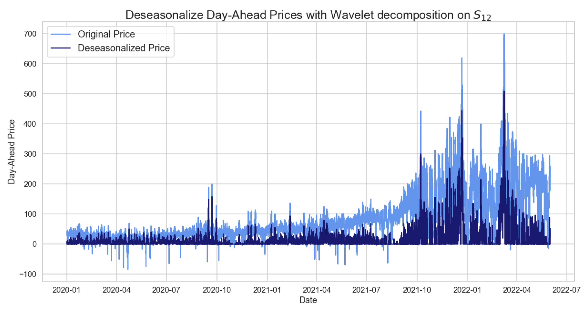
For hourly prices, the LTSC decomposition is done with the same MATLAB code used for daily average prices and is performed on the same wavelet family ‘db24’ using the wavelet $S_{12}$; see Figure 9.

5.3.2. Box–Jenkins Model

The Box and Jenkins approach [22], ARIMA, consists of the following steps: model identification, parameter estimation, estimate the parameters for the model, and model diagnostics [23].

Model Identification

Since ARMA requires stationarity, the standard Box and Jenkins approach suggests both a short and a seasonal differentiation to obtain stationarity of the mean, then performing a logarithmic/power transformation to achieve stationarity in the variance. Analogously, when dealing with seasonal components, we can consider seasonal multiplicative models coupled, when necessary, with long-term differencing to achieve mean stationarity; see, e.g.,  [12].

Parameter Estimation

Dealing with a stationary and deseasonalized time series, we can move forward applying ARMA, hence choosing the order of the parameters p and q, by exploiting autocorrelation function and partial autocorrelation function plots. They, respectively, show correlations in an observation with lag values, a summary of correlations between observations and lag values that are not accounted for by prior lagged observations. Model accuracy is provided by the following criteria:

• Akaike Information Criteria (AIC): goodness-of-fit measure of an estimated statistical model, $AIC=-2log\left(\mathcal{L}\right)+2(p+q+1)$.
• Bayesian Information Criteria (BIC): estimate of the Bayes factor for two competing models $BIC=-2log\left(\mathcal{L}\right)+log\left(N\right)(p+q+1)$.

$\mathcal{L}$ indicates the maximum likelihood function, while N is the number of observations. Hence, the model providing the minor information criteria (IC) is the one to choose, since it identifies both the goodness of the fit and the number of parameters; see, e.g.,  [24,25].

Model Estimation

To estimate the coefficients of the previously chosen $ARMA(p,q)$ model, we can use criteria such as maximum likelihood estimation and least squares estimation.

Model Diagnostic

The last step of the Box–Jenkins methodology concerns a diagnostic check to verify that the model is adequate. Box–Pierce and Ljung–Box tests are used to check the correlation of the residuals.

• The Box–Pierce test is defined as

  $$Q\left(k\right)=N\sum _{i=1}^k{r}_i^2,$$

  where N represents the number of observations, k is the length of coefficients to test autocorrelation, and $r_i$ is the autocorrelation coefficient for lag i.
  The null hypothesis of the Box–Pierce test reads
  $H_0$: none of the autocorrelation coefficients up to lag k is different from zero,
  i.e., the residuals are independently distributed (i.e., white noise), and the model is adequate.
• The Ljung–Box statistics follows this formula:

  $$Q^{*}\left(k\right)=N(N+2)\sum _{i=1}^k\frac{r_i^2}{(N-i)},$$

  where the variables are the same as the Box–Pierce test and the null hypothesis is too.

Daily Average Price

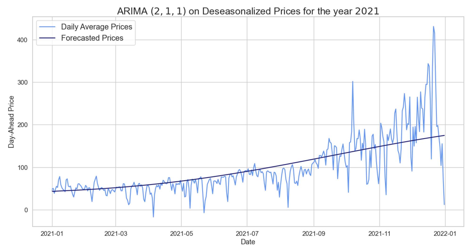
We continue the analysis with statistical models such as ARIMA on the deseasonalized time series. Applying the Box–Jenkins model, we obtained parameters $p=2$, $d=1$, and $q=1$, using the ACF, PACF, and AIC as information criteria. In particular, $d=1$ indicates the non-stationarity of our time series, see Equation (4), and therefore it must be differentiated with $lag=1$ to be stationary.

Additionally, the Ljung–Box test was carried out showing a p-value of 0.83, so we can not reject the null hypothesis. That is, the residuals are independently distributed, and we can consider the results obtained by the model valid.

Table 10. RMSE of the ARIMA model of 2020 for testing 2021 on the daily average deseasonalized prices.

ARIMA$(2,1,1)$
Training Period	RMSE
2020	43.4172

shows the RMSE of the ARIMA model trained on 2020 in order to predict 2021. We observe a clear improvement of the RMSE compared to what is seen in

Table 11. RMSE of the SARIMA model of 2020 for testing 2021 for the daily average prices.

SARIMA (3, 1, 3) × (1, 1, 1)${}_7$
Training Period	RMSE
2020	85.3509

with SARIMA. However, although the RMSE is not large, this is not a result of the model’s ability but only of the seasonal adjustment of the LTSC component, as clearly observed in Figure 10.

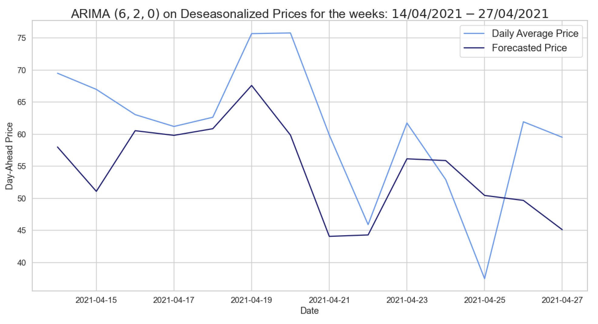
In the same way, we evaluated and obtained the ARIMA’s hyperparameters using the years 2020 and 2021 as the training set and testing mid-2022, as shown in

Table 12. RMSE of ARIMA on 2020–2021 for testing mid-2022 on daily average deseasonalized prices.

ARIMA $(7,1,1)$
Training Period	RMSE
2020–2021	77.6933

. However, this model, in contrast to the previous one, does not perform better than the SARIMA on the same training and test sets. The latest models are designed to forecast two weeks starting from the daily average deseasonalized time series on different time windows. The results of these models are shown in

Table 13. RMSE of the ARIMA model for testing two weeks on daily average deseasonalized prices.

RMSE of Two Weeks of Testing in 2021
Training Period	$ARIMA(\mathit{p},\mathit{d},\mathit{q})$	RMSE
2020	$ARIMA(2,1,1)$	11.1749
Spring–Summer	$ARIMA(6,2,0)$	10.4634
Autumn–Winter	$ARIMA(6,1,6)$	11.2119

and 

Table 14. The p-values of the Ljung–Box test for the ARIMA model on a two-week test.

Ljung–Box Test on a Two-Weeks Test
Training Period	$\mathit{p}$-Value	Null Hypothesis
2020	0.83	not rejected
Spring–Summer	0.24	not rejected
Autumn–Winter	0.95	not rejected

.

The RMSEs are lower than those obtained from the SARIMA model (see Table 4), that was trained on the same training and test sets. Figure 11 shows that the model can predict quite well the weekly behavior. This ARIMA model predicts the two upper peaks quite accurately.

Hourly Daily Price

Let us now consider the hourly prices from which we removed the LTSC component with wavelet decomposition on the wavelet $S_{12}$. After observing plots concerning ACF and PACF and after ascertaining the stationarity of our time series using the ADF test, we obtain the hyperparameters for the different time windows presented in

Table 15. RMSE of the ARIMA model on different training sets for testing one month on the hourly deseasonalized prices.

RMSE of One Month of Testing in 2021
Training Period	$ARIMA(\mathit{p},\mathit{d},\mathit{q})$	RMSE
2020	$ARIMA(4,0,1)$	71.1059
Spring–Summer	$ARIMA(2,0,1)$	71.0840
Autumn–Winter	$ARIMA(7,0,3)$	71.3371

. Before evaluating the errors, we check the reliability of the models using the Ljung–Box test in 

Table 16. The p-values of the Ljung–Box test for the ARIMA models on a one-month test.

Ljung–Box Test on One Month of Test
Training Period	$\mathit{p}$-Value	Null Hypothesis
2020	0.97	not rejected
Spring–Summer	0.99	not rejected
Autumn–Winter	1	not rejected

.

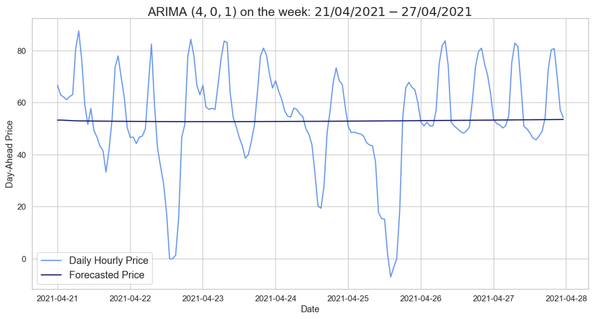
Having checked the models’ reliability, we can state that ARIMA on the seasonally adjusted hourly prices performs better than both the SARIMA and the naive benchmark model.

Table 17. RMSE of the ARIMA model on different training sets for testing one week on the hourly deseasonalized prices.

RMSE of One Week of Testing in 2021
Training Period	$ARIMA(\mathit{p},\mathit{d},\mathit{q})$	RMSE
2020	$ARIMA(4,0,1)$	19.1394
Spring–Summer	$ARIMA(2,0,1)$	19.2664
Autumn–Winter	$ARIMA(7,0,3)$	19.2074

shows the results obtained by ARIMA on different training sets testing one week. The RMSE in the case of the model trained on 2020 has clearly decreased, whereas this is not the case with the model trained on the autumn–winter period.

As observed for the daily average prices, Figure 12 reveals how the forecasts made by ARIMA trained on 2020 do not predict price trends despite the fact that the error is not high. Looking at

Table 18. RMSE of the ARIMA model of different training sets for testing one day on the hourly deseasonalized prices.

RMSE of One Day of Testing in 2021
Training Period	$ARIMA(\mathit{p},\mathit{d},\mathit{q})$	RMSE
2020	$ARIMA(2,0,1)$	16.8249
Spring–Summer	$ARIMA(2,0,1)$	16.6854
Autumn–Winter	$ARIMA(6,0,3)$	14.2826

, we see a worsening in the RMSE values by testing a day in 2021; indeed, Table 9 is definitely better.

5.4. AR with Dummies

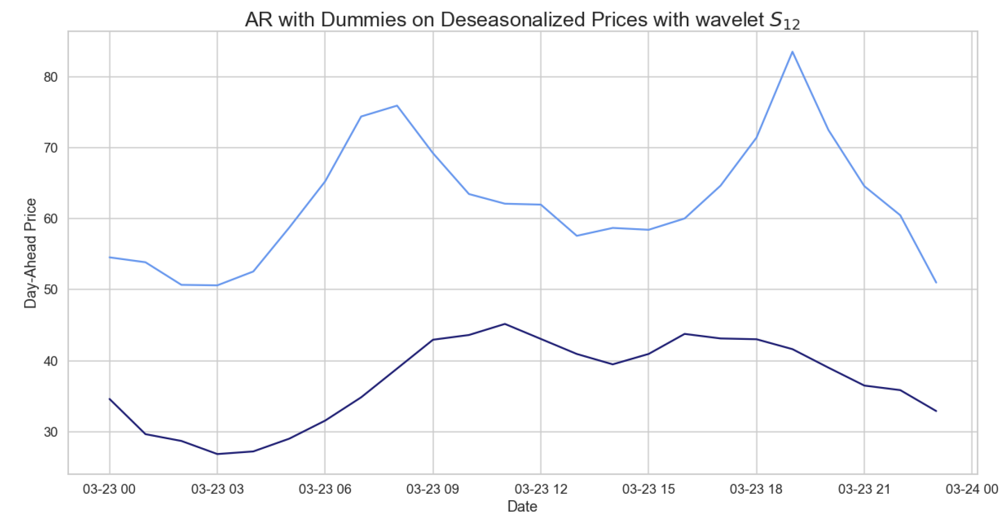
In what follows, we consider the results obtained on deseasonalized daily hourly prices with wavelet $S_{12}$, applying the model explained in Section 2. In

Table 19. RMSE of the AR with the dummies model of different training sets for testing one day on the hourly deseasonalized prices.

AR with Dummies
Training Period	RMSE
2020	26.1521
Spring–Summer	43.4731
Autumn–Winter	39.1706

, we observe the errors of the AR model with dummies. These errors are larger than those obtained with SARIMA and ARIMA, probably because we are not considering the exogenous variables. Figure 13 shows the daily hourly prices and those predicted by the latter model, which are very far from the actual prices. Indeed, they are characterized by two distinct peaks at around 9AM and 7PM, respectively, which are not predicted by the model itself.

5.5. XGBoost

In order to apply the XGBoost model, we have to first select characterizing features, e.g., time, quarter, month, year, day of the week/month/year, and week of the year, of our time series in order to cast the latter into a supervised learning problem. Next, we identify the so-called training set, composed of Xtrain and ytrain. The former is defined on the previously calculated features, while the latter contains the German market electricity prices. Subsequently, we focus on the objective function hyperparameters defined by a training loss and a regularization term. In particular, the training loss indicates how predictive our model is with respect to the training data, according to the MSE measure, while the regularization term controls the model complexity, allowing us to avoid overfitting. For the latter, we consider the $L_1$ regularization with $\alpha =0.1$.

After the model has been fitted on Xtrain and ytrain, the XGBoost library allows us to display the feature importance. In our case, features are ordered (from heavier to lighter ones) as follows: hour, day of the year, day of the week, day of the month, month, and quarter, and we can then forecast prices of the test set based on Xtest.

5.5.1. Daily Average Price

Running the model on daily average prices over two different time windows, we obtain the results shown in

Table 20. RMSE of XGBoost model on different training and test periods for the daily average prices.

XGBoost
Training Period	Test Period	RMSE
2020	2021	90.1138
2020–2021	2022	148.2663

. The XGBoost library provides the feature importance, as shown in Figure 14, which manifests the features that most influence our endogenous variable, i.e., average electricity prices, in the model with a training set over autumn–winter that predicts two weeks.

Table 21. RMSE of the XGBoost model on different training periods for testing two weeks in 2021 on the daily average prices.

XGBoost
Training Period	Test Period	RMSE
2020	two weeks in 2021	46.6614
Spring–Summer	two weeks in 2021	47.8949
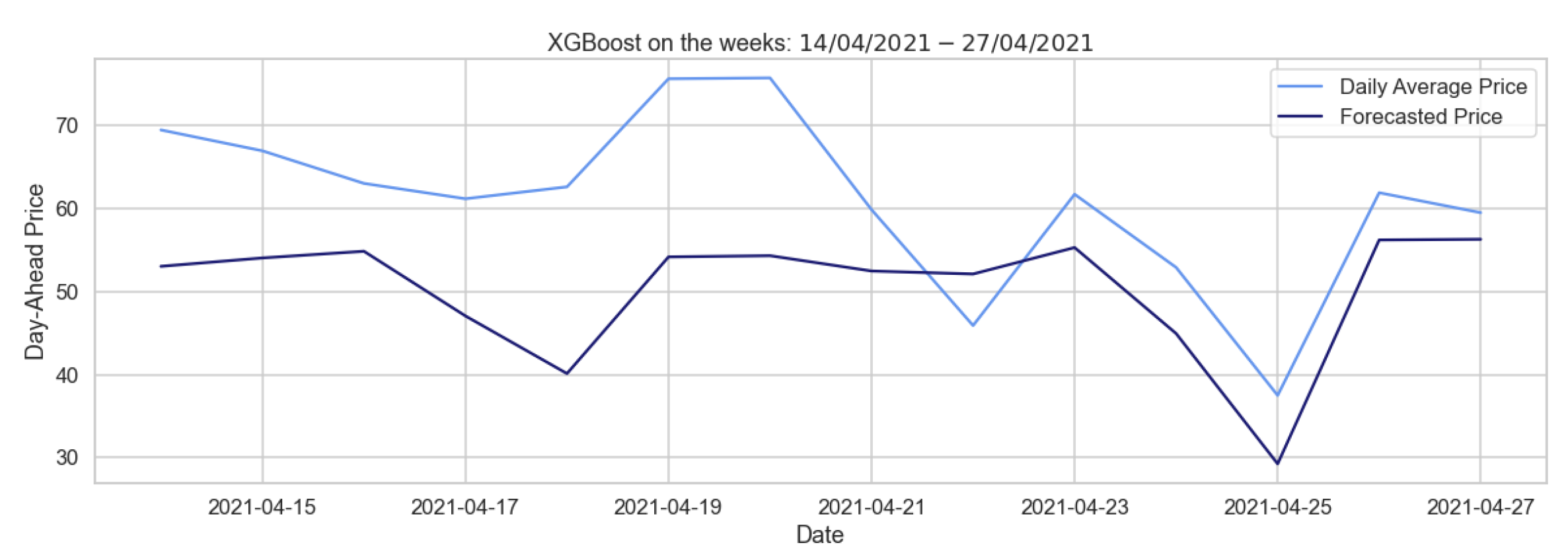
Autumn–Winter	two weeks in 2021	13.2064

shows the errors obtained from the forecasts over different training periods in the two-week forecast, which are not particularly encouraging, as the RMSEs are large. The XGBoost model trained on the autumn–winter period only succeeds in identifying a few negative peaks and fails to predict the behavior of the two weeks as a whole, as Figure 15 reveals.

5.5.2. Hourly Daily Price

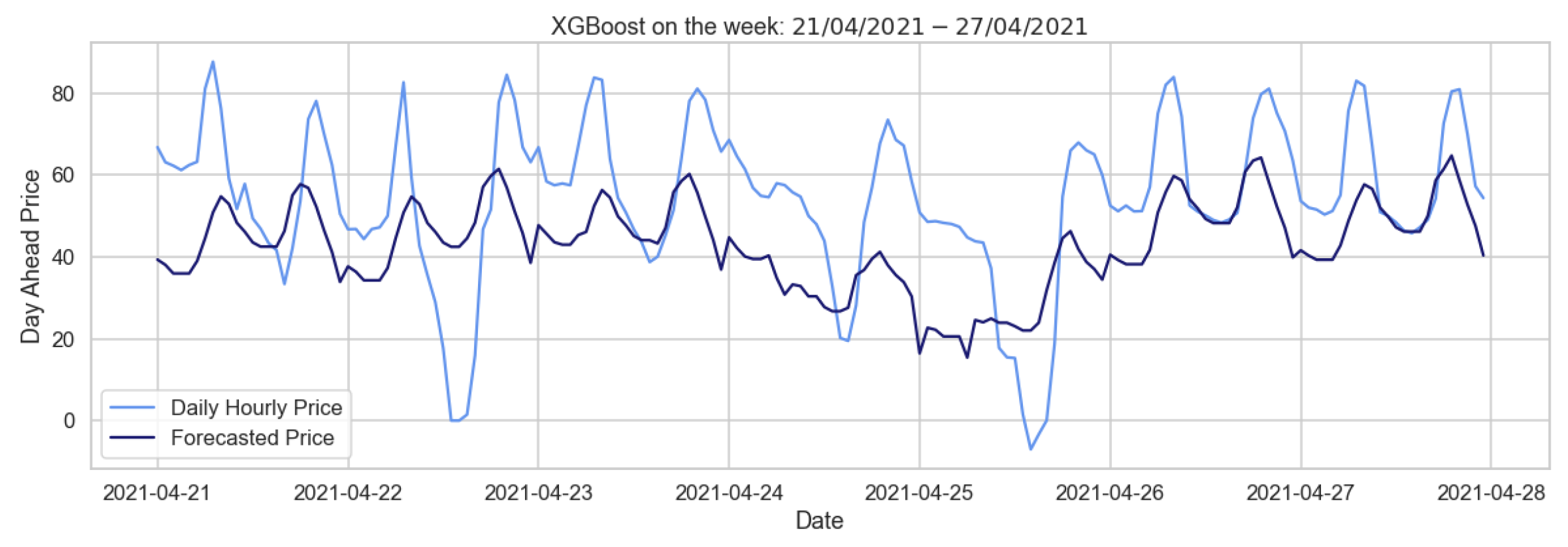
Here we present the XGBoost performed on the daily hourly prices, first in the case of one month forecasts, showing that this model is more accurate than the naive benchmark, and less precise when compared with ARIMA and SARIMA. The results obtained in the weekly and hourly forecasts and displayed in

Table 22. RMSE of the XGBoost model of one month in 2021 for the daily hourly prices.

XGBoost
Training Period	Test Period	RMSE
2020	one month in 2021	122.8169
Spring–Summer	one month in 2021	114.8268
Autumn–Winter	one month in 2021	123.3496

and

Table 23. RMSE of the XGBoost model of different training periods for testing one week in 2021 on the daily hourly prices.

XGBoost
Training Period	Test Period	RMSE
2020	one week in 2021	42.4270
Spring–Summer	one week in 2021	41.3770
Autumn–Winter	one week in 2021	19.7381

clearly appear as large errors, considering the RMSEs, excluding the case where autumn and winter 2020–2021 are used as the training set.

Therfore, as shown in Figure 16, which depicts the forecast for the week of April 2021, this model predicts the regular behavior quite well, while failing to predict the positive and negative price peaks characterizing the German market. In the hourly pricing scenario,

Table 24. RMSE of the XGBoost model of different training periods for testing one day in 2021.

XGBoost
Training Period	Test Period	RMSE
2020	one day in 2021	40.3105
Spring–Summer	one day in 2021	40.9339
Autumn–Winter	one day in 2021	7.7653

illustrates that the XGBoost model works well when utilizing autumn–winter as the training period. Summing up, the XGBoost model performs better than the naive benchmark, even if it shows considerable errors when applied to our data, probably because of their irregularity. A second possible factor is that we are considering variables with similar characteristics as exogenous ones.

5.6. Selection of the Network Structure

Neural networks require input data series to be characterized by low variance levels; otherwise, the associated training process requires exponentially (in volatility level) growing computational time with a low probability of pattern-learning. A possible solution can be found in scaling our time series, hence by a standardization and transformation approach. We consider the median and median absolute deviation (MAD) to avoid the above-mentioned potential delay. In addition, the NN can be used to model univariate time series forecasting problems, but we can not apply them directly to the time series as we did with ARIMA. Rather, we transformed the time series into a multivariate input sample, where each sample has a specific number of time steps, and the output is the value of a single step.

The most common technique for choosing the number of hidden layers and the number of hidden neurons is through experiments since there is not a systematic procedure to find them, unlike for ARIMA; see Section 5.3.2. The neural network must be trained; i.e., examples of the problem to be solved must be presented to the network, then connection weights must be adjusted based on the difference between the output obtained and the desired data (ground truth). On the daily average prices, we implemented a simple RNN, but this did not provide noteworthy results, as by definition it has no memory cell compared to LSTM.

5.6.1. LSTM

Our data need to be normalized, and after that we split the normalized time series into training and test sets; then, we made the time series a multivariate sample as described at the beginning of this section. At this point, we obtained as Xtrain and Xtest, two vectors of dimension $(n,2)$, where n denotes the time windows chosen as input and test, respectively, containing the electricity prices. In our LSTM, we have chosen the Adam algorithm, a stochastic gradient descent method based on an adaptive estimation of first and second order moments (see [26]), as the optimizer with a learning rate of 0.001. In all the Neural Network-based methods, we considered mean square error as the loss function to be minimized throughout the training process, while all the NNs are defined with LSTM hidden layers followed by a dropout one that randomly sets input to zero with a frequency given by the rate specified at each step during the training. Instead, non-zero inputs are scaled up by $1/(1-rate)$, and the batch size defines the number of samples to work on before the internal parameters are updated, usually 32, 64, 128, and 256.

Daily Average Price

We show the results obtained on the LSTM model on the daily average prices using different training and test sets. The model chosen to predict the daily average prices for the year 2021 relies on a NN composed of 4 layers, namely: input, hidden, dropout, and output. In particular, the hidden layer has 300 LSTM cells followed by a dropout layer with rate = 0.4, which acts as a regularizing operator reducing possible overfitting, while a fully connected layer with one neuron is chosen as the output layer. Let us underline that we exploited the Keras library, hence using classes for the layers ‘LSTM’, ‘Dropout’, and ‘Dense’.

In

Table 25. RMSE of the LSTM of training period 2020 for testing one year on the daily average prices.

LSTM with One Hidden Layer
Training Period	Epochs	RMSE
2020	250	34.0001

, we observe the results obtained from the training of an LSTM with a training set of one year and a test set of the following year. Our NN is trained for 250 epochs starting with arbitrary weights, which are updated at each step, minimizing the loss function chosen; in our case, this is the MSE with Adam optimizer, in which the learning rate is 0.001, and the batch size is 60.

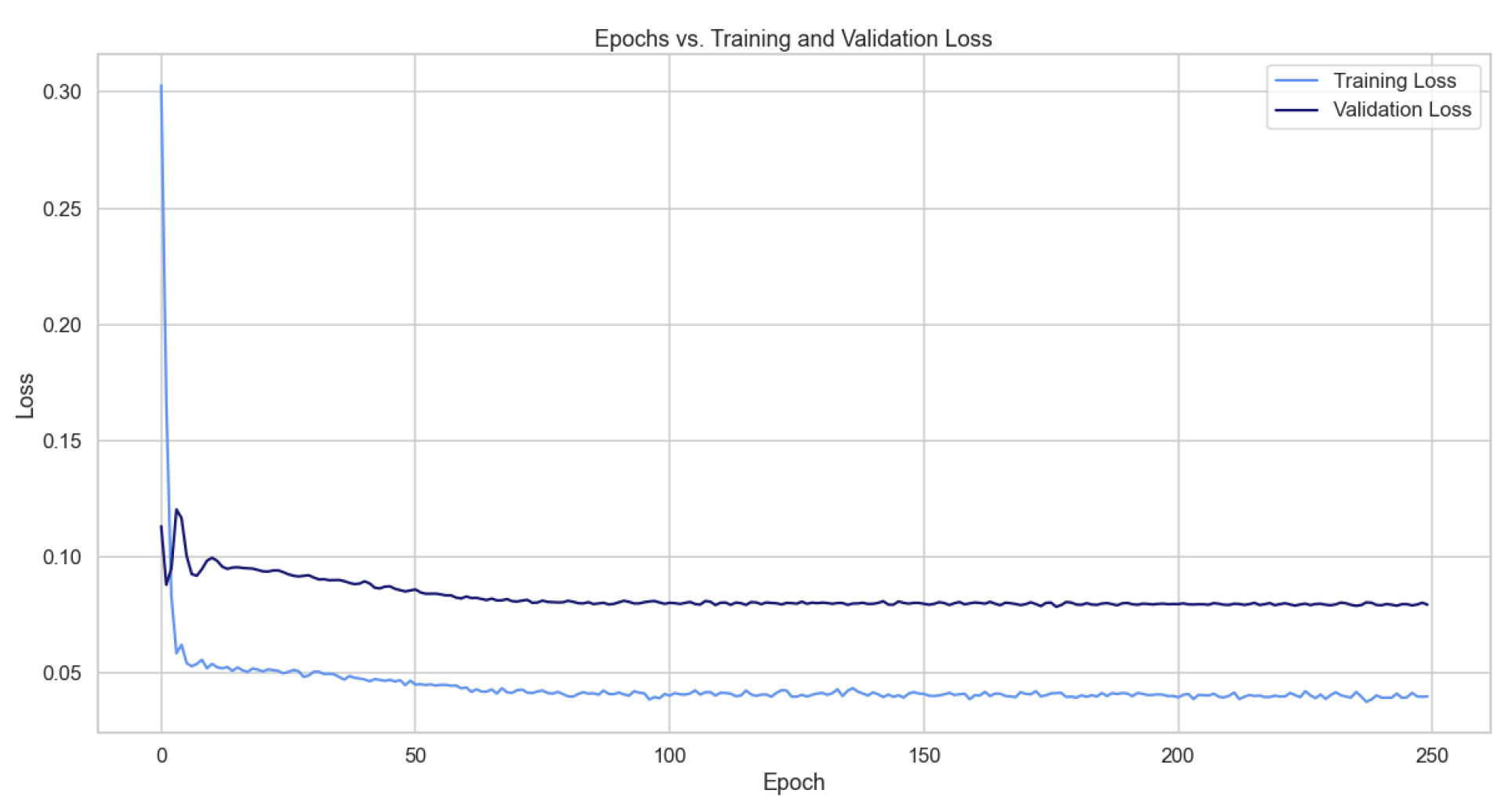
Furthermore, during the training of the NN, we use the month of December 2020 as the validation set; for more details please refer to Appendix A, Figure A1. The result displayed in Table 25 and Figure 17 shows that this NN performs very well on our time series; in fact, the RMSE is lower compared to all the models analyzed before.

The LSTM architecture for predicting mid-2022 is defined with input and output layers as in one of the previous models, while it has 2 hidden layers of 300 LSTM cells each, both followed by a dropout layer with rate 0.2. The training is done with the same optimizer and loss function.

Table 26. RMSE of LSTM of training period 2020–2021 for testing mid-2022 on the daily average prices.

LSTM with Two Hidden Layers
Training Period	Epochs	RMSE
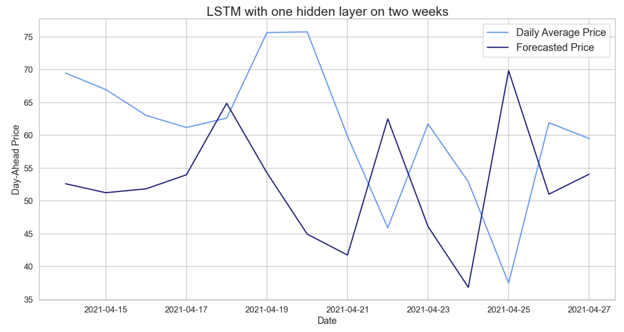
2020–2021	250	57.8398

shows a smaller RMSE, i.e., a better forecast; however, even the LSTM does not perform very well in the case of this forecast. The price behavior in 2022 is totally irregular and different from previous years under consideration. Finally, in order to predict two weeks of daily average prices in 2021, we implemented LSTMs with a single hidden layer defined as an LSTM of 400 cells followed by a dropout layer with rate 0.2.

The results obtained from this LSTM, in

Table 27. RMSE of the LSTM model of different training periods for testing two weeks in 2021 on daily average prices.

LSTM with One Hidden Layer
Training Period	Hidden Layers	Epochs	RMSE
2020	400 units	300	11.0914
Spring–Summer	400 units	300	9.5359
Autumn–Winter	400 units	300	13.8709

, are not optimal; if we compare them to the models previously analyzed on the same training and test sets, they are slightly lower. Figure 18 suggests that our LSTM predicts well the general behavior, excluding the fact that it has a lower price range, which is due to the fact that our model can not predict the trend in our time series.

Hourly Daily Price

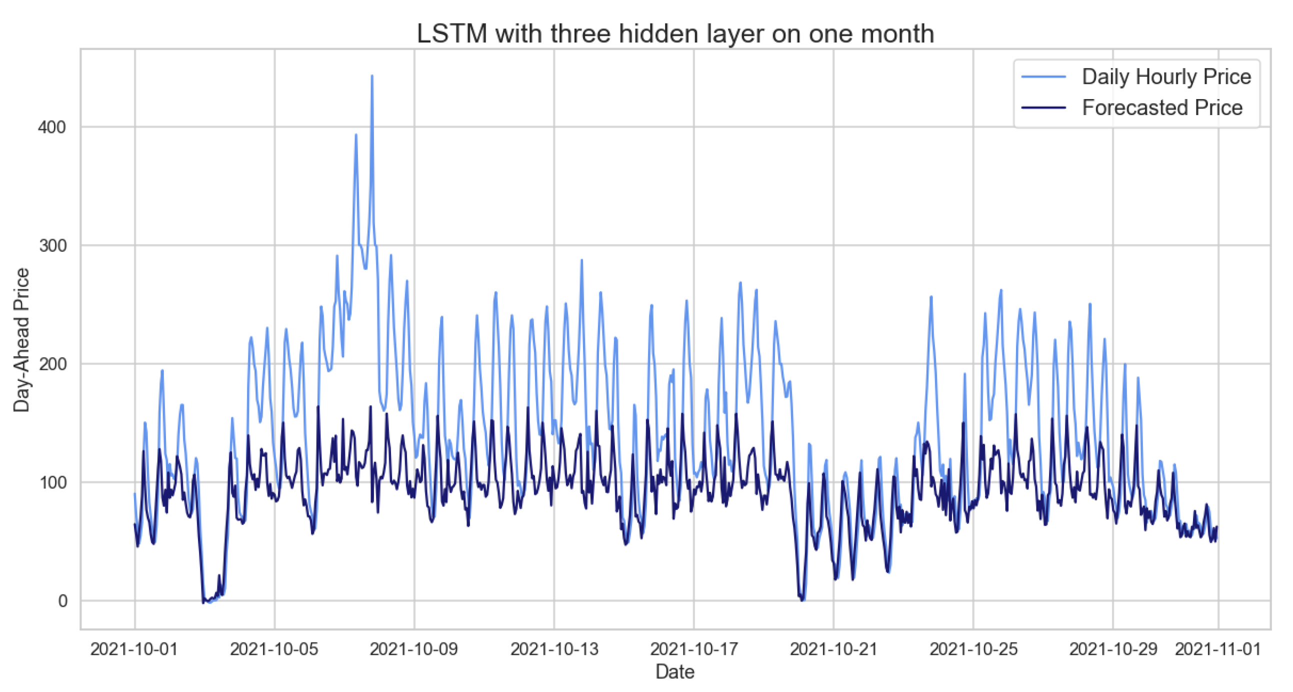
Here we report the results obtained using different training and testing periods on hourly data, enabling us to provide the NN significantly more data than those within the previous subsection, which typically results in improved accuracy. Each of the three hidden layers in the first NN, which has 300 LSTM cells in each, is followed by a dropout layer whose purpose is to prevent overfitting at a rate of 0.2. Moreover, the training is carried out with a batch size of 60.

Both the 2020 training and the autumn–winter training adopt the initial neural network with the previously described architecture. The amount of data available, notably in the case of 2020, and the increased complexity of the neural network itself are undoubtedly responsible for the fact that in both situations the training implementation time takes a few minutes. The neural network, implemented considering spring–summer as the training period, has two LSTM layers with 300 cells each, followed by a dropout layer with a rate of 0.2 and batch size of 60.

Table 28. RMSE of the LSTM model of different training periods for testing one month in 2021.

LSTM with Different Number of Hidden Layers
Training Period	Epochs	LSTM Layers	RMSE
2020	300	3	67.5297
Spring–Summer	300	2	75.1064
Autumn–Winter	300	3	74.7541

presents the RMSE of these NNs, which have been verified as accurate after looking at the loss functions of both the training and validation sets. However, a closer look at Figure 19 suggests that LSTM is better able to represent the behavior of the time series than ARIMA, even though the RMSE of these NNs is marginally greater than the one achieved with the ARIMA model in Table 15.

The predictions generated by the LSTM trained on 2020 accurately forecast negative peaks, which were barely predicted by the other models. One-week forecasts based on 2020 hourly prices are computed via a NN with three hidden LSTM layers, with each having a unit size of 300, followed–as broadly explained–by a 0.2 rate dropout. In the spring–summer training, we define two LSTMs with 250 units each, whereas in the autumn–winter training period, we used two LSTMs with 300 units each. We take into consideration that the first NN’s batch size is 60, while the other NNs’ batches are 30.

The errors from the recently introduced neural networks are shown in

Table 29. RMSE of the LSTM model of different training periods for testing one week in 2021.

LSTM with Different Numbers of Hidden Layers
Training Period	Epochs	RMSE
2020	300	11.3126
Spring–Summer	150	14.3904
Autumn–Winter	250	12.6480

and

Table 30. RMSE of the LSTM model for different training periods for testing one day in 2021.

LSTM with Different Numbers of Hidden Layers
Training Period	Epochs	RMSE
2020	250	7.2073
Spring–Summer	250	8.2753
Autumn–Winter	250	8.2147

, and during this test period, the LSTM remains the most accurate model. In order to estimate the hourly prices of a day on three training time windows, two distinct NNs are designed. With one hidden layer made up of 300 LSTM cells spread throughout 250 epochs, the one trained on 2020 and autumn–winter is the same. The single hidden layer with 500 units was chosen as the NN using spring–summer as the training set.

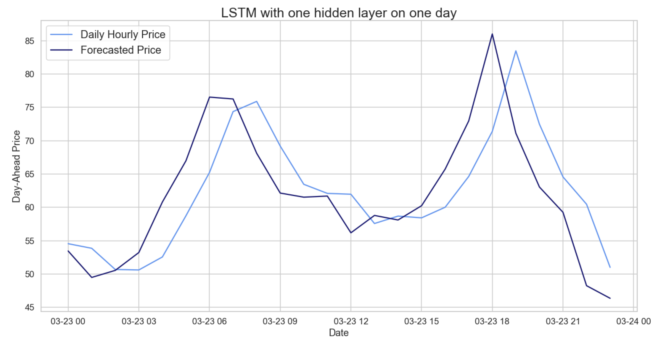
We see that the LSTM is the best model among the tested ones to predict our data. Comparing the hourly prices predicted by the LSTM with the actual prices (Figure 20), we can see how accurately the behavior and peaks are predicted.

6. Conclusions

In the present work, we compared statistical, similar-day, and machine learning approaches to the electricity price forecasting problem with respect to electricity prices of the German market, within the period ranging from 2020 to the middle of 2022. The latter part of the period was characterized by a high degree of volatility, with several ups and downs and irregular seasonality components, caused in part by exogenous socio-political events as the well known COVID-19 pandemic, the climate-related energy crisis, and the Russia–Ukraine war. Our analysis has shown that an LSTM-based approach outperforms all other models when evaluating a medium-term forecast by using daily average prices, as well as when dealing with short-term predictions based on hourly prices.

We have also shown that removing the long trend seasonal component (LTSC) and applying the ARIMA model on deseasonalized prices leads to error mitigation. Unfortunately, this model worked poorly when we examined plots emphasizing differences between the actual and forecast values. The XGBoost model performed better than the naive benchmark model, even if predicted prices are significantly less than the ones obtained with SARIMA and ARIMA.

As a result of our analysis, we claim that exogenous variables such as day-ahead system load forecasts and day-ahead wind power generation may be taken into account to improve obtained forecasts by exploiting more structured models, as, e.g., the neural basis expansion analysis with exogeneous variables (NBEATSx) one, recently introduced as an extension of the neural basis expansion analysis (NBEATS) approach. A possible further improvement could be achieved studying outliers’ behavior; i.e., the predictions of “normal” prices and spiky prices are carried out and then compared. Further possible alternatives within the field of electricity price forecasting research rely on hybrid models, i.e., models obtained by combining statistical and NN models. However, as noted by [3,4], the hybrid models explored so far do not allow the claim that they are superior to the simpler DL-based models. In fact, no suitable study has yet been established to exhibit the best parts of such hybrid models and compare them to the state of the art. In conclusion, this study should be extended by comparing the LSTM model with another non-linear model, such as SARFIMA [27], which allows for series to be fractionally integrated.

Recently, there have been several works focused on stocks [28], cryptocurrencies [29], commodities [30,31], and so on. In a follow-up paper, we will present all the basic ideas of these different methods in the various application areas and briefly explain our proposed approaches to the aforementioned methods, including new work in the field of price forecasting.

References

- Zema, T.; Sulich, A. Models of Electricity Price Forecasting: Bibliometric Research. Energies 2022, 15, 5642. [Google Scholar] [CrossRef]
- Nowotarski, J.; Weron, R. Recent advances in electricity price forecasting: A review of probabilistic forecasting. Renew. Sustain. Energy Rev. 2018, 81, 1548–1568. [Google Scholar] [CrossRef]
- Jędrzejewski, A.; Lago, J.; Marcjasz, G.; Weron, R. Electricity Price Forecasting: The Dawn of Machine Learning. IEEE Power Ener. Mag. 2022, 20, 24–31. [Google Scholar] [CrossRef]
- Lago, J.; Marcjasz, G.; De Schutter, B.; Weron, R. Forecasting day-ahead electricity prices: A review of state-of-the-art algorithms, best practices and an open-access benchmark. Appl. Energy 2021, 293, 116983. [Google Scholar] [CrossRef]
- Lago, J.; De Ridder, F.; De Schutter, B. Forecasting spot electricity prices: Deep learning approaches and empirical comparison of traditional algorithms. Appl. Energy 2018, 221, 386–405. [Google Scholar] [CrossRef]
- Burger, B. Power Generation in Germany-Assessment of 2017; Fraunhofer-Gesellschaft: Munich, Germany, 2018; Volume 18, Available online: https://www.ise.fraunhofer.de/content/dam/ise/en/documents/publications/studies/Stromerzeugung_2017_e.pdf (accessed on 9 March 2023).
- Narajewski, M. Probabilistic forecasting of German electricity imbalance prices. Energies 2022, 15, 4976. [Google Scholar] [CrossRef]
- Nitka, W.; Serafin, T.; Sotiros, D. Forecasting Electricity Prices: Autoregressive Hybrid Nearest Neighbors (ARHNN) Method. In Proceedings of the Computational Science—ICCS 2021, Kolkata, India, 15–18 December 2021; Paszynski, M., Kranzlmüller, D., Krzhizhanovskaya, V.V., Dongarra, J.J., Sloot, P.M., Eds.; Springer: Cham, Switzerland, 2021; pp. 312–325. [Google Scholar]
- Nasiadka, J.; Nitka, W.; Weron, R. Calibration window selection based on change-point detection for forecasting electricity prices. arXiv 2022, arXiv:2204.00872. [Google Scholar]
- Bollerslev, T. Generalized autoregressive conditional heteroskedasticity. J. Econom. 1986, 31, 307–327. [Google Scholar] [CrossRef] [Green Version]
- Novak, J.; Cañas, A. The origins of the concept mapping tool and the continuing evolution of the tool. Inf. Vis. 2006, 5, 175–184. [Google Scholar] [CrossRef]
- Makridakis, S.; Hibon, M. ARMA Models and the Box-Jenkins Methodology. J. Forecast. 1997, 16, 147–163. [Google Scholar] [CrossRef]
- Chen, T.; Guestrin, C. XGBoost: A scalable Tree Boosting System. In Proceedings of the 22nd ACM SIGKDD International Conference on Knowledge Discovery and Data Mining (KDD ’16), San Francisco, CA, USA, 13–17 August 2016; ACM: New York, NY, USA, 2016; pp. 785–794. [Google Scholar]
- XGBoost. 2021. Available online: https://xgboost.readthedocs.io/en/stable/ (accessed on 27 October 2022).
- Saâdaoui, F.; Rabbouch, H. A wavelet-based hybrid neural network for short-term electricity prices forecasting. Artif. Intell. Rev. 2019, 52, 649–669. [Google Scholar] [CrossRef]
- Hochreiter, S.; Schmidhuber, J. Long Short-Term Memory. Neural Comput. 1997, 9, 1735–1780. [Google Scholar] [CrossRef] [PubMed]
- Kuo, P.; Huang, C. An Electricity Price Forecasting Model by Hybrid Structured Deep Neural Networks. Sustainability 2018, 10, 1280. [Google Scholar] [CrossRef] [Green Version]
- Weron, R. Electricity Price forecasting: A review of the state of the art with a look into the future. Int. J. Forecast. 2014, 30, 1030–1081. [Google Scholar] [CrossRef] [Green Version]
- Weron, R. Modeling and Forecasting Electricity Loads and Prices: A Statistical Approach; John Wiley & Sons: Hoboken, NJ, USA, 2007; Volume 403. [Google Scholar]
- Jędrzejewski, A.; Marcjasz, G.; Weron, R. Importance of the long-term seasonal component in day-ahead electricity price forecasting revisited: Parameter-rich models estimated via the LASSO. Energies 2021, 14, 3249. [Google Scholar] [CrossRef]
- Lee, G.; Gommers, L.; Waselewski, F.; Wohlfahrt, K.; O’Leary, A. PyWavelets: A Python package for wavelet analysis. J. Open Source Softw. 2019, 4, 1237. [Google Scholar] [CrossRef]
- Box, G.E.P.; Jenkins, G.M.; Reinsel, G.; Ljung, G. Time Series Analysis: Forecasting and Control; Wiley: San Francisco, CA, USA, 2015. [Google Scholar]
- Tang, Z.; De Almeida, C.; Fishwick, P.A. Time series forecasting using neural networks vs. Box-Jenkins methodology. Simulation 1991, 57, 303–310. [Google Scholar] [CrossRef]
- Choon, O.H.; Chuin, J.L.T. A Comparison of Neural Network Methods and Box-Jenkins Model in Time Series Analysis. In Proceedings of the Fourth IASTED International Conference on Advances in Computer Science and Technology, Langkawi, Malaysia, 2–4 April 2008; ACTA Press: Anaheim, CA, USA, 2008; pp. 344–350. [Google Scholar]
- De-Graft Acqua, H. Comparison of Akaike information criterion (AIC) and Bayesian information criterion (BIC) in selection of an asymmetric price relationship. J. Devel. Agric. Econ. 2010, 2, 1–6. [Google Scholar]
- Diederik, P.K.; Ba, J. Adam: A Method for Stochastic Optimization. arXiv 2014, arXiv:1412.6980. [Google Scholar]
- Porter-Hudak, S. An Application of the Seasonal Fractionally Differenced Model to the Monetary Aggregates. J. Am. Stat. Assoc. 1990, 85, 338–344. [Google Scholar] [CrossRef]
- Lu, W.; Li, J.; Wang, J.; Qin, L. A CNN-BiLSTM-AM method for stock price prediction. Neural Comput. Appl. 2021, 33, 4741–4753. [Google Scholar] [CrossRef]
- Guarino, A.; Grilli, L.; Santoro, D.; Messina, F.; Zaccagnino, R. To learn or not to learn? Evaluating autonomous, adaptive, automated traders in cryptocurrencies financial bubbles. Neural Comput. Appl. 2022, 34, 20715–20756. [Google Scholar] [CrossRef]
- Yuan, C.Z.; Ling, S.K. Long short-term memory model based agriculture commodity price prediction application. In Proceedings of the 2020 2nd International Conference on Information Technology and Computer Communications, Kuala Lumpur, Malaysia, 12–14 August 2020; pp. 43–49. [Google Scholar]
- Gu, Y.H.; Jin, D.; Yin, H.; Zheng, R.; Piao, X.; Yoo, S.J. Forecasting agricultural commodity prices using dual input attention LSTM. Agriculture 2022, 12, 256. [Google Scholar] [CrossRef]
Figure 1.
Block of long short term memory at any timestamp t.
Figure 2.
Comparison of target and forecast values for one day with the naive benchmark model for daily hourly prices on 23 March for the years 2020 and 2021.
Figure 3.
Comparison of target and forecast values for mid-2022 using 2020–2021 as the training set with for daily average prices.
Figure 4.
Comparison of target and forecast values for two weeks in 2021 using autumn–winter 2020–2021 as the training set with on daily average prices.
Figure 5.
Comparison of target and forecast values for one week in 2021 using autumn–winter as the training set with .
Figure 6.
Comparison of target and forecast values for one day in 2021 using 2020 as the training set with .
Figure 7.
Figure of the long trend seasonal component (LTSC) based on wavelets , , and for the daily average prices.
Figure 8.
Figure showing the deseasonalized prices based on wavelet for the daily average prices.
Figure 9.
Figure showing the deseasonalized prices based on wavelet for the daily hourly prices.
Figure 10.
Comparison of target and forecast values for 2021 using 2020 as training set with for daily average prices.
Figure 11.
Comparison of target and forecast values for two weeks in 2021 using spring–summer as the training set with ARIMA for the deseasonalized daily average prices.
Figure 12.
Comparison of target and forecast values for one week using 2020 as the training set with for daily hourly prices.
Figure 13.
Comparison of target and forecast values with AR dummies for one day in 2021 using 2020 as training set on daily hourly prices.
Figure 14.
Feature importance of the XGBoost on daily average prices for two weeks using the autumn–winter period as the training set.
Figure 15.
Comparison of target and forecast with XGBoost on daily average prices for two weeks using autumn–winter as the training set.
Figure 16.
Comparison of target and forecast values for one week using autumn–winter as the training set with the XGBoost model on daily hourly prices.
Figure 17.
Comparison of target and forecast values for the year 2021 using 2020 as the training set with the LSTM model on daily average prices.
Figure 18.
Comparison of target and forecast values for two weeks using 2020 as the training set with the LSTM model on daily average prices.
Figure 19.
Comparison of target and forecast values for one month using 2020 as the training set with the LSTM model on daily hourly prices.
Figure 20.
Comparison of target and forecast values for one day using 2020 as the training set with the LSTM model on daily hourly prices.