An Interval-Valued Three-Way Decision Model Based on Cumulative Prospect Theory

Abstract

In interval-valued three-way decision, the reflection of decision-makers’ preference under the full consideration of interval-valued characteristics is particularly important. In this paper, we propose an interval-valued three-way decision model based on the cumulative prospect theory. First, by means of the interval distance measurement method, the loss function and the gain function are constructed to reflect the differences of interval radius and expectation simultaneously. Second, combined with the reference point, the prospect value function is utilized to reflect decision-makers’ different risk preferences for gains and losses. Third, the calculation method of cumulative prospect value for taking action is given through the transformation of the prospect value function and cumulative weight function. Then, the new decision rules are deduced based on the principle of maximizing the cumulative prospect value. Finally, in order to verify the effectiveness and feasibility of the algorithm, the prospect value for decision-making and threshold changes are analyzed under different risk attitudes and different radii of the interval-valued decision model. In addition, compared with the interval-valued decision rough set model, our method in this paper has better decision prospects.

1. Introduction

The three-way decision theory (TWD), proposed by Yao [1] in 2009, was applied to address uncertain information based on the rough set theory. As an extension of two-way decisions in acceptance or rejection, it took the boundary region as the third decision rule on the basis of the positive region and the negative region, that is, to make decision of non-commitment. In real life, people are often faced with a significant amount of decision-making problems, and how to effectively evaluate decision risk for reducing decision loss becomes an important research question. When information is insufficient or inadequate, huge losses are produced if we reject a good decision or accept a bad one. Therefore, increasing the non-commitment decision rules is can minimize the losses of decisions in the three-way decision theory. In recent years, the three-way decision theory has gradually become an important decision-making method, which has been widely applied in the fields of information management, medical treatment, risk insurance investment, etc. [2,3,4,5].

In the decision-theoretic rough sets (DTRSs), with the aid of the loss function, the expected loss under three different decision rules was calculated according to Bayesian decision procedure, and then the threshold was obtained from the principle of minimum expected loss [6]. Xu et al. [7] analyzed the characteristics of the loss function in DTRSs and the logical relationship between the loss function and threshold, and then proposed a threshold calculation method based on the logical relationship between decision loss objective functions. Considering that the difference in equivalence classes will affect the decision result, Xie et al. [8] proposed an adaptive threshold calculation method based on similarity measure. Certain prior knowledge was used to presuppose the loss function, which led to some limitations in the application of the three-way decision theory. Without the loss function, Chen et al. [9] proposed an optimal threshold algorithm based on grid search, aiming at minimizing the sum of decision losses. Jia et al. [10] proposed a simulated annealing algorithm to address the optimal threshold problem, and verified the advantage of the algorithm in running time. Two thresholds, $\alpha$ and $\beta$, which are calculated according to the principle of minimum risk loss in decision-making, cannot reflect the subjective initiative of decision-makers well. Zhang et al. [11] introduced the utility theory, by replacing the loss function with the utility function and proposing a utility three-way decision model (UTWD) in order to reflect the decision-maker’s attitude toward risk better.

The prospect theory (PT), established by Kahneman and Tversky in 1979 [12], reveals the reason and essence of people’s decision-making behavior deviating from rationality under uncertainty. It can better reflect the decision-making preferences of decision-makers, supplement the deficiency of the expected utility theory, and has been widely applied in multi-attribute decision-making [13,14,15,16]. The cumulative prospect theory (CPT) was proposed in 1992 [17], considering that the PT cannot solve the stochastic dominance problem, and it has a wider application range compared with the PT [18,19]. Wang et al. [20] thought that the utility theory, which relies on intuitive decision-making, can reduce the complexity of decision-making, but cannot reflect the attitude toward the loss when facing risks. Therefore, they introduced the PT into a three-way decision model and proposed the prospect theory-based three-way decision model (PTWD). On the basis of the PTWD, Wang et al. [21] introduced the CPT to linearize the weight function further and proposed a three-way decision model based on the cumulative prospect theory (CPTWD).

The data involved in prospect theory are all in the form of single value, while the complexity of the environment and the existence of irrational factors, such as decision-makers’ subjective preference, emotional thinking, etc., lead to the uncertainty of decision-making risk. Therefore, it is closer to real life by describing the outcome function in prospect theory with interval numbers characterized by multi-value. Yin et al. [22] transformed the interval number into the form of the score function, and introduced the prospect value function to describe the subjective feeling of decision-making. Hu et al. [23], firstly, dispersed the interval number into different finite data, and described the distribution law of the values in the interval value by using the normal distribution function, then obtained the total decision prospect through the weighted average method. Xiong et al. [24] reserved the features of interval value to directly calculate the interval-valued prospect, and then derived the synthetic foreground value of each decision-making rule based on the determination factor rule library. Fan et al. [25] treated the reference point as single value according to the positional relationship between the reference point and the attribute value, and calculated the loss value and the gain value on the basis of the prospect value function. This method only considered the upper bound or the lower bound of the interval in the treatment of the reference point. In addition, when the reference point is included in the attribute value, the loss value and the gain value are both regarded as 0, but in fact, the attribute values including the reference point are also different. Besides interval numbers, Wang et al. [26] used Z-numbers to describe uncertainty in decision-making, and proposed a three-way decision model combined with Z-numbers and the third-generation prospect theory.

Inspired by the above observation, we use interval values to describe the cumulative prospect theory. In order to address interval values, we adopt the interval-valued distance measurement method [27] characterized by similarity to describe the loss value and the gain value. The advantages of the proposed model are summarized as follows.

(1).

Interpret the distance between the two interval values as the benefit of taking action. Since the decision-makers have different attitudes toward loss and gain, the distance between two interval values is studied from two angles, namely the gain distance and the loss distance. It can measure the prospect value more accurately when generated by taking action.

(2).

Combining the value function and interval-valued distance with similar characteristics can better distinguish the difference between different interval values, especially when the two interval values have the same expectation.

(3).

On the basis of [21], using interval values to describe the outcome matrix is more in line with the actual situation. At the same time, the model proposed in this paper can also address the outcome matrix in the form of single values. Thus, it has a wider range of application.

The remainder of this paper is detailed below. In Section 2, some basic concepts of interval value, classical three-way decision model, and cumulative prospect theory are presented. In Section 3, a new method of measuring the prospect value based on the interval value is proposed, and then an interval-valued three-way decision model based on the cumulative prospect theory is constructed. The thresholds and simplified decision rules are further analyzed in Section 4. In Section 5, an example is given to illustrate the effectiveness of our model in distinguishing different interval values; then, the proposed model is compared with the interval number three-way decision model. The whole methods and experiments’ results conclude in Section 6.

2. Preliminaries

2.1. Basic Theory of Intervals

Definition 1

([28]). Let R denote the set of real numbers. For $\forall a^{+}$, $a^{-}\in R$ and $a^{-}\le a^{+}$, then $\tilde{a}=[a^{-},a^{+}]$ is called an interval value, where $a^{-}$ and $a^{+}$ represent the lower and upper bounds of the interval value, respectively. In particular, if $a^{-}=a^{+}$, the interval value degenerates to a real number. Supposing $\tilde{b}=[b^{-},b^{+}]$ is another interval value, if $a^{-}=b^{-}$ and $a^{+}=b^{+}$, we have $\tilde{a}=\tilde{b}$.

Definition 2

([29]). Let $\tilde{a}=[a^{-},a^{+}]$ is an interval value, then $\frac{a^{-}+a^{+}}{2}$ is called the expectation of the interval value $\tilde{a}$, denoted by $m\left(\tilde{a}\right)$. Furthermore, $\frac{a^{+}-a^{-}}{2}$ is called the radius of the interval value $\tilde{a}$, denoted by $r\left(\tilde{a}\right)$.

Evidently, $\tilde{a}=[m\left(\tilde{a}\right)-r\left(\tilde{a}\right),m\left(\tilde{a}\right)+r\left(\tilde{a}\right)]$, that is, the expected value and the radius of the interval can exactly describe an interval value.

Definition 3

([28]). Given two interval values $\tilde{a}=[a^{-},a^{+}]$, $\tilde{b}=[b^{-},b^{+}]$, and a real number k, then define the operational relationship between them as follows:

(1). 

$\tilde{a}+\tilde{b}=[a^{-}+b^{-},a^{+}+b^{+}]$;

(2). 

$\tilde{a}-\tilde{b}=[a^{-}-b^{+},a^{+}-b^{-}]$;

(3). 

$\tilde{a}\tilde{b}=[min(a^{-}{b}^{-},a^{-}{b}^{+},a^{+}{b}^{-},a^{+}{b}^{+}),max(a^{-}{b}^{-},a^{-}{b}^{+},a^{+}{b}^{-},a^{+}{b}^{+})]$;

(4). 

$\tilde{a}/\tilde{b}=[a^{-},a^{+}]\times [1/b^{+},1/b^{-}]$, where $0\notin [b^{-},b^{+}]$;

(5). 

$k\tilde{a}=[k{a}^{-},k{a}^{+}]$, where $k\in R$ and $k\ge 0$.

2.2. Classical Three-Way Decision Model

Let $\Omega =\{X,\neg X\}$ be a set of states, X and $\neg X$ denote that the object belongs to and does not belong to X, respectively. Furthermore, $\mathcal{A}=\{a_P,a_B,a_N\}$ is a set of actions, where $a_P$, $a_B$ and $a_N$ denote three actions of accepting decision, delaying decision, and rejecting decision, respectively. The data from the risk or cost generated by the three actions under the two states are a matrix, as shown in

Table 1. The loss function matrix.

	X	$\neg \mathit{X}$
$a_P$	${\lambda }_{PP}$	${\lambda }_{PN}$
$a_B$	${\lambda }_{BP}$	${\lambda }_{BN}$
$a_N$	${\lambda }_{NP}$	${\lambda }_{NN}$

. When the object belongs to X, ${\lambda }_{PP}$, ${\lambda }_{BP}$ and ${\lambda }_{NP}$ represent the losses of $a_P$, $a_B$, and $a_N$, respectively. Similarly, when the object does not belong to X, ${\lambda }_{PN}$, ${\lambda }_{BN}$, and ${\lambda }_{NN}$ represent the losses incurred for taking actions of $a_P$, $a_B$, and $a_N$, respectively. $Pr\left(X\right|\left[o\right])$ represents the conditional probability of the equivalence class $\left[o\right]$ belonging to X.

Therefore, the expected losses for each of the three actions are calculated as follows:

$\mathcal{R}\left(a_P\right|\left[o\right])={\lambda }_{PP}Pr\left(X\right|\left[o\right])+{\lambda }_{PN}Pr(\neg X|\left[o\right])$,

$\mathcal{R}\left(a_B\right|\left[o\right])={\lambda }_{BP}Pr\left(X\right|\left[o\right])+{\lambda }_{BN}Pr(\neg X|\left[o\right])$,

$\mathcal{R}\left(a_N\right|\left[o\right])={\lambda }_{NP}Pr\left(X\right|\left[o\right])+{\lambda }_{NN}Pr(\neg X|\left[o\right])$.

According to the minimum expected loss rule, three decision rules are obtained as follows [30]:  

$\left(P0\right)$  If $\mathcal{R}\left(a_P\right|\left[o\right])\le \mathcal{R}\left(a_B\right|\left[o\right])$ and $\mathcal{R}\left(a_P\right|\left[o\right])\le \mathcal{R}\left(a_N\right|\left[o\right])$, decide $o\in \mathrm{POS}\left(X\right)$,  

$\left(B0\right)$  If $\mathcal{R}\left(a_B\right|\left[o\right])\le \mathcal{R}\left(a_P\right|\left[o\right])$ and $\mathcal{R}\left(a_B\right|\left[o\right])\le \mathcal{R}\left(a_N\right|\left[o\right])$, decide $o\in \mathrm{BND}\left(X\right)$,  

$\left(N0\right)$  If $\mathcal{R}\left(a_N\right|\left[o\right])\le \mathcal{R}\left(a_P\right|\left[o\right])$ and $\mathcal{R}\left(a_N\right|\left[o\right])\le \mathcal{R}\left(a_B\right|\left[o\right])$, decide $o\in \mathrm{NEG}\left(X\right)$.  

If $({\lambda }_{PN}-{\lambda }_{BN})({\lambda }_{NP}-{\lambda }_{BP})>({\lambda }_{BP}-{\lambda }_{PP})({\lambda }_{BN}-{\lambda }_{NN})$, then the rule $\left(P0\right)-\left(N0\right)$ should be rewritten as follows:  

$\left(P1\right)$  If $Pr\left(X\right|\left[o\right])\ge {\alpha }_1$, decide $o\in \mathrm{POS}\left(X\right)$,  

$\left(B1\right)$  If ${\beta }_1<Pr\left(X\right|\left[o\right])<{\alpha }_1$, decide $o\in \mathrm{BND}\left(X\right)$,  

$\left(N1\right)$  If $Pr\left(X\right|\left[o\right])\le {\beta }_1$, decide $o\in \mathrm{NEG}\left(X\right)$.  

Otherwise, the rule $\left(P0\right)-\left(N0\right)$ should be rewritten as follows:  

$\left(P1\right)$   If $Pr\left(X\right|\left[o\right])\ge {\gamma }_1$, decide $o\in \mathrm{POS}\left(X\right)$,  

$\left(N1\right)$   If $Pr\left(X\right|\left[o\right])<{\gamma }_1$, decide $o\in \mathrm{NEG}\left(X\right)$.

Where, ${\alpha }_1=\frac{({\lambda }_{PN}-{\lambda }_{BN})}{({\lambda }_{PN}-{\lambda }_{BN})+({\lambda }_{BP}-{\lambda }_{PP})}$, ${\beta }_1=\frac{({\lambda }_{BN}-{\lambda }_{NN})}{({\lambda }_{BN}-{\lambda }_{NN})+({\lambda }_{NP}-{\lambda }_{PP})}$, ${\gamma }_1=\frac{({\lambda }_{PN}-{\lambda }_{NN})}{({\lambda }_{PN}-{\lambda }_{NN})+({\lambda }_{NP}-{\lambda }_{PP})}$.

2.3. Cumulative Prospect Theory

Based on bounded rationality, the cumulative prospect theory reflects the risk preference of decision-makers through three parts: the reference point, the value function, and the weight function.

Definition 4

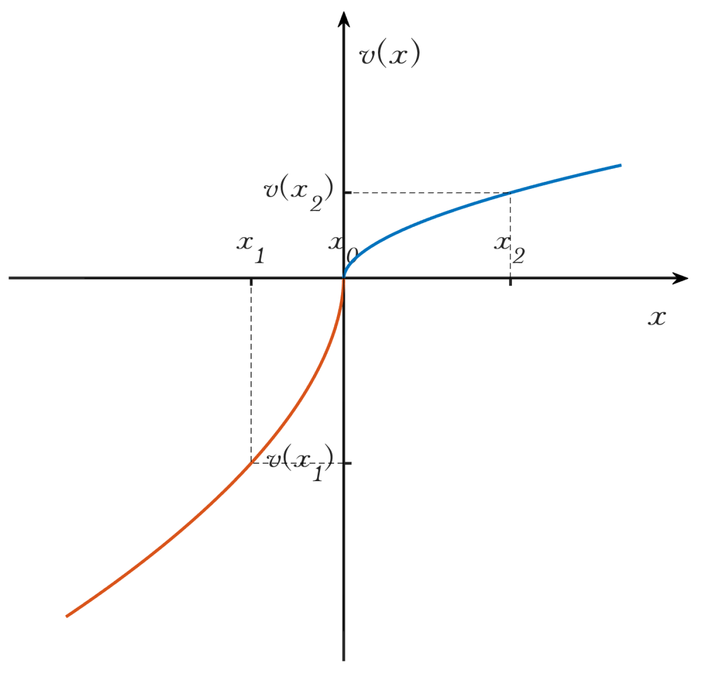
([12]). The value function is to convert the outcome presented by the surface value into the outcome that people have in mind when making decisions, and its specific form is as follows:

$$\nu \left(x\right)=\left\{\begin{array}{cc}{(x-x_0)}^{\mu },\hfill & \hfill x\ge x_0,\\ -\theta {(x_0-x)}^{\upsilon },\hfill & \hfill x<x_0,\end{array}\right.$$

(1)

where x is the outcome and $x_0$ is the reference point selected by decision-makers.

If $x\ge x_0$, the outcome is seen as a gain; otherwise, if $x<x_0$, the outcome is viewed as a loss. $\mu$ and $\upsilon$ ($0<\mu ,\upsilon <1$) are risk attitude coefficients, the larger $\mu$ and $\upsilon$ are, the more inclined decision-makers are to take risks. $\theta$ is the risk aversion coefficient, the larger $\theta$ is, the more sensitive the decision-maker is to loss. Thus, the outcomes can be transformed into decision prospect values, which is shown in Figure 1.

Definition 5

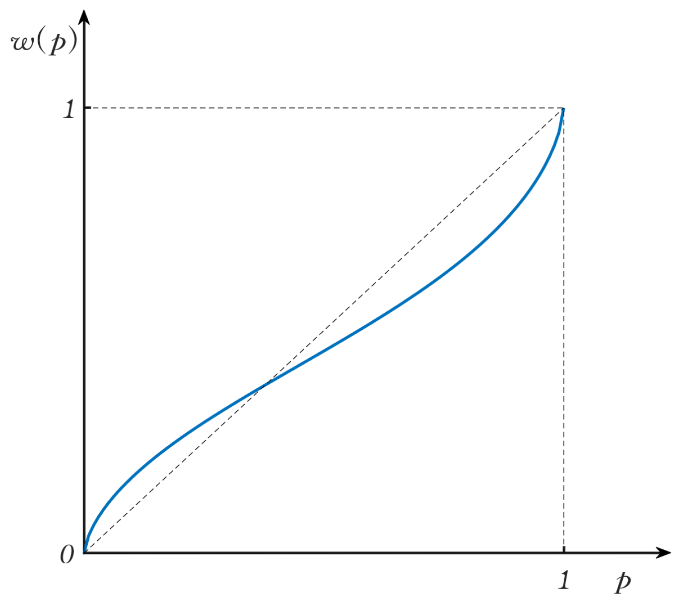
([12]). The weight function is to convert the probability of an event to a decision weight, and its specific form is as follows:

$$\begin{array}{c}\hfill {\varpi }^{+}=\frac{p_h^{\sigma }}{{(p_h^{\sigma }+{(1-p_h)}^{\sigma })}^{\frac{1}{\sigma }}},\\ \hfill {\varpi }^{-}=\frac{p_h^{\delta }}{{(p_h^{\delta }+{(1-p_h)}^{\delta })}^{\frac{1}{\delta }}},\end{array}$$

(2)

where $p_h$ is the conditional probability of an event occurring.

The weight function points out that the decision-maker’s subjective judgment is often inconsistent with the probability axiom when people take some action according to the probability of an event occurring. The weight function presents an inverted “S” curve, as shown in Figure 2, which reflects that decision-makers tend to overestimate the probability of occurrence in small probability events and underestimate the probability of occurrence in large probability events when taking actions.

In the cumulative prospect theory, the result of sorting the benefits generated by each event in ascending order is $x_{-m}<\cdots <x_0<\cdots <x_n$, and the probability of occurrence of the corresponding event is $p=(p_{-m},\cdots ,p_n)$. The corresponding cumulative weight function is expressed as follows [17]:

$${\omega }_h=\left\{\begin{array}{cc}{\varpi }^{+}(p_h+\cdots +p_n)-{\varpi }^{+}(p_{h+1}+\cdots +p_n),\hfill & \hfill h>0,\\ {\varpi }^{-}(p_{-m}+\cdots +p_h)-{\varpi }^{-}(p_{-m}+\cdots +p_{h-1}),\hfill & \hfill h<0,\end{array}\right.$$

(3)

where, $-m\le h\le n$.

Therefore, by conversion of the value function and the weight function, the cumulative prospect value is calculated as follows:

$$\mathcal{V}=\sum _{h=-m}^n{\omega }_h\nu \left(x_h\right).$$

(4)

3. Three-Way Decisions Based on Cumulative Prospect Theory with Interval Value

3.1. Calculation Method of the Value Function

Definition 6

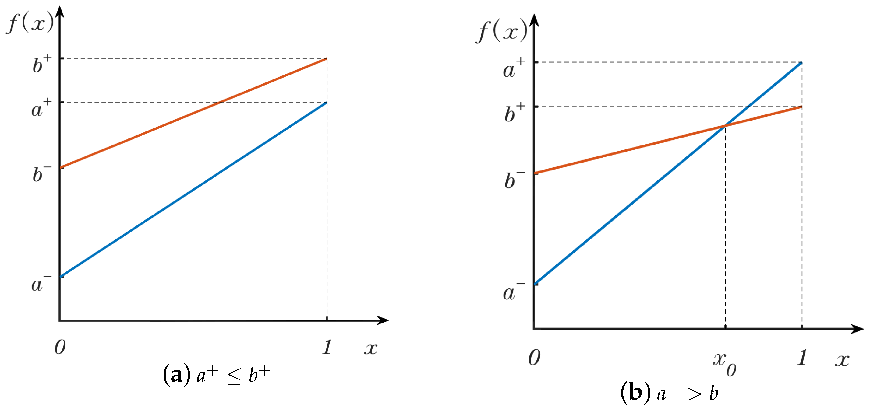
([31]). Given an interval value $\tilde{a}=[a^{-},a^{+}]$. $f_{\tilde{a}}\left(x\right)=a^{-}+(a^{+}-a^{-})x$ is used to determine the position of a number in an interval value $\tilde{a}$, called the location function, where $x\in [0,1]$. $f_{\tilde{a}}\left(1\right)$ and $f_{\tilde{a}}\left(0\right)$ denote the upper and lower bounds of the interval value, respectively. If $a^{-}=a^{+}$, $\tilde{a}$ is a real number, i.e., the location function is a constant function. In addition, another equivalent form of the location function is $f_{\tilde{a}}\left(x\right)=a^{-}+2r\left(\tilde{a}\right)x$.

Let $\tilde{a}=[a^{-},a^{+}]$ and $\tilde{b}=[b^{-},b^{+}]$ be two interval values whose location functions are $f_{\tilde{a}}$ and $f_{\tilde{b}}$, respectively, where $a^{-}\le b^{-}$. As shown in Figure 3a, if $a^{+}\le b^{+}$, the inequality $f_{\tilde{a}}\left(x\right)\le f_{\tilde{b}}\left(x\right)$ always holds on [0, 1]. On the contrary, as shown in Figure 3b, if $a^{+}>b^{+}$, the inequality $f_{\tilde{a}}\left(x\right)\le f_{\tilde{b}}\left(x\right)$ is true when $x\in [0,x_0]$. Furthermore, the inequality $f_{\tilde{a}}\left(x\right)>f_{\tilde{b}}\left(x\right)$ is true when $x\in (x_0,1]$.

Definition 7.

Let an interval value $\tilde{a}=[a^{-},a^{+}]$ denote the outcome interval of taking a certain action, ${\tilde{e}}_k=[e_k^{-},e_k^{+}]$ is the reference point of the kth decision-maker. This means that taking the action is in a state of gain when $f_{\tilde{a}}\left(x\right)\ge f_{{\tilde{e}}_k}\left(x\right)$. On the other hand, when $f_{\tilde{a}}\left(x\right)<f_{{\tilde{e}}_k}\left(x\right)$, it is in a state of loss. Assuming that $\forall a\in \tilde{a}$ and $\forall e_k\in {\tilde{e}}_k$ are uniformly distributed, the loss (L) and gain function (G) are defined as follows with reference to the interval-valued distance measurement method in [27]:

$$L(\tilde{a},{\tilde{e}}_k)={\left({\int }_{{\Omega }_L}{(f_{\tilde{a}}\left(x\right)-f_{{\tilde{e}}_k}\left(x\right))}^{2}dx\right)}^{\frac{1}{2}},$$

(5)

$$G(\tilde{a},{\tilde{e}}_k)={\left({\int }_{{\Omega }_G}{(f_{\tilde{a}}\left(x\right)-f_{{\tilde{e}}_k}\left(x\right))}^{2}dx\right)}^{\frac{1}{2}},$$

(6)

where ${\Omega }_L=\{x\in [0,1]|f_{\tilde{a}}\left(x\right)<f_{{\tilde{e}}_k}\left(x\right)\}$, ${\Omega }_G=\{x\in [0,1]|f_{\tilde{a}}\left(x\right)\ge f_{{\tilde{e}}_k}\left(x\right)\}$.

Example 1.

Let $\tilde{a}=[2,4]$, ${\tilde{e}}_k=[0,7]$. By Definition 6, we have $f_{\tilde{a}}\left(x\right)=a^{-}+(a^{+}-a^{-})x=1+(4-1)x=1+3x$, $f_{\widetilde{e_k}}\left(x\right)=e_k^{-}+(e_k^{+}-e_k^{-})x=0+(7-0)x=7x$, so $f_{\tilde{a}}\left(x\right)-f_{\widetilde{e_k}}\left(x\right)=1-4x$. Then, we get ${\Omega }_L=\{x\in [0,1]|f_{\tilde{a}}\left(x\right)<f_{{\tilde{e}}_k}\left(x\right)\}=\{x\in [0,1]|1+3x<7x\}=(0.25,1]$, ${\Omega }_G=\{x\in [0,1]|f_{\tilde{a}}\left(x\right)\ge f_{{\tilde{e}}_k}\left(x\right)\}=\{x\in [0,1]|1+3x\ge 7x\}=[0,0.25]$. Based on Formula (5), we can calculate that $L(\tilde{a},{\tilde{e}}_k)={\left({\int }_{{\Omega }_L}{(f_{\tilde{a}}\left(x\right)-f_{{\tilde{e}}_k}\left(x\right))}^{2}dx\right)}^{\frac{1}{2}}={\left({\int }_{(0.25,1]}{(1-4x)}^{2}dx\right)}^{\frac{1}{2}}=1.5000$. Similarly, we can also calculate that $G(\tilde{a},{\tilde{e}}_k)={\left({\int }_{{\Omega }_G}{(f_{\tilde{a}}\left(x\right)-f_{{\tilde{e}}_k}\left(x\right))}^{2}dx\right)}^{\frac{1}{2}}={\left({\int }_{[0,0.25]}{(1-4x)}^{2}dx\right)}^{\frac{1}{2}}\approx 0.2887$ based on Formula (6).

According to the coverage of the value between the outcome interval and the reference point, the calculation methods of the loss function and gain function can be divided into the following seven situations:

case1.

If $e_k^{-}=a^{-}$ and $e_k^{+}=a^{+}$, $L(\tilde{a},{\tilde{e}}_k)=0$, $G(\tilde{a},{\tilde{e}}_k)=0$.

case2.

If $e_k^{+}<a^{-}$, we have ${\Omega }_L=\varnothing$ (because of $f_{{\tilde{e}}_k}\left(x\right)\le e_k^{+}<a^{-}\le f_{\tilde{a}}\left(x\right)$), ${\Omega }_G=[0,1]$. So $L(\tilde{a},{\tilde{e}}_k)=0$, $G(\tilde{a},{\tilde{e}}_k)={\left({\int }_0^1{(f_{\tilde{a}}\left(x\right)-f_{{\tilde{e}}_k}\left(x\right))}^{2}dx\right)}^{\frac{1}{2}}={({(m\left(\tilde{a}\right)-m\left({\tilde{e}}_k\right))}^2+\frac{1}{3}{(r\left(\tilde{a}\right)-r\left({\tilde{e}}_k\right))}^2)}^{\frac{1}{2}}$.

case3.

If $a^{+}<e_k^{-}$, $L(\tilde{a},{\tilde{e}}_k)={({(m\left(\tilde{a}\right)-m\left({\tilde{e}}_k\right))}^2+\frac{1}{3}{(r\left(\tilde{a}\right)-r\left({\tilde{e}}_k\right))}^2)}^{\frac{1}{2}}$, $G(\tilde{a},{\tilde{e}}_k)=0$.

case4.

If $e_k^{-}<a^{-}\le e_k^{+}<a^{+}$, let $h\left(x\right)=f_{\tilde{a}}\left(x\right)-f_{{\tilde{e}}_k}\left(x\right)=(a^{-}-e_k^{-})+[(a^{+}-e_k^{+})-(a^{-}-e_k^{-})]x=(a^{-}-e_k^{-})(1-x)+(a^{+}-e_k^{+})>0$. So, $f_{{\tilde{e}}_k}\left(x\right)<f_{\tilde{a}}\left(x\right)$. From case 2, we have $L(\tilde{a},{\tilde{e}}_k)=0$, $G(\tilde{a},{\tilde{e}}_k)={({(m\left(\tilde{a}\right)-m\left({\tilde{e}}_k\right))}^2+\frac{1}{3}{(r\left(\tilde{a}\right)-r\left({\tilde{e}}_k\right))}^2)}^{\frac{1}{2}}$.

case5.

if $a^{-}<e_k^{-}\le a^{+}<e_k^{+}$, $L(\tilde{a},{\tilde{e}}_k)={({(m\left(\tilde{a}\right)-m\left({\tilde{e}}_k\right))}^2+\frac{1}{3}{(r\left(\tilde{a}\right)-r\left({\tilde{e}}_k\right))}^2)}^{\frac{1}{2}}$, $G(\tilde{a},{\tilde{e}}_k)=0$.

case6.

If $e_k^{-}\le a^{-}\le a^{+}<e_k^{+}$ or $e_k^{-}<a^{-}\le a^{+}\le e_k^{+}$, $h^{{}^{\prime }}\left(x\right)=e_k^{-}-a^{-}\le 0$, so $h\left(x\right)$ is a monotonically decreasing function of x. Let $h\left(x_0\right)=0$, then, the inequality $f_{\tilde{a}}\left(x\right)\ge f_{{\tilde{e}}_k}\left(x\right)$ is true when $x\in [0,x_0]$. When $x\in (x_0,1]$, the inequality $f_{\tilde{a}}\left(x\right)<f_{{\tilde{e}}_k}\left(x\right)$ is true. Therefore, $L(\tilde{a},{\tilde{e}}_k)={\left({\int }_{x_0}^1{(f_{\tilde{a}}\left(x\right)-f_{{\tilde{e}}_k}\left(x\right))}^{2}dx\right)}^{\frac{1}{2}}={[{(m\left(\tilde{a}\right)-m\left({\tilde{e}}_k\right))}^2+\frac{1}{3}{(r\left(\tilde{a}\right)-r\left({\tilde{e}}_k\right))}^2-\frac{{(a^{-}-e_k^{-})}^3}{6(r\left({\tilde{e}}_k\right)-r\left(\tilde{a}\right))}]}^{\frac{1}{2}}$, $G(\tilde{a},{\tilde{e}}_k)={\left({\int }_0^{x_0}{(f_{\tilde{a}}\left(x\right)-f_{{\tilde{e}}_k}\left(x\right))}^{2}dx\right)}^{\frac{1}{2}}={\left(\frac{{(a^{-}-e_k^{-})}^3}{6(r\left({\tilde{e}}_k\right)-r\left(\tilde{a}\right))}\right)}^{\frac{1}{2}}$.

case7.

If $a^{-}\le e_k^{-}\le e_k^{+}<a^{+}$ or $a^{-}<e_k^{-}\le e_k^{+}\le a^{+}$, $L(\tilde{a},{\tilde{e}}_k)={\left(\frac{{(e_k^{-}-a^{-})}^3}{6(r\left(\tilde{a}\right)-r\left({\tilde{e}}_k\right))}\right)}^{\frac{1}{2}}$, $G(\tilde{a},{\tilde{e}}_k)={[{(m\left(\tilde{a}\right)-m\left({\tilde{e}}_k\right))}^2+\frac{1}{3}{(r\left(\tilde{a}\right)-r\left({\tilde{e}}_k\right))}^2-\frac{{(e_k^{-}-a^{-})}^3}{6(r\left(\tilde{a}\right)-r\left({\tilde{e}}_k\right))}]}^{\frac{1}{2}}$.

In all cases, the loss and the gain is summarized in

Table 2. The situation of loss or gain.

Type	Relationship between $\tilde{\mathit{a}}$ and ${\tilde{\mathit{e}}}_{\mathit{k}}$	$\mathit{L}(\tilde{\mathit{a}},{\tilde{\mathit{e}}}_{\mathit{k}})$	$\mathit{G}(\tilde{\mathit{a}},{\tilde{\mathit{e}}}_{\mathit{k}})$
case1	$e_k^{-}=a^{-}$, $e_k^{+}=a^{+}$	0	0
case2	$e_k^{+}<a^{-}$	0	${gl(\tilde{a},{\tilde{e}}_k)}^{\frac{1}{2}}$
case3	$a^{+}<e_k^{-}$	${\left(gl(\tilde{a},{\tilde{e}}_k)\right)}^{\frac{1}{2}}$	0
case4	$e_k^{-}<a^{-}\le e_k^{+}<a^{+}$	0	${\left(gl(\tilde{a},{\tilde{e}}_k)\right)}^{\frac{1}{2}}$
case5	$a^{-}<e_k^{-}\le a^{+}<e_k^{+}$	${\left(gl(\tilde{a},{\tilde{e}}_k)\right)}^{\frac{1}{2}}$	0
case6	$e_k^{-}\le a^{-}\le a^{+}<e_k^{+}$ or $e_k^{-}<a^{-}\le a^{+}\le e_k^{+}$	${[gl(\tilde{a},{\tilde{e}}_k)-\frac{{(a^{-}-e_k^{-})}^3}{6(r\left({\tilde{e}}_k\right)-r\left(\tilde{a}\right))}]}^{\frac{1}{2}}$	${\left(\frac{{(a^{-}-e_k^{-})}^3}{6(r\left({\tilde{e}}_k\right)-r\left(\tilde{a}\right))}\right)}^{\frac{1}{2}}$
case7	$a^{-}\le e_k^{-}\le e_k^{+}<a^{+}$ or $a^{-}<e_k^{-}\le e_k^{+}\le a^{+}$	${\left(\frac{{(e_k^{-}-a^{-})}^3}{6(r\left(\tilde{a}\right)-r\left({\tilde{e}}_k\right))}\right)}^{\frac{1}{2}}$	${[gl(\tilde{a},{\tilde{e}}_k)-\frac{{(e_k^{-}-a^{-})}^3}{6(r\left(\tilde{a}\right)-r\left({\tilde{e}}_k\right))}]}^{\frac{1}{2}}$

where, $gl\left(\tilde{a},{\tilde{e}}_k\right)={\left(m\left(\tilde{a}\right)-m\left({\tilde{e}}_k\right)\right)}^2+\frac{1}{3}{\left(r\left(\tilde{a}\right)-r\left({\tilde{e}}_k\right)\right)}^2$.

.

If $a^{-}=a^{+}\ge e_k^{-}=e_k^{+}$, $L(\tilde{a},{\tilde{e}}_k)=0$, $G(\tilde{a},{\tilde{e}}_k)=|a^{-}-e_k^{-}|$. If $a^{-}=a^{+}<e_k^{-}=e_k^{+}$, $L(\tilde{a},{\tilde{e}}_k)=|a^{-}-e_k^{-}|$, $G(\tilde{a},{\tilde{e}}_k)=0$, i.e., the gain or the loss is transformed into the Euclidean distance when $\tilde{a}$ and ${\tilde{e}}_k$ are real numbers.

Proposition 1.

Let ${\tilde{a}}_1=[a_1^{-},a_1^{+}]$, ${\tilde{a}}_2=[a_2^{-},a_2^{+}]$ be the two outcomes, ${\tilde{e}}_k=[e_k^{-},e_k^{+}]$ is the reference point of the kth decision-maker. Then, if $a_1^{-}<a_2^{-}$ and $a_1^{+}<a_2^{+}$, $L({\tilde{a}}_1,{\tilde{e}}_k)>L({\tilde{a}}_2,{\tilde{e}}_k)$, $G({\tilde{a}}_1,{\tilde{e}}_k)<G({\tilde{a}}_2,{\tilde{e}}_k)$.

Proof. 

The following two cases are discussed:

(1).

If $r\left({\tilde{a}}_1\right)\le r\left({\tilde{a}}_2\right)$, $f_{{\tilde{a}}_1}\left(x\right)-f_{{\tilde{a}}_2}\left(x\right)=(a_1^{-}-a_2^{-})+[r\left({\tilde{a}}_1\right)-r\left({\tilde{a}}_2\right)]x<0$. Let ${\Omega }_{L_1}=\{x\in [0,1]|f_{{\tilde{a}}_1}\left(x\right)<f_{{\tilde{e}}_k}\left(x\right)\}$, ${\Omega }_{L_2}=\{x\in [0,1]|f_{{\tilde{a}}_2}\left(x\right)<f_{{\tilde{e}}_k}\left(x\right)\}$. Then, for $\forall x_0\in {\Omega }_{L_2}$, we have $f_{{\tilde{a}}_1}\left(x_0\right)<f_{{\tilde{a}}_2}\left(x_0\right)<f_{{\tilde{e}}_k}\left(x_0\right)$. Therefore, $x_0\in {\Omega }_{L_1}$, so ${\Omega }_{L_2}\subseteq {\Omega }_{L_1}$. In addition, for $\forall x_0\in {\Omega }_{L_2}$, we have $f_{{\tilde{a}}_1}\left(x_0\right)-f_{{\tilde{e}}_k}\left(x_0\right)<f_{{\tilde{a}}_2}\left(x_0\right)-f_{{\tilde{e}}_k}\left(x_0\right)<0$. So, $L^2({\tilde{a}}_1,{\tilde{e}}_k)={\int }_{{\Omega }_{L_1}}{(f_{{\tilde{a}}_1}\left(x\right)-f_{{\tilde{e}}_k}\left(x\right))}^{2}dx\ge {\int }_{{\Omega }_{L_2}}{(f_{{\tilde{a}}_1}\left(x\right)-f_{{\tilde{e}}_k}\left(x\right))}^{2}dx>{\int }_{{\Omega }_{L_2}}{(f_{{\tilde{a}}_2}\left(x\right)-f_{{\tilde{e}}_k}\left(x\right))}^{2}dx=L^2({\tilde{a}}_2,{\tilde{e}}_k)$.

So, $L({\tilde{a}}_1,{\tilde{e}}_k)>L({\tilde{a}}_2,{\tilde{e}}_k)$.

As above, we can prove that $G({\tilde{a}}_1,{\tilde{e}}_k)<G({\tilde{a}}_2,{\tilde{e}}_k)$.

(2).

Let $\tilde{a}=[a_1^{+}-2r\left({\tilde{a}}_2\right),a_1^{+}]$ if $r\left({\tilde{a}}_1\right)>r\left({\tilde{a}}_2\right)$, then $r\left(\tilde{a}\right)=r\left({\tilde{a}}_2\right)$ and $a_1^{+}-2\left(r\left({\tilde{a}}_2\right)\right)<a_1^{+}<a_2^{+}$. So $L(\tilde{a},{\tilde{e}}_k)>L({\tilde{a}}_2,{\tilde{e}}_k)$, $G(\tilde{a},{\tilde{e}}_k)<G({\tilde{a}}_2,{\tilde{e}}_k)$ according to case (1). Since $f_{{\tilde{a}}_1}\left(x\right)-f_{\tilde{a}}\left(x\right)=(a_1^{-}+2r\left({\tilde{a}}_1\right)x)-[(a_1^{+}-2r\left({\tilde{a}}_2\right))+2r\left({\tilde{a}}_2\right)x]=[2r\left({\tilde{a}}_2\right)-(a_1^{+}-a_1^{-})]+2(r\left({\tilde{a}}_1\right)-r\left({\tilde{a}}_2\right))x=2(r\left({\tilde{a}}_2\right)-r\left({\tilde{a}}_1\right))(1-x)\le 0$, we can obtain $L({\tilde{a}}_1,{\tilde{e}}_k)>L(\tilde{a},{\tilde{e}}_k)$, $G({\tilde{a}}_1,{\tilde{e}}_k)<G(\tilde{a},{\tilde{e}}_k)$. Therefore, $L({\tilde{a}}_1,{\tilde{e}}_k)>L(\tilde{a},{\tilde{e}}_k)>L({\tilde{a}}_2,{\tilde{e}}_k)$, $G({\tilde{a}}_1,{\tilde{e}}_k)<G(\tilde{a},{\tilde{e}}_k)<G({\tilde{a}}_2,{\tilde{e}}_k)$.

In conclusion, we have $L({\tilde{a}}_1,{\tilde{e}}_k)>L({\tilde{a}}_2,{\tilde{e}}_k)$, $G({\tilde{a}}_1,{\tilde{e}}_k)<G({\tilde{a}}_2,{\tilde{e}}_k)$. □

3.2. Three-Way Decisions Derived from Cumulative Prospect Theory

Let $\Omega =\{X,\neg X\}$ be a set of states, $\mathcal{A}=\{a_P,a_B,a_N\}$ is a set of actions, and ${\tilde{x}}_{ij}=[x_{ij}^{-},x_{ij}^{+}](x_{ij}^{-}\le x_{ij}^{+})(i=P,B,N,j=P,N)$ is the outcome in different states, where $x_{ij}^{-}$ and $x_{ij}^{+}$ are the lower and upper bounds of the outcome of taking the action, respectively. For example, as shown in

Table 3. The outcome of matrix.

	X	$\neg \mathit{X}$
$a_P$	${\tilde{x}}_{PP}=[x_{PP}^{-},x_{PP}^{+}]$	${\tilde{x}}_{PN}=[x_{PN}^{-},x_{PN}^{+}]$
$a_B$	${\tilde{x}}_{BP}=[x_{BP}^{-},x_{BP}^{+}]$	${\tilde{x}}_{BN}=[x_{BN}^{-},x_{BN}^{+}]$
$a_N$	${\tilde{x}}_{NP}=[x_{NP}^{-},x_{NP}^{+}]$	${\tilde{x}}_{NN}=[x_{NN}^{-},x_{NN}^{+}]$

, ${\tilde{x}}_{PP}=[x_{PP}^{-},x_{PP}^{+}]$ represents the outcome for taking actions of $a_P$ when an event belongs to X. It is worth noting that when $[x_{PP}^{-},x_{PP}^{+}]\cap (-\infty ,0)\ne \varnothing$, i.e., the outcome appears negative, it means that the outcome of taking the action may be a loss.

In real life, when an object belongs to X, the benefit of taking the accepting decision is not less than that of taking the delaying decision. Furthermore, both of them are greater than that of taking the rejecting decision. Similarly, when an object belongs to $\neg X$, the benefit of taking the rejecting decision is not less than the benefit of taking the delaying decision, and both are greater than the benefit of taking the accepting decision. In addition, as accepting action is taken, the benefit generated by the object belonging to X is always greater than the benefit generated by the object belonging to $\neg X$. Meanwhile, in the case of the rejecting decision, the benefit of the object belonging to X is always less than that of the object belonging to $\neg X$. Therefore, there are $x_{NP}^{-}<x_{BP}^{-}\le x_{PP}^{-}$, $x_{NP}^{+}<x_{BP}^{+}\le x_{PP}^{+}$, $x_{PN}^{-}<x_{BN}^{-}\le x_{NN}^{-}$, $x_{PN}^{+}<x_{BN}^{+}\le x_{NN}^{+}$, $x_{PN}^{-}<x_{PP}^{-}$, $x_{PN}^{+}<x_{PP}^{+}$, $x_{NP}^{-}<x_{NN}^{-}$, $x_{NP}^{+}<x_{NN}^{+}$.

The cumulative prospect theory points out that decision-makers often consider the loss and gain when making a decision. In real life, decision-makers tend to choose the scheme with the largest cumulative prospect value as the best action plan. Thus, a new three-way decision model can be obtained to reflect the risk attitude of decision-makers. Taking ${\tilde{e}}_k$ as the reference point of the kth decision-maker, the prospect value function corresponding to ${\tilde{x}}_{ij}$ in a certain state is given as follows:

$$\nu ({\tilde{x}}_{ij},{\tilde{e}}_k)={\left(G({\tilde{x}}_{ij},{\tilde{e}}_k)\right)}^{\mu }+[-\theta {\left(L({\tilde{x}}_{ij},{\tilde{e}}_k)\right)}^{\upsilon }],\theta >1.$$

(7)

In particular, when $x_{ij}^{-}=x_{ij}^{+}=x_{ij}$, $e_k^{-}=e_k^{+}=e_k$, the value function is transformed into the following form:

$\nu ({\tilde{x}}_{ij},{\tilde{e}}_k)=\left\{\begin{array}{cc}{(x_{ij}-e_k)}^{\mu },\hfill & \hfill x_{ij}\ge e_k,\\ -\theta {(e_k-x_{ij})}^{\upsilon },\hfill & \hfill x_{ij}<e_k.\end{array}\right.$

Let $\mu =\upsilon$ referring [21]. For brevity, $\nu ({\tilde{x}}_{ij},{\tilde{e}}_k)$ is abbreviated as ${\nu }_{ij}^k$.

Proposition 2.

Let ${\tilde{x}}_{ij}$ be the outcome in a state, ${\tilde{e}}_k$ is the reference point of the k decision-maker. If $m\left({\tilde{x}}_{ij}\right)=m\left({\tilde{e}}_k\right)$, we have ${\nu }_{ij}^k\le 0$, and take equals if and only if ${\tilde{x}}_{ij}={\tilde{e}}_k$.

Proof. 

Since $m\left({\tilde{x}}_{ij}\right)=m\left({\tilde{e}}_k\right)$, it can be known that $x_{ij}^{+}-e_k^{+}=e_k^{-}-x_{ij}^{-}$. So, $r\left({\tilde{x}}_{ij}\right)-r\left({\tilde{e}}_k\right)=\frac{[(x_{ij}^{+}-x_{ij}^{-})-(e_k^{+}-e_k^{-})]}{2}=\frac{[(x_{ij}^{+}-e_k^{+})+\left(e_k^{-}{x}_{ij}^{-}\right)]}{2}=e_k^{-}-x_{ij}^{-}$. Furthermore, the positional relationship between ${\tilde{x}}_{ij}$ and ${\tilde{e}}_k$ is case6 or case7 or case1 above.

(1).

case6: $e_k^{-}\le a^{-}\le a^{+}<e_k^{+}$ or $e_k^{-}<a^{-}\le a^{+}\le e_k^{+}$. For this case, $G^2({\tilde{x}}_{ij},{\tilde{e}}_k)=\left(\frac{{(x_{ij}^{-}-e_k^{-})}^3}{6(r\left({\tilde{e}}_k\right)-r\left({\tilde{x}}_{ij}\right))}\right)=\frac{{(x_{ij}^{-}-e_k^{-})}^2}{6}$, $L^2({\tilde{x}}_{ij},{\tilde{e}}_k)=[{(m\left({\tilde{x}}_{ij}\right)-m\left({\tilde{e}}_k\right))}^2+\frac{1}{3}{(r\left({\tilde{x}}_{ij}\right)-r\left({\tilde{e}}_k\right))}^2-\frac{{(x_{ij}^{-}-e_k^{-})}^3}{6(r\left({\tilde{e}}_k\right)-r\left({\tilde{x}}_{ij}\right))}]=0+\frac{{(x_{ij}^{-}-e_k^{-})}^2}{3}-\frac{{(x_{ij}^{-}-e_k^{-})}^2}{6}=\frac{{(x_{ij}^{-}-e_k^{-})}^2}{6}$. So, $L({\tilde{x}}_{ij},{\tilde{e}}_k)=G({\tilde{x}}_{ij},{\tilde{e}}_k)$. Further, we get ${\nu }_{ij}^k={\left(G({\tilde{x}}_{ij},{\tilde{e}}_k)\right)}^{\mu }+[-\theta {\left(L({\tilde{x}}_{ij},{\tilde{e}}_k)\right)}^{\upsilon }]$$={\left(G({\tilde{x}}_{ij},{\tilde{e}}_k)\right)}^{\mu }+[-\theta {\left(G({\tilde{x}}_{ij},{\tilde{e}}_k)\right)}^{\upsilon }]=(1-\theta )\left({\left(G({\tilde{x}}_{ij},{\tilde{e}}_k)\right)}^{\mu }\right)<0$.

(2).

case7: $a^{-}\le e_k^{-}\le e_k^{+}<a^{+}$ or $a^{-}<e_k^{-}\le e_k^{+}\le a^{+}$. Similar to the proof in case 6, we can prove that ${\nu }_{ij}^k<0$.

(3).

case1: $e_k^{-}=a^{-}$, $e_k^{+}=a^{+}$. At this moment, we have $L({\tilde{x}}_{ij},{\tilde{e}}_k)=0$, $G({\tilde{x}}_{ij},{\tilde{e}}_k)=0$, so ${\nu }_{ij}^k=0$. On the contrary, if ${\nu }_{ij}^k=0$, it is easy to prove that $e_k^{-}=a^{-}$, $e_k^{+}=a^{+}$.

In summary, there is ${\nu }_{ij}^k\le 0$, which takes equal if and only if ${\tilde{x}}_{ij}={\tilde{e}}_k$. □

Proposition 2 states that when ${\tilde{x}}_{ij}$ and ${\tilde{e}}_k$ satisfy $m\left({\tilde{x}}_{ij}\right)=m\left({\tilde{e}}_k\right)$ and ${\tilde{x}}_{ij}\ne {\tilde{e}}_k$, the prospect value is negative because the decision-maker is more sensitive to loss. Otherwise, if ${\tilde{x}}_{ij}={\tilde{e}}_k$, it is regarded as neither gain nor loss because it just reaches the action goal of the decision-maker.

Proposition 3.

Let ${\tilde{x}}_{ij}$ be the outcome in a state. If $x_{NP}^{-}<x_{BP}^{-}\le x_{PP}^{-}$, $x_{NP}^{+}<x_{BP}^{+}\le x_{PP}^{+}$, $x_{PN}^{-}<x_{BN}^{-}\le x_{NN}^{-}$, $x_{PN}^{+}<x_{BN}^{+}\le x_{NN}^{+}$, $x_{PN}^{-}<x_{PP}^{-}$, $x_{PN}^{+}<x_{PP}^{+}$, $x_{NP}^{-}<x_{NN}^{-}$, $x_{NP}^{+}<x_{NN}^{+}$, the value function ${\nu }_{ij}^k$ satisfies ${\nu }_{NP}^k<{\nu }_{BP}^k\le {\nu }_{PP}^k$, ${\nu }_{PN}^k<{\nu }_{BN}^k\le {\nu }_{NN}^k$, ${\nu }_{PN}^k<{\nu }_{PP}^k$, ${\nu }_{NP}^k<{\nu }_{NN}^k$.

Proof. 

According to Proposition 1, if $x_{NP}^{-}<x_{BP}^{-}\le x_{PP}^{-}$, $x_{NP}^{+}<x_{BP}^{+}\le x_{PP}^{+}$, we have $L({\tilde{x}}_{NP},{\tilde{e}}_k)>L({\tilde{x}}_{BP},{\tilde{e}}_k)\ge L({\tilde{x}}_{PP},{\tilde{e}}_k)$, $G({\tilde{x}}_{NP},{\tilde{e}}_k)<G({\tilde{x}}_{BP},{\tilde{e}}_k)\le G({\tilde{x}}_{PP},{\tilde{e}}_k)$. Therefore, ${\nu }_{NP}^k<{\nu }_{BP}^k\le {\nu }_{PP}^k$ holds.

In the same way, ${\nu }_{PN}^k<{\nu }_{BN}^k\le {\nu }_{NN}^k$, ${\nu }_{PN}^k<{\nu }_{PP}^k$ and ${\nu }_{NP}^k<{\nu }_{NN}^k$ also hold.    □

Example 2.

Let ${\tilde{x}}_{PP}=[4.5,7]$, ${\tilde{x}}_{BP}=[0.5,1.5]$, ${\tilde{x}}_{NP}=[-5.5,-5]$, ${\tilde{x}}_{PN}=[-6,-4]$, ${\tilde{x}}_{BN}=[0.5,3.5]$, ${\tilde{x}}_{NN}=[3.5,5.5]$. Suppose that the reference point set by the first decision-maker is ${\tilde{e}}_1=[1,2.5]$. The relationship between ${\tilde{x}}_{PP}$ and ${\tilde{e}}_1$ satisfiescase2 in Table 2. Thus, $L({\tilde{x}}_{PP},{\tilde{e}}_1)=0$ and $G({\tilde{x}}_{PP},{\tilde{e}}_1)={(\frac{(4.5+7)}{2}-\frac{1+2.5}{2})}^2+\frac{1}{3}{(\frac{7-4.5}{2}-\frac{2.5-1}{2})}^2{)}^{\frac{1}{2}}\approx 4.0104$. Based on Formula (7), we could calculate ${\nu }_{PP}^1={\left(4.0104\right)}^{0.88}+[-2.25\times 0^{0.88}]\approx 3.3947$. Similarly, we could also calculate ${\nu }_{BP}^1\approx -1.8562$, ${\nu }_{NP}^1\approx -12.4793$, ${\nu }_{PN}^1\approx -12.0797$, ${\nu }_{BN}^1\approx 0.0509$ and ${\nu }_{NN}^1\approx 2.4386$.

In the cumulative prospect theory, the weight function is divided into two different cases based on the gain (${\nu }_{ij}^k\ge 0$) or the loss (${\nu }_{ij}^k<0$). Furthermore, the cumulative weight function of each action is obtained according to the Formula (3) by sorting the value function in ascending order. For example, if $0\le {\nu }_{iP}^k\le {\nu }_{iN}^k$, ${\varpi }^{+}$ in the Formula (3) is selected as the weight function to obtain ${\omega }_i^k\left(Pr\left(X\right|\left[o\right])\right)={\varpi }^{+}\left(Pr\left(X\right|\left[o\right])\right)$. In addition, since $Pr\left(X\right|\left[o\right])+Pr(\neg X\left|\right[o\left]\right)=1$, we can obtain the following conclusion: ${\omega }_i^k\left(Pr(\neg X|\left[o\right])\right)={\varpi }^{+}(Pr\left(X\right|\left[o\right])+Pr(\neg X|\left[o\right]))-{\varpi }^{+}\left(Pr\left(X\right|\left[o\right])\right)=1-{\varpi }^{+}(Pr\left(X\right|\left[o\right])$. Similarly, by sorting ${\nu }_{iP}^k$ and ${\nu }_{iN}^k$, the weight functions ${\omega }_i^k(Pr\left(X\right|\left[o\right])$ and ${\omega }_i^k\left(Pr(\neg X|\left[o\right])\right)$ ($i=P,B,N$) can be calculated.

Through the transformation of the prospect value function and cumulative weight function, the cumulative prospect value ${\mathcal{V}}^k\left(a_i\right|\left[o\right])$ for taking three decision actions $a_P$, $a_B$, and $a_N$ can be calculated as follows:  

${\mathcal{V}}^k\left(a_P\right|\left[o\right])={\nu }_{PP}^k{\omega }_P^k\left(Pr\left(X\right|\left[o\right])\right)+{\nu }_{PN}^k{\omega }_P^k\left(Pr(\neg X|\left[o\right])\right)$,  

${\mathcal{V}}^k\left(a_B\right|\left[o\right])={\nu }_{BP}^k{\omega }_B^k\left(Pr\left(X\right|\left[o\right])\right)+{\nu }_{BN}^k{\omega }_B^k\left(Pr(\neg X|\left[o\right])\right)$,  

${\mathcal{V}}^k\left(a_N\right|\left[o\right])={\nu }_{NP}^k{\omega }_N^k\left(Pr\left(X\right|\left[o\right])\right)+{\nu }_{NN}^k{\omega }_N^k\left(Pr(\neg X|\left[o\right])\right)$.  

According to the maximum the cumulative prospect value rule, the decision rules are obtained as follows:  

$\left(P2\right)$   If ${\mathcal{V}}^k\left(a_P\right|\left[o\right])\le {\mathcal{V}}^k\left(a_B\right|\left[o\right])$ and ${\mathcal{V}}^k\left(a_P\right|\left[o\right])\le {\mathcal{V}}^k\left(a_N\right|\left[o\right])$, decide $o\in \mathrm{POS}\left(X\right)$,  

$\left(B2\right)$   If ${\mathcal{V}}^k\left(a_B\right|\left[o\right])\le {\mathcal{V}}^k\left(a_P\right|\left[o\right])$ and ${\mathcal{V}}^k\left(a_B\right|\left[o\right])\le {\mathcal{V}}^k\left(a_N\right|\left[o\right])$, decide $o\in \mathrm{BND}\left(X\right)$,  

$\left(N2\right)$   If ${\mathcal{V}}^k\left(a_N\right|\left[o\right])\le {\mathcal{V}}^k\left(a_P\right|\left[o\right])$ and ${\mathcal{V}}^k\left(a_N\right|\left[o\right])\le {\mathcal{V}}^k\left(a_B\right|\left[o\right])$, decide $o\in \mathrm{NEG}\left(X\right)$.

4. The Analysis of Thresholds and Simplification of Decision Rules

In the three-way decision, the simplification of decision rules is very important. Due to the fact that $x_{PN}^{-}<x_{PP}^{-}$, $x_{PN}^{+}<x_{PP}^{+}$, we know ${\nu }_{PN}^k<{\nu }_{PP}^k$ from Proposition 3. Therefore, according to Formula (3), ${\omega }_P^k(Pr\left(X\right|\left[o\right])$ and ${\omega }_i^k\left(Pr(\neg X|\left[o\right])\right)$ are divided into the following three cases by comparing ${\nu }_{PP}^k$ with ${\nu }_{PN}^k$:

            ${\omega }_P^k\left(Pr\left(X\right|\left[o\right])\right)=\left\{\begin{array}{cc}{\varpi }^{+}\left(Pr\left(X\right|\left[o\right])\right),\hfill & \hfill 0\le {\nu }_{PN}^k<{\nu }_{PP}^k,\\ {\varpi }^{+}\left(Pr\left(X\right|\left[o\right])\right),\hfill & \hfill {\nu }_{PN}^k<0\le {\nu }_{PP}^k,\\ 1-{\varpi }^{-}\left(Pr(\neg X|\left[o\right])\right),\hfill & \hfill {\nu }_{PN}^k<{\nu }_{PP}^k<0.\end{array}\right.$

            ${\omega }_P^k\left(Pr(\neg X|\left[o\right])\right)=\left\{\begin{array}{cc}1-{\varpi }^{+}\left(Pr\left(X\right|\left[o\right])\right),\hfill & \hfill 0\le {\nu }_{PN}^k<{\nu }_{PP}^k,\\ {\varpi }^{-}\left(Pr(\neg X|\left[o\right])\right),\hfill & \hfill {\nu }_{PN}^k<0\le {\nu }_{PP}^k,\\ {\varpi }^{-}\left(Pr(\neg X|\left[o\right])\right),\hfill & \hfill {\nu }_{PN}^k<{\nu }_{PP}^k<0.\end{array}\right.$

Therefore, the cumulative prospect value function $\mathcal{V}\left(a_P\right|\left[o\right])$ for taking action $a_P$ can be calculated as follows:

$${\mathcal{V}}^k\left(a_P\right|\left[o\right])=\left\{\begin{array}{cc}{\nu }_{PP}^k{\varpi }^{+}\left(Pr\left(X\right|\left[o\right])\right)+{\nu }_{PN}^k(1-{\varpi }^{+}\left(Pr\left(X\right|\left[o\right])\right)),\hfill & \hfill 0\le {\nu }_{PN}^k<{\nu }_{PP}^k,\\ {\nu }_{PP}^k{\varpi }^{+}\left(Pr\left(X\right|\left[o\right])\right)+{\nu }_{PN}^k{\varpi }^{-}\left(Pr(\neg X|\left[o\right])\right),\hfill & \hfill {\nu }_{PN}^k<0\le {\nu }_{PP}^k,\\ {\nu }_{PP}^k(1-{\varpi }^{-}\left(Pr(\neg X|\left[o\right])\right))+{\nu }_{PN}^k{\varpi }^{-}\left(Pr(\neg X|\left[o\right])\right),\hfill & \hfill {\nu }_{PN}^k<{\nu }_{PP}^k<0.\end{array}\right.$$

(8)

Similarly, ${\nu }_{NP}^k<{\nu }_{NN}^k$ can be inferred from $x_{NP}^{-}<x_{NN}^{-}$, $x_{NP}^{+}<x_{NN}^{+}$. Therefore, the cumulative prospect value function $\mathcal{V}\left(a_N\right|\left[o\right])$ for taking action $a_N$ can be calculated as follows:

$${\mathcal{V}}^k\left(a_N\right|\left[o\right])=\left\{\begin{array}{cc}{\nu }_{NP}^k(1-{\varpi }^{+}\left(Pr(\neg X|\left[o\right])\right))+{\nu }_{NN}^k{\varpi }^{+}(Pr(\neg X|\left[o\right]),\hfill & \hfill 0\le {\nu }_{NP}^k<{\nu }_{NN}^k,\\ {\nu }_{NP}^k{\varpi }^{-}\left(Pr\left(X\right|\left[o\right])\right)+{\nu }_{NN}^k{\varpi }^{+}\left(Pr(\neg X|\left[o\right])\right),\hfill & \hfill {\nu }_{NP}^k<0\le {\nu }_{NN}^k,\\ {\nu }_{NP}^k{\varpi }^{-}\left(Pr\left(X\right|\left[o\right])\right))+{\nu }_{NN}^k(1-{\varpi }^{-}\left(Pr\left(X\right|\left[o\right])\right)),\hfill & \hfill {\nu }_{NP}^k<{\nu }_{NN}^k<0.\end{array}\right.$$

(9)

When action $a_B$ is taken, the cumulative prospect value function $\mathcal{V}\left(a_B\right|\left[o\right])$ is calculated as follows:

$${\mathcal{V}}^k\left(a_B\right|\left[o\right])=\left\{\begin{array}{cc}{\nu }_{BP}^k{\varpi }^{+}\left(Pr\left(X\right|\left[o\right])\right)+{\nu }_{BN}^k(1-{\varpi }^{+}\left(Pr\left(X\right|\left[o\right])\right)),\hfill & \hfill 0\le {\nu }_{BN}^k\le {\nu }_{BP}^k,\\ {\nu }_{BP}^k(1-{\varpi }^{+}\left(Pr(\neg X|\left[o\right])\right))+{\nu }_{BN}^k{\varpi }^{+}\left(Pr(\neg X|\left[o\right])\right),\hfill & \hfill 0\le {\nu }_{BP}^k<{\nu }_{BN}^k,\\ {\nu }_{BP}^k{\varpi }^{+}\left(Pr\left(X\right|\left[o\right])\right)+{\nu }_{BN}^k{\varpi }^{-}\left(Pr(\neg X|\left[o\right])\right),\hfill & \hfill {\nu }_{BN}^k<0\le {\nu }_{BP}^k,\\ {\nu }_{BP}^k{\varpi }^{-}\left(Pr\left(X\right|\left[o\right])\right)+{\nu }_{BN}^k{\varpi }^{+}\left(Pr(\neg X|\left[o\right])\right),\hfill & \hfill {\nu }_{BP}^k<0\le {\nu }_{BN}^k,\\ {\nu }_{BP}^k(1-{\varpi }^{-}\left(Pr(\neg X|\left[o\right])\right))+{\nu }_{BN}^k{\varpi }^{-}\left(Pr(\neg X|\left[o\right])\right),\hfill & \hfill {\nu }_{BN}^k\le {\nu }_{BP}^k<0,\\ {\nu }_{BP}^k{\varpi }^{-}\left(Pr\left(X\right|\left[o\right])\right)+{\nu }_{BN}^k(1-{\varpi }^{-}\left(Pr\left(X\right|\left[o\right])\right)),\hfill & \hfill {\nu }_{BP}^k<{\nu }_{BN}^k<0.\end{array}\right.$$

(10)

Let ${\mathcal{V}}_{PB}^k={\mathcal{V}}^k\left(a_P\right|\left[o\right])$$-{\mathcal{V}}^k\left(a_B\right|\left[o\right])$, ${\mathcal{V}}_{BN}^k={\mathcal{V}}^k\left(a_B\right|\left[o\right])-{\mathcal{V}}^k\left(a_N\right|\left[o\right])$, ${\mathcal{V}}_{PN}^k={\mathcal{V}}^k\left(a_P\right|\left[o\right])$$-{\mathcal{V}}^k\left(a_N\right|\left[o\right])$. Based on Proposition 3, we have: ${\nu }_{NP}^k<{\nu }_{BP}^k\le {\nu }_{PP}^k$, ${\nu }_{PN}^k<{\nu }_{BN}^k\le {\nu }_{NN}^k$, ${\nu }_{PN}^k<{\nu }_{PP}^k$, ${\nu }_{NP}^k<{\nu }_{NN}^k$. It can be seen that ${\mathcal{V}}_{PB}^k$, ${\mathcal{V}}_{BN}^k$, ${\mathcal{V}}_{PN}^k$ are a monotonically increasing function of $Pr\left(X\right|\left[o\right])$ from the reference [21].

Proposition 4.

Let ${\mathcal{V}}_{PB}^k$, ${\mathcal{V}}_{BN}^k$, and ${\mathcal{V}}_{PN}^k$ be the function of $Pr\left(X\right|\left[o\right])$. Then, ${\mathcal{V}}_{PB}^k$, ${\mathcal{V}}_{BN}^k$, and ${\mathcal{V}}_{PN}^k$ all have unique zero which lies between 0 and 1.

Proof. 

If $Pr\left(X\right|\left[o\right])=0$, $Pr(\neg X|\left[o\right])=1$, from the Formulas (8)–(10), we have ${\mathcal{V}}^k\left(a_P\right)\left|\left[o\right]\right)={\nu }_{PN}^k$, ${\mathcal{V}}^k\left(a_B\right|\left[o\right])={\nu }_{BN}^k$, ${\mathcal{V}}^k\left(a_N\right|\left[o\right])={\nu }_{NN}^k$. Based on Proposition 3, ${\nu }_{PN}^k<{\nu }_{BN}^k\le {\nu }_{NN}^k$, we have ${\mathcal{V}}_{PB}^k={\nu }_{PN}^k-{\nu }_{BN}^k<0$, ${\mathcal{V}}_{BN}^k={\nu }_{BN}^k-{\nu }_{NN}^k\le 0$, ${\mathcal{V}}_{PN}^k={\nu }_{PN}^k-{\nu }_{NN}^k<0$.

Similarly, If $Pr\left(X\right|\left[o\right])=1$, then ${\mathcal{V}}^k\left(a_P\right|\left[o\right])={\nu }_{PP}^k$, ${\mathcal{V}}^k\left(a_B\right|\left[o\right])={\nu }_{BP}^k$, ${\mathcal{V}}^k\left(a_N\right|\left[o\right])={\nu }_{NP}^k$. From Proposition 3, ${\nu }_{NP}^k<{\nu }_{BP}^k\le {\nu }_{PP}^k$, so ${\mathcal{V}}_{PB}^k={\nu }_{PP}^k-{\nu }_{BP}^k\ge 0$, ${\mathcal{V}}_{BN}^k={\nu }_{BP}^k-{\nu }_{NP}^k>0$, ${\mathcal{V}}_{PN}^k={\nu }_{PP}^k-{\nu }_{BP}^k>0$.

Since ${\mathcal{V}}_{PB}^k$, ${\mathcal{V}}_{BN}^k$, ${\mathcal{V}}_{PN}^k$ are monotonically increasing of $Pr\left(X\right|\left[o\right])$, we know that ${\mathcal{V}}_{PB}^k$, ${\mathcal{V}}_{BN}^k$, and ${\mathcal{V}}_{PN}^k$ all have a unique zero, and the zero lies between 0 and 1.    □

Proposition 5.

Let ${\alpha }_2^k$, ${\beta }_2^k$, and ${\gamma }_2^k$ be the zeros of ${\mathcal{V}}_{PB}^k$, ${\mathcal{V}}_{BN}^k$, and ${\mathcal{V}}_{PN}^k$, respectively; then, ${\gamma }_2^k$ is between ${\alpha }_2^k$ and ${\beta }_2^k$.

Proof. 

The proof of Proposition 5 is straightforward.    □

According to Proposition 4, ${\alpha }_2^k$, ${\beta }_2^k$, and ${\gamma }_2^k$ exist and are unique, so the rule $\left(P2\right)-\left(N2\right)$ can be equivalently rewritten as follows:  

$\left(P3\right)$   If $Pr\left(X\right|\left[o\right])\ge {\alpha }_2^k$, $Pr\left(X\right|\left[o\right])\ge {\gamma }_2^k$, decide $o\in \mathrm{POS}\left(X\right)$,  

$\left(B3\right)$   If $Pr\left(X\right|\left[o\right])\le {\alpha }_2^k$, $Pr\left(X\right|\left[o\right])\ge {\beta }_2^k$, decide $o\in \mathrm{BND}\left(X\right)$,  

$\left(N3\right)$   If $Pr\left(X\right|\left[o\right])\le {\beta }_2^k$, $Pr\left(X\right|\left[o\right])\le {\gamma }_2^k$, decide $o\in \mathrm{NEG}\left(X\right)$.  

Based on Proposition 5, ${\gamma }_2^k$ is between ${\alpha }_2^k$ and ${\beta }_2^k$, so the decision rule can be further simplified by comparing the relationship between ${\alpha }_2^k$ and ${\beta }_2^k$.  

If ${\alpha }_2^k>{\beta }_2^k$, then the rule $\left(P3\right)-\left(N3\right)$ can be rewritten as follows:  

$\left(P4\right)$   If $Pr\left(X\right|\left[o\right])\ge {\alpha }_2^k$, decide $o\in \mathrm{POS}\left(X\right)$,  

$\left(B4\right)$   If ${\beta }_2^k<Pr\left(X\right|\left[o\right])<{\alpha }_2^k$, decide $o\in \mathrm{BND}\left(X\right)$,  

$\left(N4\right)$   If $Pr\left(X\right|\left[o\right])\le {\beta }_2^k$, decide $o\in \mathrm{NEG}\left(X\right)$.  

Otherwise, if ${\alpha }_2^k\le {\beta }_2^k$, the rule $\left(P3\right)-\left(N3\right)$ can be rewritten as follows:  

$\left(P4\right)$   If $Pr\left(X\right|\left[o\right])\ge {\gamma }_2^k$, decide $o\in \mathrm{POS}\left(X\right)$,  

$\left(N4\right)$   If $Pr\left(X\right|\left[o\right])<{\gamma }_2^k$, decide $o\in \mathrm{NEG}\left(X\right)$.  

Through the above analysis, the specific algorithm of the three-way decision model with interval values based on the cumulative prospect theory is described in Algorithm 1:

Algorithm 1:Three-way decision method with interval values based on CPT.

5. Ilustrative Example and Comparative Analysis

In order to obtain the threshold pair $(\alpha ,\beta )$ in the three-way decision model, Yao et al. [1] and Liu [32] et al. propose the interval-valued decision-theoretic rough sets (IVDTRSs) according to the principle of minimizing the loss of taking decisions. With the help of the utility theory, Zhang et al. [11] proposed the UTWD model of utility maximization by taking action. In the light of the prospect theory and cumulative prospect theory, respectively, Wang et al. [20,21] proposed the PTWD and CPTWD models successively according to the principle of maximizing the cumulative prospect value rather than the principle of minimum loss or maximum utility. However, in real life, due to the uncertainty of decision environments, the outcome matrix in PTWD and CPTWD is not a real number but an interval value with uncertainty and fuzziness. At present, most scholars usually address the difference between two interval values by two different methods. The first method is using a location coefficient $\theta$ to convert the interval value into a single value by comparison [31,33,34]. However, this method ignores the importance of the interval radius. The second method is to covert the difference between intervals into distance measure [35,36], although this method can only measure the difference but cannot distinguish the superior and inferior relationship when facing two interval values with inclusion relation. To solve the above deficiencies, we measured the difference between two interval values from the perspective of the loss and the gain. The attitude of decision-makers toward two results is described with the aid of the value function. Furthermore, a new three-way decision method with interval values based on the cumulative prospect theory is established. An example is given to illustrate the effectiveness and feasibility of the proposed algorithm.

5.1. An Illustrative Example

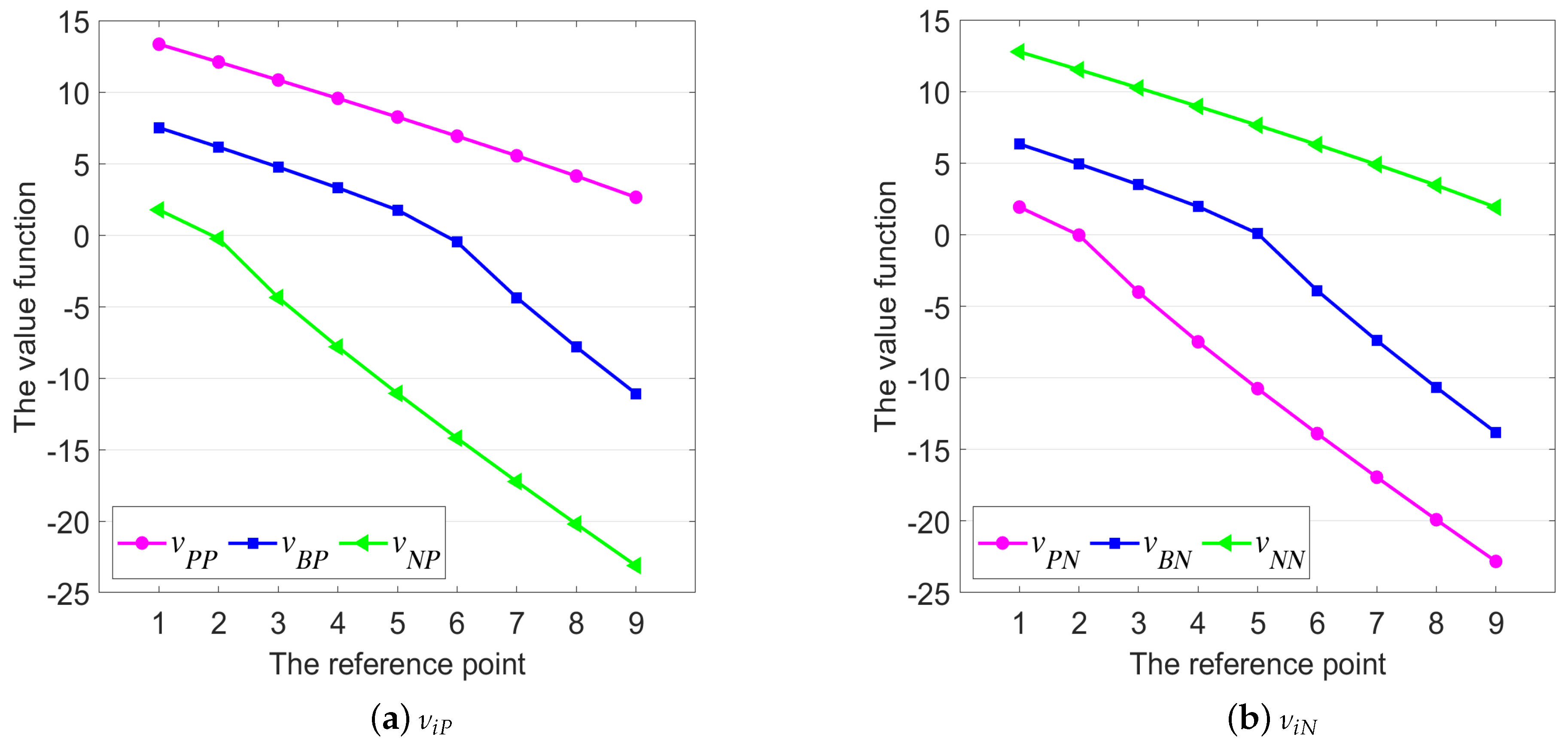
A venture capital firm makes decisions $\mathcal{A}=\{a_P,a_B,a_N\}$ through the assessment of result $\Omega =\{X,\neg X\}$ by an expert, as shown in

Table 4. The outcome of the matrix.

	X	$\neg \mathit{X}$
$a_P$	$[6.69,9.31]$	$[-10.18,-7.64]$
$a_B$	$[-1.59,-0.65]$	$[-3.32,-2.40]$
$a_N$	$[-10.35,-7.87]$	$[5.92,8.24]$

. The reference point ${\tilde{e}}_k$ represents the ideal return that the investment company wants to obtain. The expected return of nine different decision-makers is shown in

Table 5. The reference point expectations of the decision-maker.

The Reference Point	${\mathit{d}}_1$	${\mathit{d}}_2$	${\mathit{d}}_3$	${\mathit{d}}_4$	${\mathit{d}}_5$	${\mathit{d}}_6$	${\mathit{d}}_7$	${\mathit{d}}_8$	${\mathit{d}}_9$
$m\left({\tilde{e}}_k\right)$	$-11$	$-9$	$-7$	$-5$	$-3$	$-1$	1	3	5

.

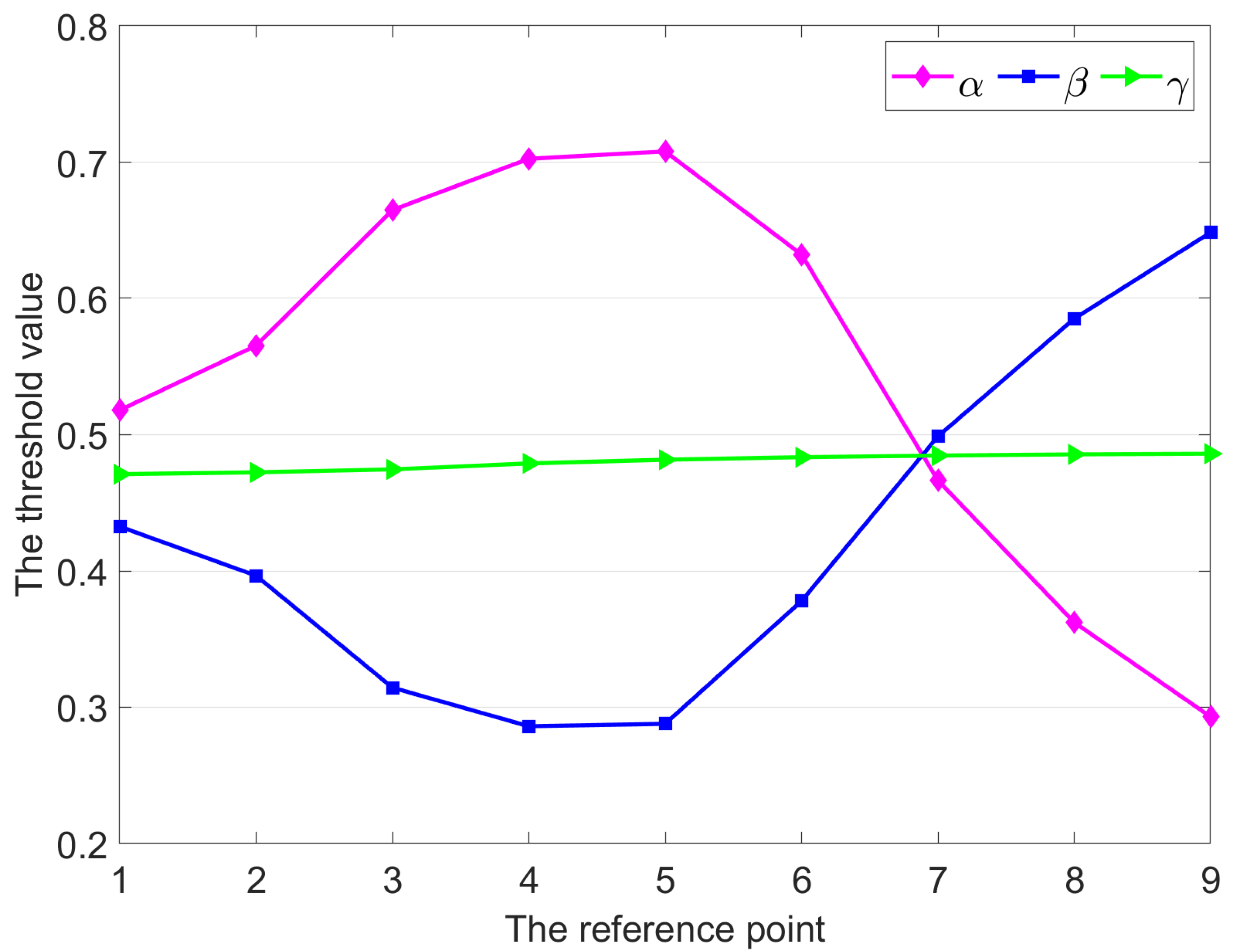
From Table 4, we can see that $0.46\le r\left({\tilde{x}}_{ij}\right)\le 1.27$ ($i=P,B,N,j=P,N$). In order to analyze the relationship between the expectation (i.e., risk attitude) of different decision-makers and the value function in Algorithm 1, the interval radius of nine decision makers is assumed to be $r\left({\tilde{e}}_k\right)=0.8$ ($k=1,2,\cdots ,9$). Figure 4 represents the decision prospect obtained by nine decision-makers taking decision actions under states ${\tilde{x}}_{ij}$, and Figure 5 represents the threshold values $\alpha$, $\beta$, and $\gamma$ obtained by nine decision-makers. It can be seen from Figure 4 that when the expectation value of the reference point of the decision-maker increases gradually, the decision prospect of adopting various decision actions decreases gradually, and ${\nu }_{NP}^k<{\nu }_{BP}^k\le {\nu }_{PP}^k$, ${\nu }_{PN}^k<{\nu }_{BN}^k\le {\nu }_{NN}^k$. When ${\nu }_{ij}<0$, the decline trend of the decision prospect is faster, which indicates that the decision-maker is more sensitive to the decision in the loss state in the decision process. As shown in Figure 5, $\alpha$ increases first and then decreases, $\beta$ decreases first and then increases, $\gamma$ has no obvious change trend, and $\alpha$, $\beta$ and $\gamma$ satisfy Proposition 5. When the reference point of the decision-maker is $d_7$, $d_8$, or $d_9$, we have $\alpha <\beta$, so the three-way decision is reduced to a two-way decision. In other words, when decision-makers have different ideal returns on investment results, investment companies have different requirements on the probability of investment success when choosing whether to invest funds according to decision-makers’ preferences.

5.2. Comparative Analysis

In order to reflect the influence of the interval value radius, we take $m\left({\tilde{e}}_5\right)$ as an example. Nine reference points with different radii were selected, in which the radii of the interval values were set as 0 initially, $0.4$ step and $3.2$ maximum value (i.e., $r\left({\tilde{e}}_5\right)=\left\{0.4s\right|s=0,1,2,\cdots ,8\}$). Then, the change in the prospect value function and threshold $(\alpha ,\beta )$ were analyzed. When ${\tilde{x}}_{ij}$ and ${\tilde{e}}_k$ are precise real numbers (i.e., ${\tilde{e}}_5=e_5^{-}=e_5^{+}$,${\tilde{x}}_{ij}=x_{ij}^{-}=x_{ij}^{+}$), the model proposed in this paper is reduced to the CPTWD model in Wang’s model [21]. In order to compare with Wang’s model, the location function in Definition 6 is used to convert the interval value in Table 4 into a real number, where $x=0.5$, for example, ${\tilde{x}}_{PP}=f_{\tilde{a}}\left(0.5\right)=x_{PP}^{-}+(x_{PP}^{+}-x_{PP}^{-})x=8$.

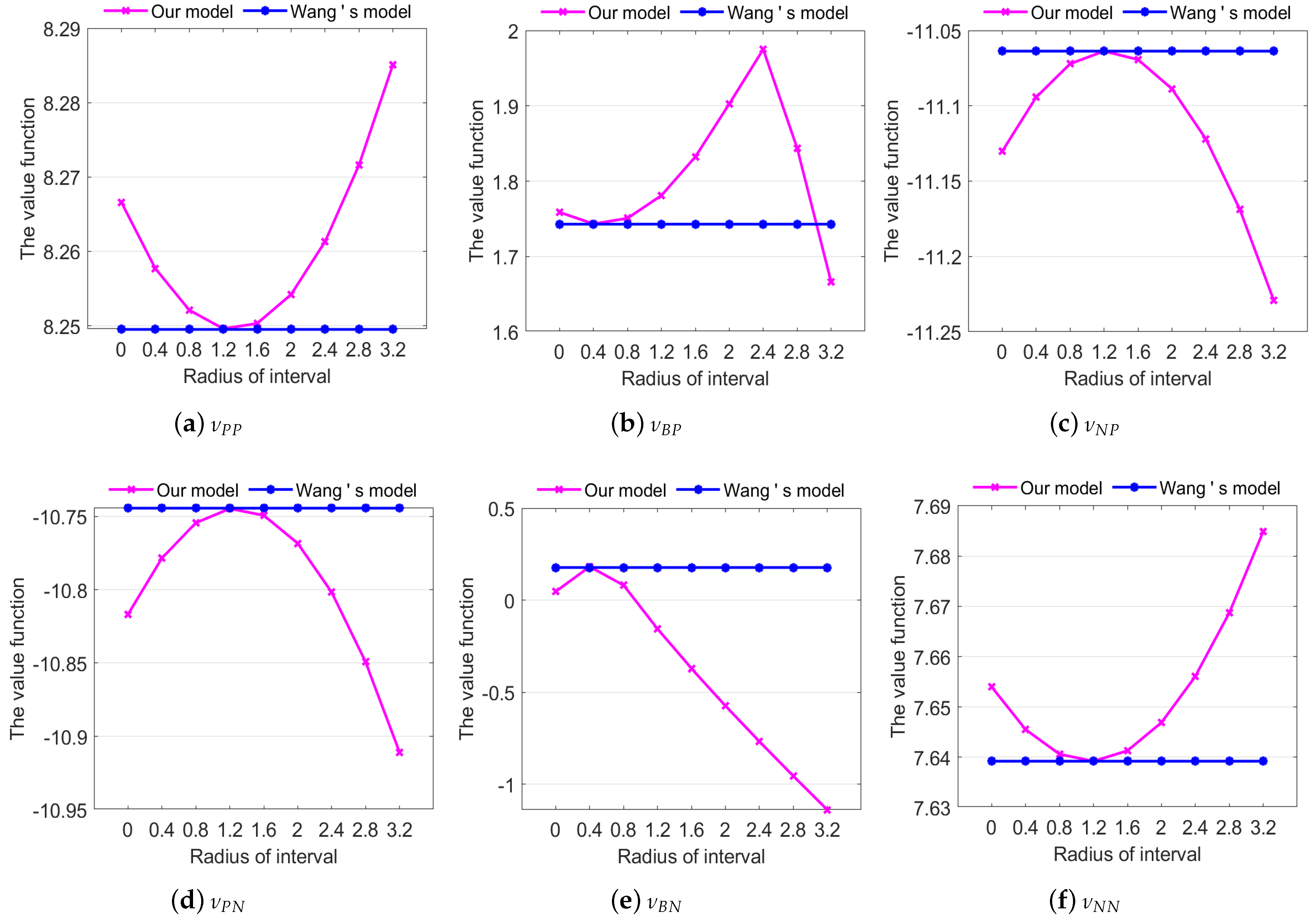
When the reference point radius changes, the corresponding prospect value function is obtained by the fifth decision-maker who takes decision action under the state ${\tilde{x}}_{ij}$ is shown in Figure 6. It can be seen from Figure 6 that ${\nu }_{ij}$ in Wang’s model is not affected by the radius of the reference point $r\left({\tilde{e}}_5\right)$. Since $r\left({\tilde{x}}_{PP}\right)=1.31$, $|r\left({\tilde{x}}_{PP}\right)-r\left({\tilde{e}}_5\right)|$ reaches the minimum value when $r\left({\tilde{e}}_5\right)=1.2$. As shown in Figure 6a, the difference in the prospect value function between our model and Wang’s model is minimal when $r\left({\tilde{e}}_5\right)=1.2$. This indicates that when the radius difference between ${\tilde{x}}_{PP}$ and ${\tilde{e}}_5$ is the smallest, their prospect value function is the closest. Similarly, the analysis shows that Figure 6b–f have the same results as Figure 6a. Due to the fact that $e_5^{+}=m\left({\tilde{e}}_5\right)+r\left({\tilde{e}}_5\right)=-3+r\left({\tilde{e}}_5\right)\le -3+0.4\times 8=0.2$, $e_5^{-}=m\left({\tilde{e}}_5\right)-r\left({\tilde{e}}_5\right)=-3-r\left({\tilde{e}}_5\right)\le -3-0.4\times 8=-0.62$, we have $x_{PP}^{-}=6.91>0.2>e_5^{+}$, $x_{NP}^{+}=-7.87<-6.2<e_5^{-}$, $x_{PN}^{+}=-7.64<-6.2<e_5^{-}$, $x_{NN}^{-}=5.92>0.2>e_5^{+}$. Therefore, the relationship between ${\tilde{x}}_{PP}$, ${\tilde{x}}_{NP}$, ${\tilde{x}}_{PN}$, ${\tilde{x}}_{NN}$, and ${\tilde{e}}_5$ is not always inclusive when $r\left({\tilde{e}}_5\right)=\left\{0.4s\right|s=0,1,2,\cdots ,8\}$. As shown in Figure 6a,c,d,f, when $|r\left({\tilde{x}}_{ij}\right)-r\left({\tilde{e}}_5\right)|$ is larger, the difference between the prospect value function of our model and Wang’s model is larger. In other words, the difference in the prospect value function of our model and Wang’s model is positively correlated with the difference in radius of ${\tilde{x}}_{ij}$ and ${\tilde{e}}_5$ if the relationship between ${\tilde{x}}_{ij}$ and ${\tilde{e}}_5$ is not inclusive.

Since ${\tilde{x}}_{BP}=[-1.59,-0.65]$, we have ${\tilde{x}}_{BP}\subset {\tilde{e}}_5$ when $r\left({\tilde{e}}_5\right)=2.4$ or $r\left({\tilde{e}}_5\right)=2.8$ or $r\left({\tilde{e}}_5\right)=3.2$. As shown in Figure 6, when $r\left({\tilde{e}}_5\right)=2.4$ or $r\left({\tilde{e}}_5\right)=2.8$, the prospect value function of our model is greater than that of Wang’s model. When $r\left({\tilde{e}}_5\right)=3.2$, the prospect value function of our model is less than that of Wang’s model. Since ${\tilde{x}}_{BN}=[-3.32,-2.40]$, we have the following: if $r\left({\tilde{e}}_5\right)=0$, ${\tilde{e}}_5\subset {\tilde{x}}_{BN}$; if $r\left({\tilde{e}}_5\right)=0.4$ or $r\left({\tilde{e}}_5\right)=0.8$, the relationship between ${\tilde{x}}_{BN}$ and ${\tilde{e}}_5$ is not inclusive; if $r\left({\tilde{e}}_5\right)\ge 1.2$, ${\tilde{x}}_{BN}\subset {\tilde{e}}_5$. The difference in prospect value function of the two models is also positively correlated with the difference in radius of ${\tilde{x}}_{BN}$ and ${\tilde{e}}_5$. Combining Figure 6b,e, we find that the change in prospect value function is complex, if the relationship between ${\tilde{x}}_{ij}$ and ${\tilde{e}}_5$ is inclusive.

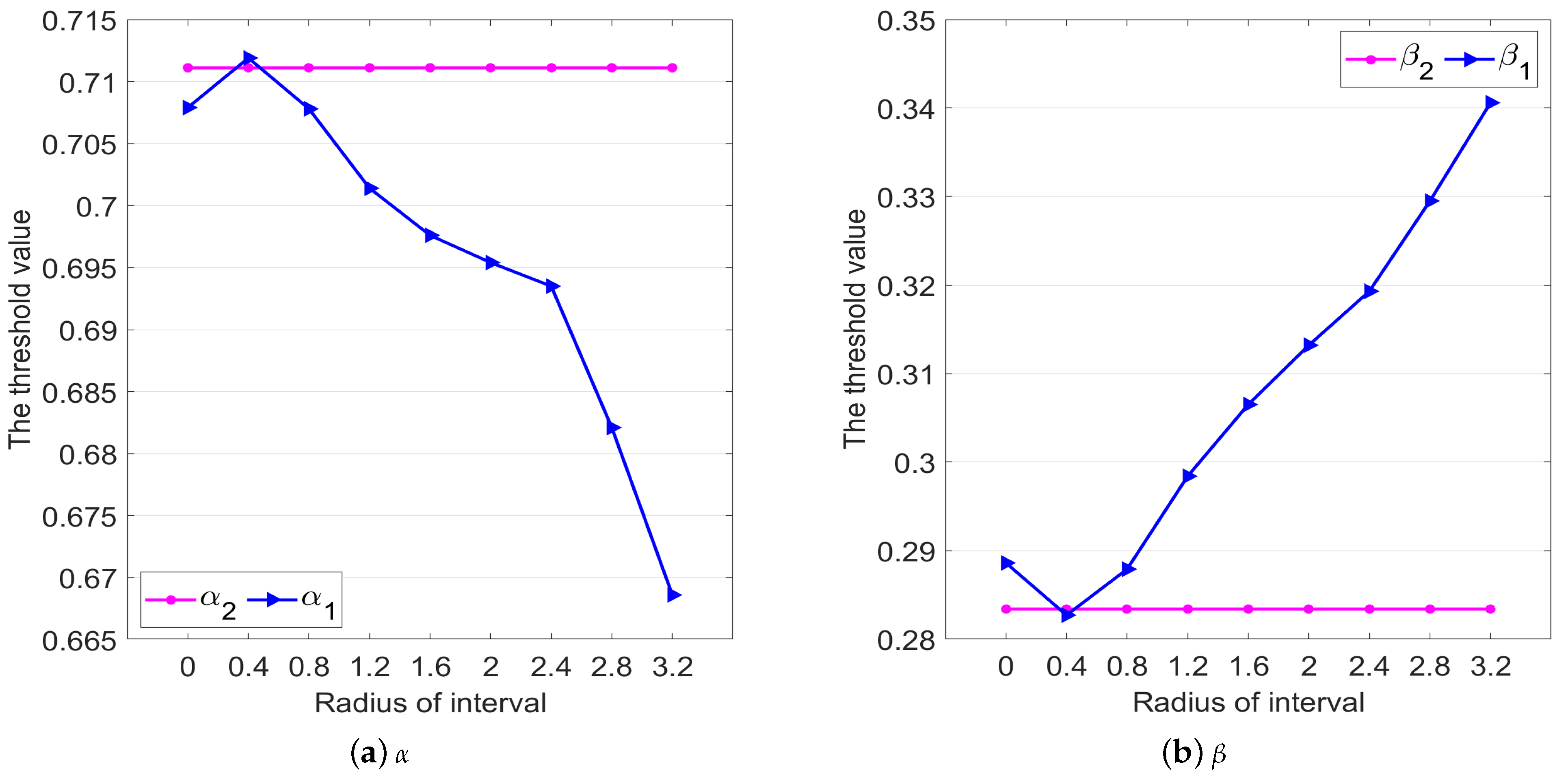
The thresholds $\alpha$ and $\beta$ are obtained under the difference radius of the reference point as shown in Figure 7, where ${\alpha }_1$ and ${\beta }_1$ represent the threshold obtained in this paper, and ${\alpha }_2$ and ${\beta }_2$ represent the threshold obtained in Wang’s. Ordinarily, the larger the interval radius, the larges the fluctuation range of the expected returns is. When $r\left({\tilde{e}}_5\right)=0.4$, the difference in thresholds between our model and Wang’s model is minimal. When $r\left({\tilde{e}}_5\right)>0.4$, ${\alpha }_1$ gradually decreases and ${\beta }_1$ gradually increases, while Wang’s is not affected.

Compared with Wang’s model, the proposed model has the following advantages:

(1).

While reflecting the preference of decision-makers, it fully considers the uncertainty of decision information in real life.

(2).

On the decision-making process, the fluctuation range of reference points is fully considered, that is, the acceptable range of decision-makers when they bear risk losses. The larger the interval radius is, the larger the fluctuation range of expected returns is. However, because the data used by Wang’s model are precise, they cannot reflect the influence of the interval radius of reference points on decision-making behavior.

(3).

This method can accurately judge the loss and gain state after taking the decision when there is an inclusion relation between the reference point and the outcome.

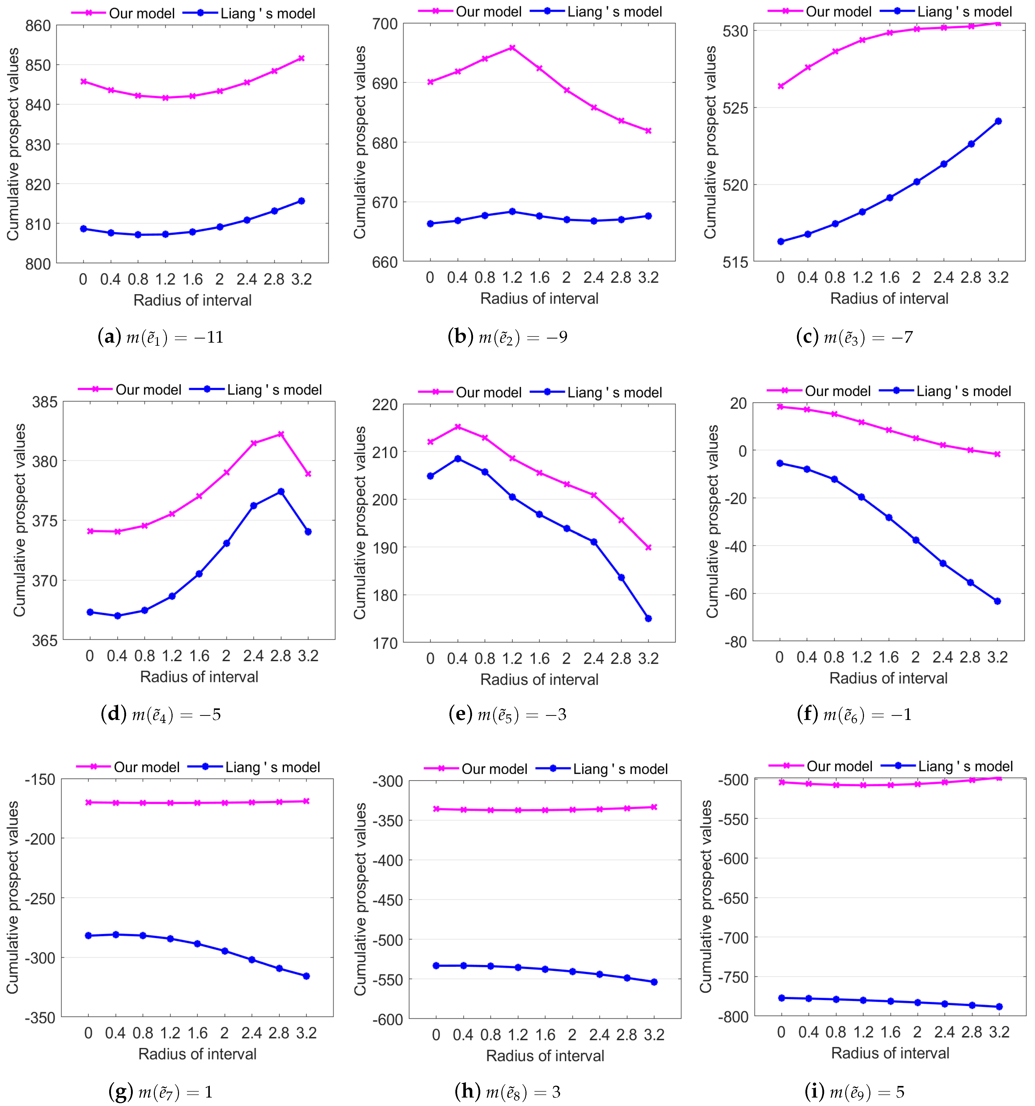
For the treatment of interval value, reference [33] deduces a three-way decision model based on IVDTRS with a certain ranking method (hereinafter referred to as Liang’s model). In this model, Liang first gives the transformation formula of $m_{\theta }\left(\tilde{\lambda }\right)=(1-\theta ){\lambda }^{-}+\theta {\lambda }^{+}$ ($\theta \in [0,1]$) and converts the loss function regarding the risk or cost of actions in the different states in IVDTRS into a real number. Then, the risk loss assessment is carried out on three different decision actions with the help of the Bayesian decision theory, and finally the decision action with the least expected loss as the final decision rule is selected. However, Wang’s model fails to reflect the attitudes of decision-makers toward the gain, while the method proposed in this paper could reflect the decision-makers’ preference. In order to show the superiority of our model in the decision prospect, we compare our model with Liang’s model. First, in Liang’s model, since risks are measured by the loss functions, the outcome matrix in Table 4 needs to be transformed into the loss function matrix. If $x_{ij}^{-}\ge 0$, the decision is in the gain state, so the loss function is set as ${\tilde{\lambda }}_{ij}=0$. If $x_{ij}^{+}\le 0$, the decision is in a loss state, the loss function is set as ${\tilde{\lambda }}_{ij}=[-x_{ij}^{+},-x_{ij}^{-}]$. For the selection of $\theta$ in $m_{\theta }\left(\tilde{\lambda }\right)$, we set the initial value of $\theta$ to 0, the step size to $0.125$, and the maximum to 1. Therefore, nine sets of $\alpha$, $\beta$, and $\gamma$ can be obtained by Liang’s model. The conditional probability $Pr\left(X\right|\left[o\right])$ takes 99 events from $0.01$ to $0.99$ with the step length of $0.01$. Thus, nine different decision rules can be obtained, respectively. Furthermore, the decision prospect value of each event can be calculated based on the decision rule, and then the total prospect value of all events can be obtained.

In order to illustrate the effectiveness, the largest decision prospect group among the nine groups of decision rules of Liang’s model is selected to be compared with the algorithm in this paper, as shown in Figure 8. Figure 6a represents the change in decision prospect values under the different radii of the reference point when $m\left({\tilde{e}}_1\right)=-11$, and the other eight sub-graphs are similar. It can be seen from Figure 8 that the decision prospect value of our model is always higher than that of Liang’s model. In addition, when the expectation of the reference point is the same, the decision prospect value under different radii of the reference point always changes.

Compared with Liang’s model, the proposed model has the following advantages:

(1).

Our model retains the uncertainty characteristic of the outcome matrix and discusses the risk attitude from the point of reference of decision-makers.

(2).

Decision-makers’ risk preference from the perspectives of loss and gain is reflected as risk aversion toward gains and risk-seeking toward losses.

(3).

The decision rules of Liang’s model are deduced based on the decision risk minimization principle, and only consider the losses in the decision-making process. According to the cumulative prospect value maximization, our model rules consider not only the loss but the gain.

6. Conclusions

In this paper, the cumulative prospect theory is introduced into the interval value three-way decision method, and a new three-way decision model is constructed. With the help of the distance measure between the two interval values, the loss function and gain function are analyzed under the uniform distribution state. Then, the effects of different reference points and decision-makers’ risk preference on the gains and losses is described in the light of the prospect theory. The probability weight is transformed into two weight functions about the gain and the loss. The existence and uniqueness of the threshold in our model are proved, and the decision rules are further simplified. Finally, the change in the prospect value and threshold value in different reference points is analyzed in the experiments. Furthermore, the traditional interval value processing method is compared with the algorithm in our paper, which shows that the algorithm in our paper can better reflect the preference of decision-makers. Comparing with IVDTRS, this shows that the proposed algorithm has better decision prospects. The proposed algorithm can effectively reflect the decision behavior of decision-makers. It is a useful extension of the interval-valued three-way decision model. However, there are still some deficiencies in our model. For example, in the construction of the loss function and the gain function, we assume that any value of the interval value is uniformly distributed. In fact, the uniformly distributed interval number is rare. Therefore, how to reasonably integrate the calculation methods of probability distribution function and prospect value function is the next research focus.

References

- Yao, Y.Y. Three-way decsions with probabilistic rough sets. Inf. Sci. 2009, 180, 341–353. [Google Scholar] [CrossRef] [Green Version]
- Li, W.Z.; Gao, P.X.; Chen, J.; Lu, Y.Q. UAV situation assessment based on cumulative prospect theory and three-way decision. J. Shanghai Jiaotong Univ. 2021, 1–12. [Google Scholar] [CrossRef]
- Wen, H.; Yang, B. Intelligent decision system for urban rail transit turnout regulation based on abnormal granularity and three-way decision theory. Urban Rail Transit Res. 2021, 24, 136–145. [Google Scholar]
- Yue, X.D.; Liu, S.W.; Yuan, B. Three-way decision of medical image based on neural network of depth of evidence. J. Northwest Univ. (Natural Sci. Ed.) 2021, 51, 539–548. [Google Scholar]
- Chen, Z.J.; Yan, R.X.; Peng, L.G. RFM customer segmentation model based on three-way decision rough set. Comput. Digit. Eng. 2020, 48, 361–366+371. [Google Scholar]
- Liu, D.; Yao, Y.Y.; Li, T.R. Three-way decision rough sets. Comput. Sci. 2011, 38, 246–250. [Google Scholar]
- Xu, J.F.; He, Y.F.; Liu, L. Research on the relationship and reasoning of cost objective function of three-way decision. Comput. Sci. 2018, 45, 176–182. [Google Scholar]
- Xie, Q.; Zhang, Q.H.; Wang, G.Y. Adaptive three-way spam filter based on similarity measure. Comput. Res. Dev. 2019, 56, 2410–2423. [Google Scholar]
- Chen, G.; Liu, B.Q.; Wu, Y. A new algorithm for optimal threshold of three-way decision. Comput. Appl. 2012, 32, 2212–2215. [Google Scholar]
- Jia, X.Y.; Shang, L.A. simulated annealing algorithm for three-way decision threshold. Small Microcomput. Syst. 2013, 34, 2603–2606. [Google Scholar]
- Zhang, N.; Jiang, L.L.; Yue, X.D.; Zhou, J. Utility three-way decision model. J. Intell. Syst. 2016, 11, 459–468. [Google Scholar]
- Kahneman, D.; Tversky, A. Prospec theory: An analysis of decision under risk. Econometrica 1979, 47, 263–291. [Google Scholar] [CrossRef] [Green Version]
- Yang, Y.P.; Lei, Z.J.; Lan, C.X.; Wang, X.R.; Gong, Z. Multi-stage decision-making method for product industrial design based on Bayesian network and prospect theory. Acta Graph. Sin. 2022, 43, 537–547. [Google Scholar]
- Yan, M.T.; Zhang, Q.; Jiang, K.X. Research on multiple attribute decision making method based on prospect theory. Comput. Knowl. Technol. 2020, 16, 1–2+8. [Google Scholar]
- Xue, Z.A.; Pang, W.L.; Yao, S.Q. Direct fuzzy three-way decision model based on prospect theory. J. Henan Norm. Univ. (Natural Sci. Ed.) 2022, 48, 2+31–36+79. [Google Scholar]
- Hu, Y.; Chen, H.Y. Emergency group decision-making model of network public opinion based on three-way decision and prospect theory. J. Anhui Univ. (Natural Sci. Ed.) 2020, 44, 13–19. [Google Scholar]
- Tversky, A.; Kahneman, D. Advances in prospect theory: Representation of cumulative uncertainty. J. Risk Uncertain. 1992, 5, 297–323. [Google Scholar] [CrossRef]
- Chang, J.; Du, Y.X.; Liu, W.F. Pythagorean hesitant fuzzy risk type multi-attribute decision making method based on cumulative prospect theory and VIKOR. Oper. Res. Manag. 2022, 31, 50–56. [Google Scholar]
- Wang, X.H.; Wang, B.; Liu, S.; Li, H.X.; Wang, T.X.; Watada, J. Fuzzy portfolio selection based on three-way decision and cumulative prospect theory. Int. J. Mach. Learn. Cybern. 2022, 13, 293–308. [Google Scholar] [CrossRef]
- Wang, T.X.; Li, H.X.; Zhou, X.Z.; Huang, B.; Zhu, H.B. A prospect theory-based three-way decision model. Knowl. Based Syst. 2020, 203, 106–129. [Google Scholar] [CrossRef]
- Wang, T.X.; Li, H.X.; Zhang, L.B.; Zhou, X.Z.; Huang, B. A three-way decision model based on cumulative prospect theory. Inf. Sci. 2020, 519, 74–92. [Google Scholar] [CrossRef]
- Yin, D.L.; Cui, G.H.; Huang, X.Y.; Zhang, H. Interval pythagorean fuzzy multiple attribute decision making based on improved score function and prospect theory. Syst. Eng. Electron. Technol. 2022, 1–11. [Google Scholar] [CrossRef]
- Hu, J.H.; Xu, Q. Multi-criteria decision method for interval-valued based on prospect theory. J. Stat. Inf. 2011, 26, 23–27. [Google Scholar]
- Xiong, N.X.; Wang, Y.M. Interval grey number multiple attribute decision making based on prospect theory and evidential reasoning. Comput. Syst. Appl. 2019, 28, 33–40. [Google Scholar]
- Fan, Z.P.; Zhang, X.; Chen, F.D.; Liu, Y. Multiple attribute decision making considering aspiration-levels: A method based on prospect theory. Comput. Ind. Eng. 2013, 65, 341–350. [Google Scholar] [CrossRef]
- Wang, T.X.; Li, H.X.; Zhou, X.Z.; Liu, D.; Huang, B. Three-way decision based on third-generation prospect theory with Z-numbers. Inf. Sci. 2021, 569, 13–38. [Google Scholar] [CrossRef]
- Tran, L.; Duckstein, L. Multiobjective fuzzy regression with central tendency and possibilistic properties. Fuzzy Sets Syst. 2002, 130, 21–31. [Google Scholar] [CrossRef]
- Moore, R.; Lodwick, W. Interval analysis and fuzzy set theory. Fuzzy Sets Syst. 2003, 135, 5–9. [Google Scholar] [CrossRef]
- Bao, Y.E.; Peng, X.Q.; Zhao, B. Interval number distance based on expectation and width and Its completeness. Fuzzy Syst. Math. 2013, 27, 133–139. [Google Scholar]
- Liu, D.; Li, T.R.; Li, H.X. Rough set theory: A three-way decision erspective. J. Nanjing Univ. (Natural Sci. Ed.) 2013, 49, 574–581. [Google Scholar]
- Liu, D.; Liang, D.C.; Wang, C.C. A novel three-way decision model based on incomplete information system. Knowl. Based Syst. 2016, 91, 32–45. [Google Scholar] [CrossRef]
- Liu, D.; Li, T.R.; Li, H.X. Interval decision rough sets. Comput. Sci. 2012, 39, 178–181+214. [Google Scholar]
- Liang, D.C.; Liu, D. Systematic studies on three-way decisions with interval-valued decision-theoretic rought sets. Inf. Sci. 2014, 276, 186–203. [Google Scholar] [CrossRef]
- Xu, Y.; Wang, X.S. Three-way decision based on improved aggregation method of interval loss function. Inf. Sci. 2020, 508, 214–233. [Google Scholar] [CrossRef]
- Li, Y.; Zhang, D.X. Multi-attribute grey target decision-making method under three-parameter interval grey number information based on prospect theory. Henan Sci. 2018, 36, 1001–1008. [Google Scholar]
- Ci, T.J. Research on interval number multiple attribute decision making method based on decision makers preference. Hebei Univ. Technol. 2014. [Google Scholar] [CrossRef]
Figure 1.
The value function.
Figure 2.
The weight function.
Figure 3.
The location function.
Figure 4.
The trend of the value function.
Figure 5.
The trend of threshold change.
Figure 6.
Comparison of value functions of different interval radii.
Figure 7.
Comparison of threshold values of different interval radii.
Figure 8.
Comparison of decision prospect values of different risk attitudes.