The Harris Extended Bilal Distribution with Applications in Hydrology and Quality Control

Abstract

In this research work, a new three-parameter lifetime distribution is introduced and studied. It is called the Harris extended Bilal distribution due to its construction from a mixture of the famous Bilal and Harris distributions, resulting from a branching process. The basic properties, such as the moment generating function, moments, quantile function, and Rényi entropy, are discussed. We show that the hazard rate function has ideal features for modeling increasing, upside-down bathtub, and roller-coaster data sets. In a second part, the Harris extended Bilal model is investigated from a statistical viewpoint. The maximum likelihood estimation is used to estimate the parameters, and a simulation study is carried out. The flexibility of the proposed model in a hydrological data analysis scenario is demonstrated using two practical data sets and compared with important competing models. After that, we establish an acceptance sampling plan that takes advantage of all of the features of the Harris extended Bilal model. The operating characteristic values, the minimum sample size that corresponds to the maximum possible defects, and the minimum ratios of lifetime associated with the producer’s risk are discussed.

1. Introduction

Modern data are diverse and complex, so new statistical models based on appealing distributions have long been popular in the statistical literature. Among the most notable references, the authors in [1] introduced a new one-parameter distribution known as the Bilal distribution, which yields more flexibility in the modeling of real data sets than the exponential and Lindley distributions. Although the Bilal distribution has received less attention, there has been great interest in its extensions, generalizations, and related applications. A short retrospective on this topic is offered below. A two-parameter generalization was introduced in [2] as a solution to the unimodal hazard rate function (hrf) of the Bilal distribution. The authors in [3] suggested that the scale parameter involved should be estimated using U-statistics. The log-Bilal distribution and associated regression, which provide better modeling of extremely skewed dependent variables with associated covariates, were introduced in [4]. In addition, the author in [5] proposed a new distribution based on the Poisson–Bilal distribution to model count data regression. The corresponding INAR(1) process for over-dispersed count data sets was also provided. The authors in [6] introduced the Farlie–Gumbel–Morgenstern bivariate Bilal distribution and its inferential aspects using concomitant order statistics. Some properties and an estimation under ranked set sampling were established for the generalized Bilal distribution in [7]. These studies have demonstrated the versatility of the Bilal distribution. There is, however, room for improvement in reaching the goal of perfect statistical modeling.

As a matter of fact, the extended distributions proposed by adding additional parameters generally provide an improved flexibility. To that end, the Harris extended family of distributions was introduced in [8] by modifying the baseline distribution with two parameters. A physical interpretation at the heart of this family is as follows: if a device is made up of N serial components with a fixed failure rate, where N is a random variable, then the Harris extended family is defined by the distribution of the device’s time until failure. Thus, it results from a branching process. More information on this construction can be found in [9]. The Harris extended family can also be viewed as a generalization of the Marshall–Olkin distribution developed in [10], with an additional new parameter providing more control over the distribution’s shape. It provides an adequate model in various research fields, such as hydrology, insurance, biology, and life testing.

The new lifetime distributions have a large amount of room for quality control because of the non-standard lifetime data scenarios. In this context, acceptance sampling plans (ASPs) play a major role. Due to certain restrictions, examining the whole production unit is impossible. Thus, the ASP acts as a decision rule for the acceptance of a lot from a sample of products. It arose from the consideration of both consumer and producer risks, representing a middle ground between complete inspection and no inspection.

The goal of this paper is to introduce the Harris extended Bilal (HEB) distribution, a three-parameter generalization of the Bilal distribution based on the idea in [8]. We emphasize its practical usefulness. In addition, we intend to compare the proposed distribution with the Harris extended Lindley (HEL) distribution proposed in [11] and the Harris extended exponential (HEE) distribution introduced in [12]. This is demonstrated through hydrological data analysis. We also propose the ASP, a reliability test plan for accepting or rejecting lots, where the lifetime of the product follows the HEB distribution and discusses its properties.

The remaining part of the paper is organized in the following order: Section 2 describes the nature of the probability density function (pdf) and hrf of the HEB distribution. In Section 3, we describe its associated statistical properties, such as the moment generating function (mgf), moments, quantile function, and (Rényi) entropy. The estimation of the parameters and the Fisher information matrix are discussed in Section 4. The large sample behavior of the HEB distribution, with the help of certain simulated data sets, is detailed in Section 5. In Section 6, two real data sets are analyzed using the proposed distribution. Section 7 investigates the ASP with a lifetime following the HEB distribution. Finally, the study is concluded in Section 8.

2. The Harris Extended Bilal Distribution

In this section, we describe the HEB distribution and elucidate some of its statistical properties.

As suggested in [8], assume that $X_1,X_2,\dots$ is a sequence of independent and identically distributed (iid) random variables with the pdf $f_1\left(x\right)$ and the survival function (sf) ${\overline{F}}_1\left(x\right)$. Consider a positive integer random variable N, independent of $X_1,X_2,\dots$, following the Harris distribution with parameters $\theta >0$ and $\delta >0$.

Let $X=min(X_1,X_2,\dots ,X_N)$. Then, the resulting distribution of X is known as the Harris extended family of distributions with sf of the form

$${\overline{G}}_{HE}\left(x\right)=\frac{{\theta }^{\frac{1}{\delta }}{\overline{F}}_1\left(x\right)}{{\left[1-\overline{\theta }{{\overline{F}}_1\left(x\right)}^{\delta }\right]}^{\frac{1}{\delta }}},x\in \mathbb{R},$$

(1)

where $\overline{\theta }=1-\theta$. Thus, $\theta$ and $\delta$ are the shape parameters, providing additional flexibility to the baseline sf ${\overline{F}}_1\left(x\right)$. The corresponding pdf is indicated as follows:

$$g_{HE}\left(x\right)=\frac{{\theta }^{\frac{1}{\delta }}{f}_1\left(x\right)}{{\left[1-\overline{\theta }{{\overline{F}}_1\left(x\right)}^{\delta }\right]}^{1+\frac{1}{\delta }}},x\in \mathbb{R}.$$

It can be considered as a generalization of the Marshall–Olkin family of distributions in [10], obtained by taking $\delta =1$ in (1).

On the other hand, the author in [1] introduced the Bilal distribution as a new one-parameter lifetime distribution with the following pdf:

$$f(x;\lambda )=\frac{6}{\lambda }\left(e^{-\frac{2x}{\lambda }}-e^{-\frac{3x}{\lambda }}\right),x>0,$$

and the following sf:

$$\overline{F}(x;\lambda )=3e^{-\frac{2x}{\lambda }}-2e^{-\frac{3x}{\lambda }},x>0,$$

where $\lambda >0$ is the scale parameter. It is understood that $f(x;\lambda )=0$ and $\overline{F}(x;\lambda )=1$ for $x\le 0$. Based on the mathematical material above, the proposition below gives the exact definition of the HEB distribution.

Proposition 1.

A continuous random variable X is said to follow the HEB distribution if its pdf and sf are given by

$$g(x;\lambda ,\theta ,\delta )=\frac{6{\theta }^{\frac{1}{\delta }}\left(e^{-\frac{2x}{\lambda }}-e^{-\frac{3x}{\lambda }}\right)}{\lambda {\left[1-\overline{\theta }{\left(3e^{-\frac{2x}{\lambda }}-2e^{-\frac{3x}{\lambda }}\right]}^{\delta }\right)}^{1+\frac{1}{\delta }}},x>0$$

(2)

and

$$\overline{G}(x;\lambda ,\theta ,\delta )=\frac{{\theta }^{\frac{1}{\delta }}\left(3e^{-\frac{2x}{\lambda }}-2e^{-\frac{3x}{\lambda }}\right)}{{\left[1-\overline{\theta }{\left(3e^{-\frac{2x}{\lambda }}-2e^{-\frac{3x}{\lambda }}\right)}^{\delta }\right]}^{\frac{1}{\delta }}},x>0,$$

(3)

respectively, where $\lambda >0$ is the scale parameter, $\theta >0$ and $\delta >0$ are the shape parameters, and $\overline{\theta }=1-\theta$. It is understood that $g(x;\lambda ,\theta ,\delta )=0$ and $\overline{G}(x;\lambda ,\theta ,\delta )=1$ for $x\le 0$.

Proof. 

The result is trivial since it can be obtained by substituting ${\overline{F}}_1\left(x\right)$ for $\overline{F}(x;\lambda )$ in (1). □

To specify the parameters, the HEB distribution will eventually be denoted as HEB($\lambda ,\theta ,\delta$). Two special cases of the HEB distribution emerged:

• The Marshall–Olkin Bilal (MOB) distribution when $\delta =1$ (literature to be discussed).
• The Bilal distribution when $\theta =1$.

The following theorem elucidates the convenient infinite series expansion of the pdf of the HEB distribution.

Theorem 1.

The pdf of the HEB distribution can be expressed in terms of simple exponential functions as

$$g(x;\lambda ,\theta ,\delta )=\sum _{i,j=0}^{\infty }{z}_{i,j}{e}^{-[j+2(1+\delta i)]\frac{x}{\lambda }}\left(1-e^{-\frac{x}{\lambda }}\right),x>0,$$

where

$$\begin{array}{c}\hfill z_{i,j}=w_i{3}^{\delta i-j}\left(\genfrac{}{}{0pt}{}{\delta i}{j}\right){(-1)}^j{2}^j,\end{array}$$

(4)

and

$$\begin{array}{ccc}\hfill w_i& =& \left\{\begin{array}{cc}{\displaystyle \left(\genfrac{}{}{0pt}{}{-({\delta }^{-1}+1)}{i}\right){(-1)}^i{\overline{\theta }}^i\frac{6}{\lambda }{\theta }^{\frac{1}{\delta }}}\hfill & if0<\theta <1\hfill \\ \\ {\displaystyle \frac{6}{\lambda \theta }{(-1)}^i\left[\sum _{l=i}^{\infty }{\left(\frac{1}{\theta }-1\right)}^l\left(\genfrac{}{}{0pt}{}{l}{i}\right)\left(\genfrac{}{}{0pt}{}{-({\delta }^{-1}+1)}{l}\right)\right]}\hfill & if\theta >1\hfill \end{array}\right..\hfill \end{array}$$

We recall that $\left(\genfrac{}{}{0pt}{}{-r}{i}\right)=\frac{(-r)(-r-1)\dots (-r-i+1)}{\Gamma (i+1)}$ and $\left(\genfrac{}{}{0pt}{}{r}{i}\right)=\frac{\Gamma (r+1)}{\Gamma (i+1)\Gamma (r-i+1)}$ for $i>0$ and $r>0$, where $\Gamma \left(x\right)$ denotes the standard gamma function. (It is worth noting that $\theta =1$ is omitted voluntarily because it corresponds to the well-known Bilal distribution.)

In order not to weigh down the presentation, this proof (as well as all some future proofs) is given in Appendix A.

The main interest of Theorem 1 is in terms of functional approximation: for large enough M, we can efficiently approximate the sophisticated pdf $g(x;\lambda ,\theta ,\delta )$ to a manageable sum of simple exponential functions as

$$g(x;\lambda ,\theta ,\delta )\approx \sum _{i,j=0}^M{z}_{i,j}{e}^{-[j+2(1+\delta i)]\frac{x}{\lambda }}\left(1-e^{-\frac{x}{\lambda }}\right),x>0.$$

Some important statistical measures related to the HEB distribution can therefore be simply approximated, as developed later.

Using (2) and (3), the hrf of the HEB distribution is given by

$$h(x;\lambda ,\theta ,\delta )=\frac{6(1-e^{-\frac{x}{\lambda }})}{\lambda \left(3-2e^{-\frac{x}{\lambda }}\right)\left[1-\overline{\theta }{\left(3e^{-\frac{2x}{\lambda }}-2e^{-\frac{3x}{\lambda }}\right)}^{\delta }\right]},x>0.$$

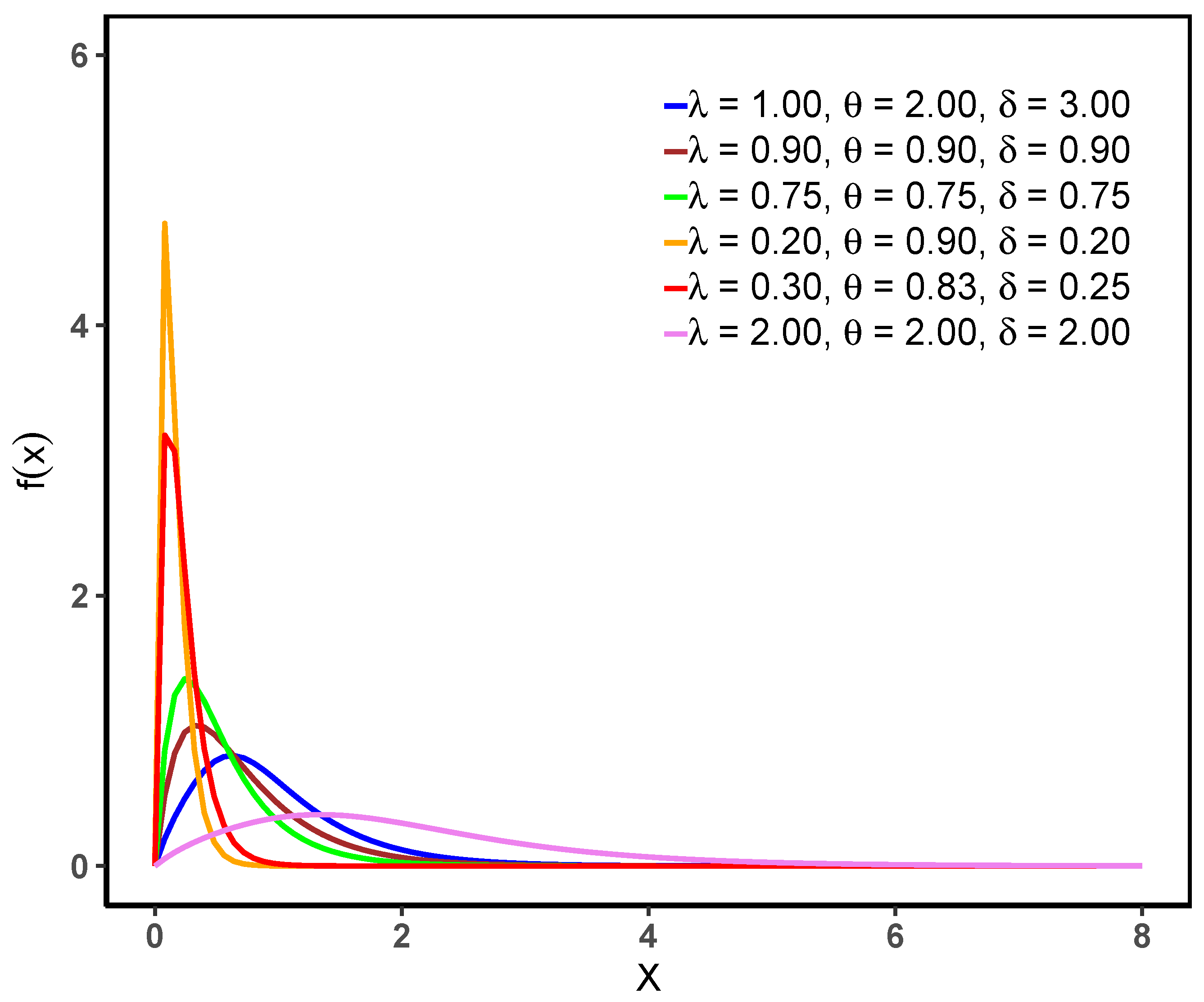
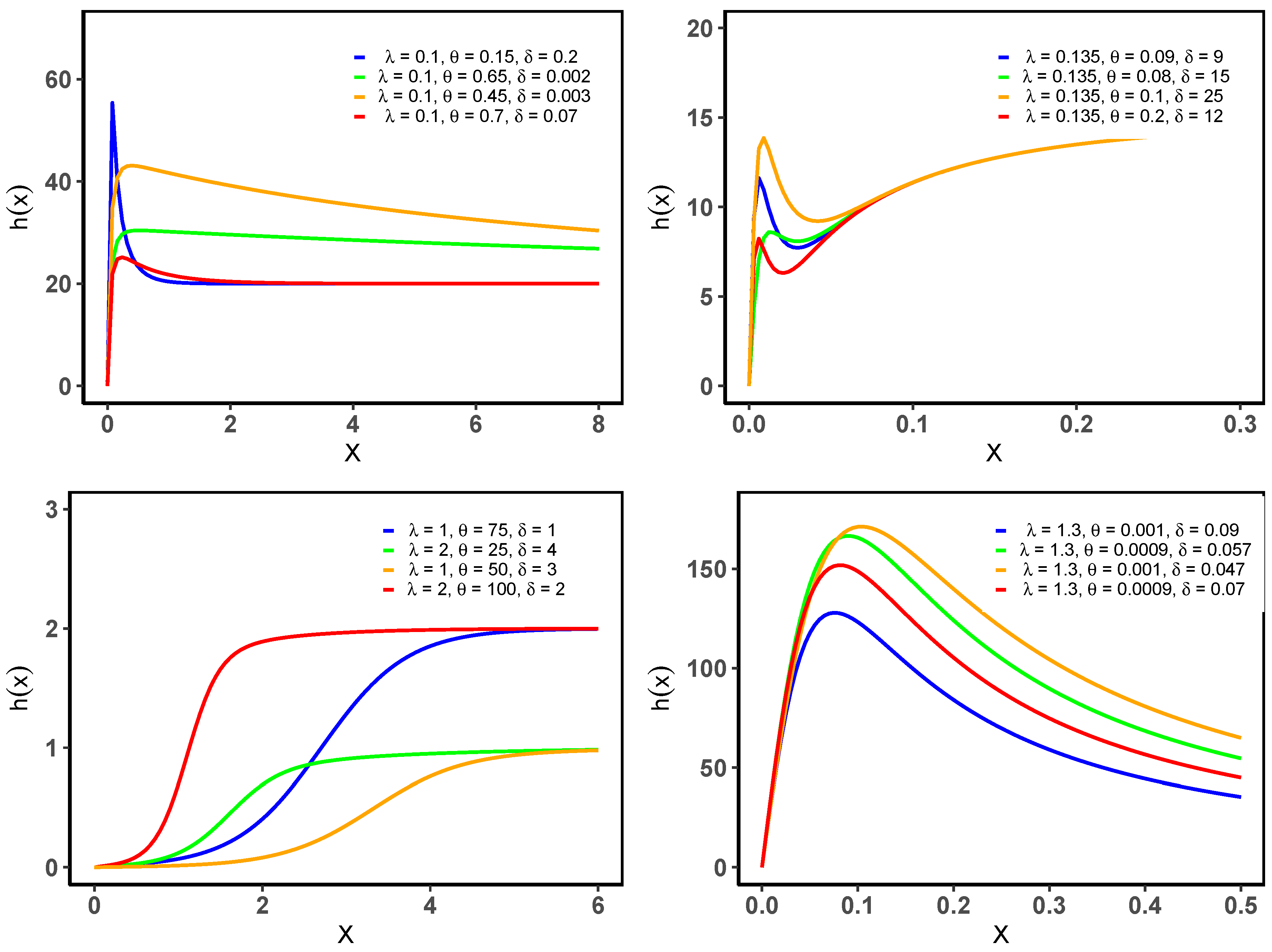
It is understood that $h(x;\lambda ,\theta ,\delta )=0$ for $x\le 0$. Figure 1 and Figure 2 display the pdf and hrf of the HEB distribution for different parameter values, respectively.

From Figure 1, we can see that the pdf is unimodal and right-skewed. Figure 2 shows that the hrf can be increasing (IFR), upside-down bathtub (UBT), and roller-coaster, which is not shared by the general Bilal (GB) distribution (see [2]).

3. Statistical Properties

In this section, some mathematical properties of the HEB distribution are intended for comparison because of the structural complexity of the Harris extended family of distributions.

3.1. Moment Generating Function and Moments

The next result presents a series expansion of the mgf of the HEB distribution.

Proposition 2.

Let X be a random variable following the HEB distribution. Then, the mgf of X is given by $M\left(t\right)=E\left(e^{tX}\right)$, and can be expressed as

$$M\left(t\right)=\sum _{i,j=0}^{\infty }{z}_{i,j}\frac{\lambda }{[j+2(1+\delta i)-\lambda t](j+3+2\delta i-\lambda t)},t<\frac{2}{\lambda }.$$

Proof. 

From the expansion in Theorem 1 and integration, we obtain

$$M\left(t\right)=\sum _{i,j=0}^{\infty }{z}_{i,j}{\int }_0^{\infty }{e}^{-[j+2(1+\delta i)-\lambda t]\frac{x}{\lambda }}\left(1-e^{-\frac{x}{\lambda }}\right)dx.$$

Considering the change in variables, $v=e^{-\frac{x}{\lambda }}$, we obtain

$$M\left(t\right)=\sum _{i,j=0}^{\infty }{z}_{i,j}\lambda {\int }_0^1{v}^{j+2(1+\delta i)-\lambda t-1}\left(1-v\right)dv=\sum _{i,j=0}^{\infty }{z}_{i,j}\lambda B(j+2(1+\delta i)-\lambda t,2),$$

where $B(a,b)$ refers to the standard beta function, $B(a,b)={\int }_0^1{v}^{a-1}{(1-v)}^{b-1}dv$, with $a>0$ and $b>0$. Since $B(a,2)=\frac{1}{a(a+1)}$, we obtain the desired result. □

As usual, the mgf can serve to generate the raw moments of X, find bounds for some probability involving X into an event via the Markov inequality, or characterize the independence of several random variables following the HEB distribution.

The next result presents a comprehensive expansion of the raw moments of X.

Proposition 3.

Let X be a random variable following the HEB distribution and r be an integer. Then, the rth raw moment of X is given by ${\mu }_r^{{}^{\prime }}=E\left(X^r\right)$ and can be expressed as

$$\begin{array}{c}\hfill {\mu }_r^{{}^{\prime }}=\sum _{i,j=0}^{\infty }{z}_{i,j}{\lambda }^{r+1}r!\left(\frac{1}{{[j+2(1+\delta i)]}^{r+1}}-\frac{1}{{[1+j+2(1+\delta i)]}^{r+1}}\right),\end{array}$$

where $z_{i,j}$ is expressed in (4).

The derivation is given in Appendix B.

In particular, from Proposition 3, we can derive the first two raw moments of X as

$$\begin{array}{c}\hfill {\mu }_1^{{}^{\prime }}=\sum _{i,j=0}^{\infty }{z}_{i,j}{\lambda }^2\left(\frac{1}{{[j+2(1+\delta i)]}^2}-\frac{1}{{[1+j+2(1+\delta i)]}^2}\right)\end{array}$$

and

$$\begin{array}{c}\hfill {\mu }_2^{{}^{\prime }}=\sum _{i,j=0}^{\infty }{z}_{i,j}{\lambda }^{3}2\left(\frac{1}{{[j+2(1+\delta i)]}^3}-\frac{1}{{[1+j+2(1+\delta i)]}^3}\right),\end{array}$$

respectively. The variance and standard deviation follow immediately.

3.2. Quantile Function

The following proposition gives the quantile function of the HEB distribution.

Proposition 4.

The quantile function of the HEB distribution is given by $Q(u;\lambda ,\theta ,\delta )=F^{-1}(u;\lambda ,\theta ,\delta )$, and can be expressed as

$$Q(u;\lambda ,\theta ,\delta )=-\lambda \log \left[\gamma \right(u\left)\right],$$

where

$$\begin{array}{c}\hfill \gamma \left(u\right)=\left\{\begin{array}{cc}{\displaystyle 0.5+sin\left({\alpha }_u+\frac{\pi }{6}\right)}\hfill & if0<\alpha <0.5\hfill \\ {\displaystyle 0.5}\hfill & if\alpha =0.5\hfill \\ {\displaystyle 0.5-cos\left({\alpha }_u+\frac{\pi }{3}\right)}\hfill & if0.5<\alpha <1\hfill \end{array}\right.,\end{array}$$

$$\begin{array}{c}\hfill {\alpha }_u=\frac{1}{3}{tan}^{-1}\left(\frac{2\sqrt{\alpha (1-\alpha )}}{2\alpha -1}\right)\mathrm{and}\alpha =1-\frac{1-u}{{[\theta +\overline{\theta }{(1-u)}^{\delta }]}^{\frac{1}{\delta }}}.\end{array}$$

Proof. 

Using (3), we need to solve $1-\overline{G}(x;\lambda ,\theta ,\delta )=u$, which is equivalent to

$$\begin{array}{c}\hfill 1-\left(3e^{-\frac{2x}{\lambda }}-2e^{-\frac{3x}{\lambda }}\right)=1-\frac{1-u}{{[\theta +\overline{\theta }{(1-u)}^{\delta }]}^{\frac{1}{\delta }}}.\end{array}$$

The left term is the cumulative distribution function (cdf) of the Bilal distribution. Hence, the proof follows from the quantile function of the Bilal distribution (see ([1] Equation (7))).

Since the HEB distribution has a closed-form quantile function, it has a variate generation property, which is very useful in simulation studies. □

3.3. Entropy

Entropy is the measure of uncertainty about a random variable. The most common measure of uncertainty is the Rényi entropy. It is given in the following proposition in the context of the HEB distribution.

Proposition 5.

Let X be a random variable following the HEB distribution. Then, the Rényi entropy of X is given by $I_R={(1-v)}^{-1}log\left\{E\left[g{(X;\lambda ,\theta ,\delta )}^{v-1}\right]\right\}$, with $v>0$ and $v\ne 1$, and can be expressed as

$$\begin{array}{c}\hfill I_R={(1-v)}^{-1}log\left[\sum _{i,j=0}^{\infty }{z}_{i,j}^{\left(v\right)}\lambda B(j+2(v+\delta i),v+1)\right],\end{array}$$

where

$$z_{i,j}^{\left(v\right)}=w_i^{\left(v\right)}{3}^{\delta i-j}\left(\genfrac{}{}{0pt}{}{\delta i}{j}\right){(-1)}^j{2}^j$$

and

$$\begin{array}{c}\hfill w_i^{\left(v\right)}=\left\{\begin{array}{cc}{\displaystyle \left(\genfrac{}{}{0pt}{}{-v({\delta }^{-1}+1)}{i}\right){(-1)}^i{\overline{\theta }}^i\frac{6^v}{{\lambda }^v}{\theta }^{\frac{v}{\delta }}}\hfill & if0<\theta <1\hfill \\ \\ {\displaystyle \frac{6^v}{{\left(\lambda \theta \right)}^v}{(-1)}^i\left[\sum _{l=i}^{\infty }{\left(\frac{1}{\theta }-1\right)}^l\left(\genfrac{}{}{0pt}{}{l}{i}\right)\left(\genfrac{}{}{0pt}{}{-v({\delta }^{-1}+1)}{l}\right)\right]}\hfill & if\theta >1\hfill \end{array}\right..\end{array}$$

The derivation is given in Appendix C.

4. Parameter Estimation

Here, we estimate the unknown parameters of the HEB distribution using the maximum likelihood (ML), least squares (LS), and weighted least squares (WLS) methods. Through the use of a simulation study, the effectiveness of these methods is assessed.

4.1. Maximum Likelihood Estimation

Let n be a positive integer and $X_1,X_2,\dots ,X_n$ be n iid random variables, which constitutes a random sample of size n, from the HEB$(\lambda ,\theta ,\delta )$ distribution. Let $x_1,x_2,\dots ,x_n$ be observations of these random variables. From (2), the log-likelihood function is given by

$$\begin{array}{cc}\hfill log{L}_{(\lambda ,\theta ,\delta )}& =nlog\left(\frac{6{\theta }^{\frac{1}{\delta }}}{\lambda }\right)-\sum _{i=1}^n\frac{2x_i}{\lambda }+\sum _{i=1}^{n}log\left(1-e^{-\frac{x_i}{\lambda }}\right)\hfill \\ \hfill & -\frac{1+\delta }{\delta }\sum _{i=1}^{n}log\left[1-\overline{\theta }{\left(3e^{-\frac{2x_i}{\lambda }}-2e^{-\frac{3x_i}{\lambda }}\right)}^{\delta }\right].\hfill \end{array}$$

(5)

The ML estimates $\widehat{\lambda },\widehat{\theta }$, and $\widehat{\delta }$ of the parameters $\lambda ,\theta$, and $\delta$, respectively, are those maximizing $log{L}_{(\lambda ,\theta ,\delta )}$ with respect to $\lambda ,\theta$, and $\delta$. They may be obtained from the solution of the following equations:

$$\frac{\partial log{L}_{(\lambda ,\theta ,\delta )}}{\partial \lambda }=0,\frac{\partial log{L}_{(\lambda ,\theta ,\delta )}}{\partial \theta }=0,\frac{\partial log{L}_{(\lambda ,\theta ,\delta )}}{\partial \delta }=0,$$

where

$$\begin{array}{cc}\hfill \frac{\partial log{L}_{(\lambda ,\theta ,\delta )}}{\partial \lambda }& =-\frac{n}{\lambda }+\sum _{i=1}^n\frac{2x_i}{{\lambda }^2}-\sum _{i=1}^n\frac{x_i{e}^{-\frac{x_i}{\lambda }}}{(1-e^{-\frac{x_i}{\lambda }}){\lambda }^2}\hfill \\ \hfill & +\sum _{i=1}^n\frac{6(1+\delta )\overline{\theta }{x}_i{\left(3e^{-\frac{2x_i}{\lambda }}-2e^{-\frac{3x_i}{\lambda }}\right)}^{\delta -1}\left(e^{-\frac{2x_i}{\lambda }}-e^{-\frac{3x_i}{\lambda }}\right)}{{\lambda }^2\left[1-\overline{\theta }{\left(3e^{-\frac{2x_i}{\lambda }}-2e^{-\frac{3x_i}{\lambda }}\right)}^{\delta }\right]},\hfill \\ \hfill \frac{\partial log{L}_{(\lambda ,\theta ,\delta )}}{\partial \theta }& =\frac{n}{\delta \theta }-\frac{1+\delta }{\delta }\sum _{i=1}^n\frac{{[3e^{-\frac{2x_i}{\lambda }}-2e^{-\frac{3x_i}{\lambda }}]}^{\delta }}{1-\overline{\theta }{\left(3e^{-\frac{2x_i}{\lambda }}-2e^{-\frac{3x_i}{\lambda }}\right)}^{\delta }}\hfill \end{array}$$

and

$$\begin{array}{cc}\hfill \frac{\partial log{L}_{(\lambda ,\theta ,\delta )}}{\partial \delta }& =-\frac{nlog\left(\theta \right)}{{\delta }^2}-\frac{1}{{\delta }^2}\sum _{i=1}^{n}log\left[1-\overline{\theta }{\left(3e^{-\frac{2x_i}{\lambda }}-2e^{-\frac{3x_i}{\lambda }}\right)}^{\delta }\right]\hfill \\ \hfill & +\frac{1+\delta }{\delta }\sum _{i=1}^n\frac{\overline{\theta }log\left(3e^{-\frac{2x_i}{\lambda }}-2e^{-\frac{3x_i}{\lambda }}\right)}{{\left(3e^{-\frac{2x_i}{\lambda }}-2e^{-\frac{3x_i}{\lambda }}\right)}^{-\delta }-\overline{\theta }}.\hfill \end{array}$$

Since we cannot find the solution in explicit form when equating to zero, we would go for the direct maximization of (5) using numerical methods.

The inference analysis on the parameters can be performed using the underlying asymptotic properties of the random ML estimators. For the vector parameter estimate $\widehat{\varphi }=(\widehat{\lambda },\widehat{\theta },\widehat{\delta })$, assuming classical regularity conditions, the asymptotic distribution behind $\widehat{\varphi }$ is the trivariate normal $N_3(\varphi ,K^{-1})$ distribution, where $K^{-1}$ is the information matrix of the parameters, $K=-J_n$, and

$$J_n={\left.\left[\begin{array}{ccc}\frac{{\partial }^{2}log{L}_{(\lambda ,\theta ,\delta )}}{\partial {\lambda }^2}& \frac{{\partial }^{2}log{L}_{(\lambda ,\theta ,\delta )}}{\partial \lambda \partial \theta }& \frac{{\partial }^{2}log{L}_{(\lambda ,\theta ,\delta )}}{\partial \lambda \partial \delta }\\ \frac{{\partial }^{2}log{L}_{(\lambda ,\theta ,\delta )}}{\partial \theta \partial \lambda }& \frac{{\partial }^{2}log{L}_{(\lambda ,\theta ,\delta )}}{\partial {\theta }^2}& \frac{{\partial }^{2}log{L}_{(\lambda ,\theta ,\delta )}}{\partial \theta \partial \delta }\\ \frac{{\partial }^{2}log{L}_{(\lambda ,\theta ,\delta )}}{\partial \delta \partial \lambda }& \frac{{\partial }^{2}log{L}_{(\lambda ,\theta ,\delta )}}{\partial \delta \partial \theta }& \frac{{\partial }^{2}log{L}_{(\lambda ,\theta ,\delta )}}{\partial {\delta }^2}\end{array}\right]\right|}_{(\lambda ,\theta ,\delta )=(\widehat{\lambda },\widehat{\theta },\widehat{\delta })}.$$

4.2. Least and Weighted Least Squares Estimation

Let $X_{\left(1\right)},X_{\left(2\right)},\cdots ,X_{\left(n\right)}$ be the order statistics of $X_1,X_2,\dots ,X_n$, i.e., such that $P(X_{\left(1\right)}\le X_{\left(2\right)}\le \dots \le X_{\left(n\right)})=1$. Let $x_{\left(1\right)},x_{\left(2\right)},\dots ,x_{\left(n\right)}$ be observations of these random variables. By minimizing the following function with respect to $\lambda ,\theta$, and $\delta$, we obtain the LS estimates of the parameters:

$$\begin{array}{c}\hfill L{S}_{(\lambda ,\theta ,\delta )}=\sum _{i=1}^n{\left[1-\frac{{\theta }^{\frac{1}{\delta }}\left(3e^{-\frac{2x_{\left(i\right)}}{\lambda }}-2e^{-\frac{3x_{\left(i\right)}}{\lambda }}\right)}{{\left[1-\overline{\theta }{\left(3e^{-\frac{2x_{\left(i\right)}}{\lambda }}-2e^{-\frac{3x_{\left(i\right)}}{\lambda }}\right)}^{\delta }\right]}^{\frac{1}{\delta }}}-\frac{i}{n+1}\right]}^2.\end{array}$$

Similarly, the WLS estimates of the parameters $\lambda ,\theta$, and $\delta$ are obtained by minimizing the following function:

$$\begin{array}{c}\hfill WL{S}_{(\lambda ,\theta ,\delta )}=\sum _{i=1}^n\frac{{(n+1)}^2(n+2)}{i(n-i+1)}{\left[1-\frac{{\theta }^{\frac{1}{\delta }}\left(3e^{-\frac{2x_{\left(i\right)}}{\lambda }}-2e^{-\frac{3x_{\left(i\right)}}{\lambda }}\right)}{{\left[1-\overline{\theta }{\left(3e^{-\frac{2x_{\left(i\right)}}{\lambda }}-2e^{-\frac{3x_{\left(i\right)}}{\lambda }}\right)}^{\delta }\right]}^{\frac{1}{\delta }}}-\frac{i}{n+1}\right]}^2.\end{array}$$

5. Simulation

The performance of the HEB model is analyzed by means of a simulation study. The simulation is run with $N=1000$ replications for a sample of size of $n=50$, 100, 150, 200, and 250, and the following arbitrary choices of parameter values: $(\lambda =1.5,\theta =0.8,\delta =2),(\lambda =1.3,\theta =1.1,\delta =2.1)$, and $(\lambda =1.18,\theta =1.45,\delta =2)$. The parameter estimation is carried out by the ML, LS, and WLS methods, and the following quantities are computed:

• Average bias (Bias) of the parameters, given by the following formula:
  Bias${\displaystyle \left(\widehat{\alpha }\right)=\frac{1}{N}\sum _{i=1}^N({\widehat{\alpha }}_i-\alpha ),}$ where $\alpha \in \{\lambda ,\theta ,\delta \}$,
• Root mean square error (RMSE) of the parameters, given by the following formula:
  RMSE${\displaystyle \left(\widehat{\alpha }\right)=\sqrt{\frac{1}{N}\sum _{i=1}^N{({\widehat{\alpha }}_i-\alpha )}^2},}$ where $\alpha \in \{\lambda ,\theta ,\delta \}$.

The simulation result is displayed in

Table 1. Simulation results.

$\mathit{\lambda }=1.5,\mathit{\theta }=0.8,\mathit{\delta }=2$
	n	MLE			LSE			WLSE
		Estimate	Bias	RMSE	Estimate	Bias	RMSE	Estimate	Bias	RMSE
	50	1.5548	0.0548	0.4551	1.6060	0.1060	0.3637	1.5903	0.0903	0.3584
	100	1.5482	0.0482	0.3320	1.5483	0.0483	0.2449	1.5393	0.0393	0.2273
$\lambda$	150	1.5505	0.0505	0.2677	1.5380	0.0380	0.2034	1.5238	0.0238	0.1881
	200	1.5375	0.0375	0.2218	1.5196	0.0196	0.1600	1.5180	0.0180	0.1541
	250	1.5386	0.0386	0.2011	1.5200	0.0200	0.1592	1.5174	0.0174	0.1449
	50	1.0431	0.2431	0.8600	0.8595	0.0595	0.5013	0.9240	0.1240	0.6263
	100	0.9290	0.1290	0.5843	0.8342	0.0342	0.3843	0.8551	0.0551	0.3696
$\theta$	150	0.8257	0.0257	0.3729	0.8312	0.0312	0.3099	0.8455	0.0455	0.3042
	200	0.8358	0.0358	0.3072	0.8186	0.0186	0.2566	0.8315	0.0315	0.2620
	250	0.8052	0.0052	0.2505	0.8210	0.0210	0.2424	0.8228	0.0228	0.2306
	50	2.2408	0.2408	1.4854	2.0767	0.0767	0.2950	2.1169	0.1169	0.7809
	100	2.1601	0.1601	1.6306	2.0554	0.0554	0.2487	2.0356	0.0356	0.2715
$\delta$	150	2.4490	0.4490	1.9049	2.0873	0.0873	0.4424	2.1011	0.1011	0.6818
	200	1.9850	0.0150	1.1910	2.0337	0.0337	0.2847	2.0644	0.0644	0.3883
	250	2.2019	0.2019	1.2663	2.0335	0.0335	0.3734	2.0239	0.0239	0.2982
$\mathbf{\lambda }=\mathbf{1.3},\mathbf{\theta }=\mathbf{1.1},\mathbf{\delta }=\mathbf{2.1}$
	n	MLE			LSE			WLSE
		Estimate	Bias	RMSE	Estimate	Bias	RMSE	Estimate	Bias	RMSE
	50	1.3266	0.0266	0.2974	1.4003	0.1003	0.3127	1.3939	0.0939	0.3163
	100	1.3203	0.0203	0.2035	1.3586	0.0586	0.2225	1.3393	0.0393	0.1928
$\lambda$	150	1.3186	0.0186	0.1680	1.3455	0.0455	0.2210	1.3312	0.0312	0.1798
	200	1.3013	0.0013	0.1491	1.3164	0.0164	0.1546	1.3108	0.0108	0.1461
	250	1.2944	0.0056	0.1306	1.3221	0.0221	0.1414	1.3087	0.0087	0.1254
	50	1.3943	0.2943	0.6610	1.2530	0.1530	0.6308	1.2654	0.1654	0.6178
	100	1.2521	0.1521	0.5096	1.1712	0.0712	0.4988	1.1931	0.0931	0.4799
$\theta$	150	1.1555	0.0555	0.4304	1.1240	0.0240	0.4578	1.1317	0.0317	0.4344
	200	1.2098	0.1098	0.3973	1.1756	0.0756	0.4053	1.1808	0.0808	0.3868
	250	1.2069	0.1069	0.3800	1.1581	0.0581	0.3869	1.1731	0.0731	0.3616
	50	1.9696	0.1304	0.9042	2.2069	0.1069	0.9106	2.1328	0.0328	0.9044
	100	2.1444	0.0444	0.9194	2.2281	0.1281	0.9197	2.2334	0.1334	0.9314
$\delta$	150	2.2667	0.1667	0.8827	2.2886	0.1886	0.9103	2.3618	0.2618	0.9016
	200	2.0157	0.0843	0.9188	2.1105	0.0105	0.9097	2.1128	0.0128	0.9251
	250	2.0627	0.0373	0.9314	2.2765	0.1765	0.9257	2.2484	0.1484	0.9397
$\mathbf{\lambda }=\mathbf{1.18},\mathbf{\theta }=\mathbf{1.45},\mathbf{\delta }=\mathbf{2}$
	n	MLE			LSE			WLSE
		Estimate	Bias	RMSE	Estimate	Bias	RMSE	Estimate	Bias	RMSE
	50	1.1882	0.0082	0.1566	1.2320	0.0520	0.1802	1.2216	0.0416	0.1700
	100	1.1866	0.0066	0.1267	1.2222	0.0422	0.1370	1.2100	0.0300	0.1292
$\lambda$	150	1.1873	0.0073	0.1198	1.2139	0.0339	0.1274	1.2048	0.0248	0.1197
	200	1.1673	0.0127	0.0968	1.1834	0.0034	0.0950	1.1781	0.0019	0.0929
	250	1.1751	0.0049	0.0845	1.1947	0.0147	0.0887	1.1876	0.0076	0.0843
	50	1.5109	0.0609	0.4363	1.4232	0.0268	0.4562	1.4451	0.0049	0.4440
	100	1.4781	0.0281	0.4183	1.3919	0.0581	0.4350	1.4307	0.0193	0.4258
$\theta$	150	1.5186	0.0686	0.3696	1.4606	0.0106	0.3765	1.4790	0.0290	0.3693
	200	1.4985	0.0485	0.3646	1.4467	0.0033	0.3648	1.4644	0.0144	0.3681
	250	1.4845	0.0345	0.3112	1.4317	0.0183	0.3093	1.4524	0.0024	0.3061
	50	1.9650	0.0350	0.4795	2.0465	0.0465	0.4672	2.1132	0.1132	0.4708
	100	2.0627	0.0627	0.4781	2.0839	0.0839	0.4543	2.1279	0.1279	0.4638
$\delta$	150	2.0291	0.0291	0.4763	2.0639	0.0639	0.4571	2.0714	0.0714	0.4698
	200	2.0325	0.0325	0.4875	2.0361	0.0361	0.4721	2.0316	0.0316	0.4707
	250	1.9716	0.0284	0.4689	2.0103	0.0103	0.4621	2.0473	0.0473	0.4494

. In general, we can conclude that the ML, LS, and WLS estimations perform very well. Indeed, as n increases, the RMSE and bias decrease.

6. Data Analysis

6.1. Methodology

We assess the performance of the proposed model with two real hydrological data sets: the Wheaton River data set given in [11], and the Kiama Blowhole data used in [12].

We compare the performance of the HEB distribution to that of some other competing distributions, such as the HEL distribution, HEE distribution, MOB distribution, GB distribution introduced in [2], exponentiated exponential (EE) distribution defined in [13], exponentiated Weibull (EW) distribution introduced in [14], power Lindley (PL) distribution proposed in [15], Marshall–Olkin exponential (MOE) distribution, which is the HEE distribution with $\delta =1$, Marshall–Olkin Lindley (MOL) distribution, which is the HEL distribution with $\delta =1$, and the exponentiated Lindley (EL) distribution discussed in [16].

The ML method is used to estimate the unknown parameters of the HEB model, and the model’s performance is evaluated using well-referenced information criteria and goodness-of-fit statistics. The smaller values of the Akaike information criterion (AIC) and Bayesian information criterion (BIC) and the large value of the estimated log likelihood (log L) indicate the model adequacy. The goodness-of-fit statistics are evaluated by employing the Kolmogorov–Smirnov (KS) statistic and associated p value, Anderson–Darling (AD), Cramér–von Mises (CM), and average scaled absolute error (ASAE) statistics (see [17]). The smaller the goodness-of-fit measures, the better the fit.

6.2. Wheaton River Data

The considered data set consists of the exceedances of flood peaks (in m${}^3$/s) of the Wheaton River, Canada, for the years 1958-1984, which is used to fit the HEL distribution proposed in [11].

Figure 3 displays the total time on test (TTT) plot and box plot for the data, and we can see that the observations are right-skewed and have an increasing hrf, which is applicable under the HEB model.

Table 2. ML estimates with SEs (in parentheses), information criteria, and goodness-of-fit-measures of the models for the Wheaton river data.

Distribution	Estimates			logL	AIC	BIC	KS	p Value	AD	CM	ASAE
HEB	21.099	0.024	8.878	−247.47	500.94	507.77	0.06	0.97	0.24	0.02	0.04
($\lambda ,\theta ,\delta$)	(2.601)	(0.014)	(2.654)
HEL	0.110	0.077	6.132	−248.60	503.19	510.02	0.07	0.84	0.34	0.02	0.05
($\lambda ,\theta ,\delta$)	(0.014)	(0.038)	(2.029)
HEE	0.071	0.434	5.085	−250.23	506.46	513.29	0.08	0.76	0.55	0.02	0.09
($\lambda ,\theta ,\delta$)	(0.011)	(0.194)	(3.148)
MOB	24.847	0.196		−268.35	540.70	545.25	0.20	0.00	7.72	0.05	0.88
($\lambda ,\theta$)	(6.438)	(0.112)
GB	0.932	13.875		−273.59	551.18	555.73	0.27	0.00	11.97	0.05	1.06
($\theta ,\lambda$)	(0.069)	(1.353)
EE	0.828	13.802		−251.29	506.59	511.14	0.10	0.45	0.75	0.00	0.13
($\alpha ,\beta$)	(0.123)	(2.230)
EL	0.509	0.104		−252.67	509.35	513.90	0.12	0.28	0.83	0.02	0.13
($\alpha ,\beta$)	(0.077)	(0.015)
EW	1.387	19.913	0.519	−251.03	508.05	514.88	0.11	0.38	0.64	0.02	0.11
($\alpha ,\sigma ,\theta$)	(0.590)	(8.293)	(0.312)
MOE	0.069	0.697		−251.76	507.52	512.07	0.11	0.31	1.06	0.03	0.18
($\lambda ,\theta$)	(0.018)	(0.303)
MOL	0.090	0.216		−259.29	522.57	527.12	0.17	0.02	4.15	0.04	0.58
($\lambda ,\theta$)	(0.025)	(0.128)
PL	0.700	0.339		−252.22	508.44	513.00	0.11	0.41	0.88	0.03	0.15
($\lambda ,\theta$)	(0.057)	(0.056)

lists the ML estimates with standard errors (SEs), information criteria, and goodness-of-fit-measures for different models. We can see that the HEB model has the maximum log L and the lowest AIC and BIC values. Moreover, the associated KS statistic is the minimum with a large p value, and the AD, CM, and ASAE statistics have the smallest values. We can conclude that the HEB model performs well among the considered competitive models.

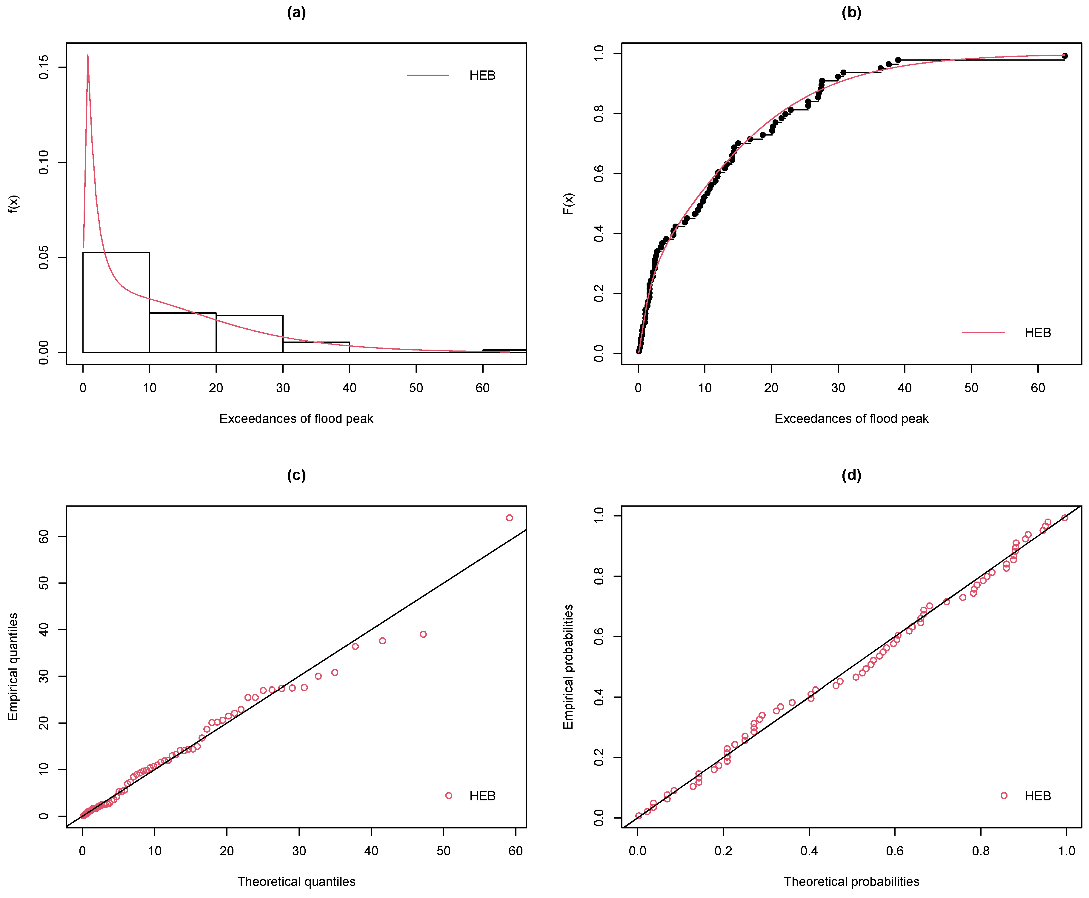
The fitted pdf and cdf plots, the quantile-quantile (Q-Q) plot, and the probability-probability (P-P) plots of the HEB model for the Wheaton river data are given in Figure 4. The points in the Q-Q and P-P plots are almost in a straight line. We can infer that the HEB model yields the best fit for the Wheaton river data.

6.3. Kiama Blowhole Data

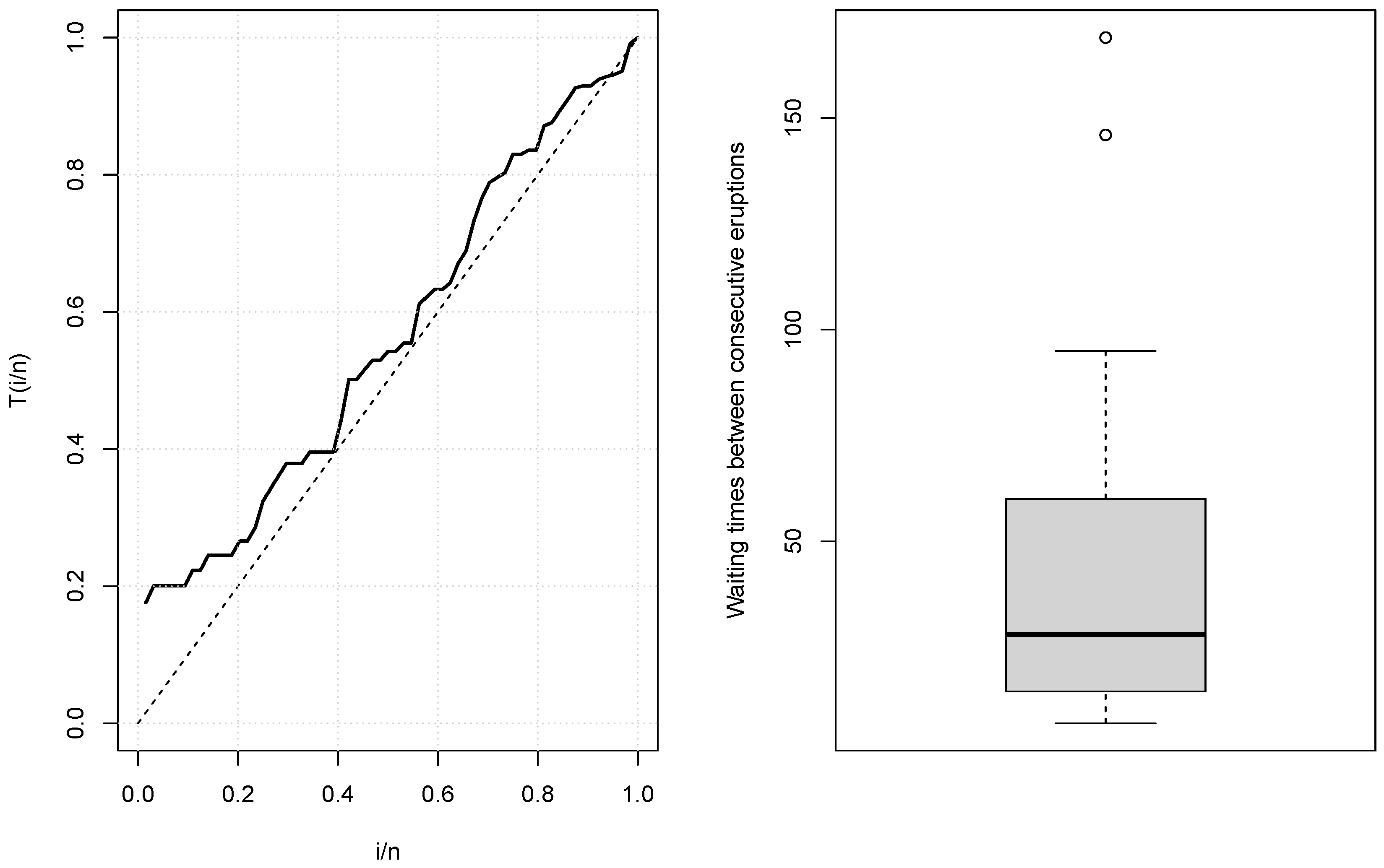
Here, the considered data set is the waiting times between consecutive eruptions of the Kiama Blowhole used in [12] to fit the HEE distribution. Figure 5 displays the TTT plot and box plot for the data, and we can see that the observations are right-skewed and with an increasing hrf that is applicable under the HEB model.

Table 3. ML estimates, SEs (in parentheses), and goodness-of-fit-measures of the models for the Kiama Blowhole data.

Distribution	Estimates			KS	p Value	AD	CM	ASAE
HEB	61.601	0.362	2.406	0.085	0.741	0.583	0.063	0.021
($\lambda ,\theta ,\delta$)	(12.2480)	(0.1770)	(1.5820)
HEL	0.038	0.395	2.091	0.091	0.670	0.631	0.068	0.021
($\lambda ,\theta ,\delta$)	(0.0080)	(0.1940)	(1.5420)
HEE	0.030	146,785.300	58.237	0.103	0.507	0.852	0.114	0.025
($\lambda ,\theta ,\delta$)	(0.0040)	(8398.7530)	(9.7700)
MOB	71.973	0.348		0.099	0.553	0.772	0.103	0.026
($\lambda ,\theta$)	(23.2651)	(0.2374)
GB	1.064	49.364		0.147	0.126	1.583	0.239	0.042
($\theta ,\lambda$)	(0.0819)	(4.9325)
EE	1.731	28.579		0.123	0.291	0.962	0.143
($\alpha ,\beta$)	(0.3200)	(4.1710)						-
EL	0.859	0.045		0.127	0.252	1.046	0.159	0.030
($\alpha ,\beta$)	(0.1540)	(0.0060)
EW	0.351	0.586	32.630	0.095	0.607	0.861	0.120	0.029
($\alpha ,\sigma ,\theta$)	(0.2514)	(2.8828)	(93.8733)
MOE	0.035	2.067		0.121	0.302	0.962	0.113	0.025
($\lambda ,\theta$)	(0.0070)	(0.8340)
MOL	0.033	0.364		0.097	0.581	0.733	0.094	0.025
($\lambda ,\theta$)	(0.0103)	(0.2413)
PL	0.909	0.070		0.115	0.361	0.889	0.126	0.028
($\lambda ,\theta$)	(0.0751)	(0.0209)

lists the ML estimates with SEs and goodness-of-fit-measures for different models. We can see that the HEB model has the minimum KS statistic with a large p value, and the AD, CM, and ASAE statistics have the smallest values. We can conclude that the HEB model performs well among the considered competitive models.

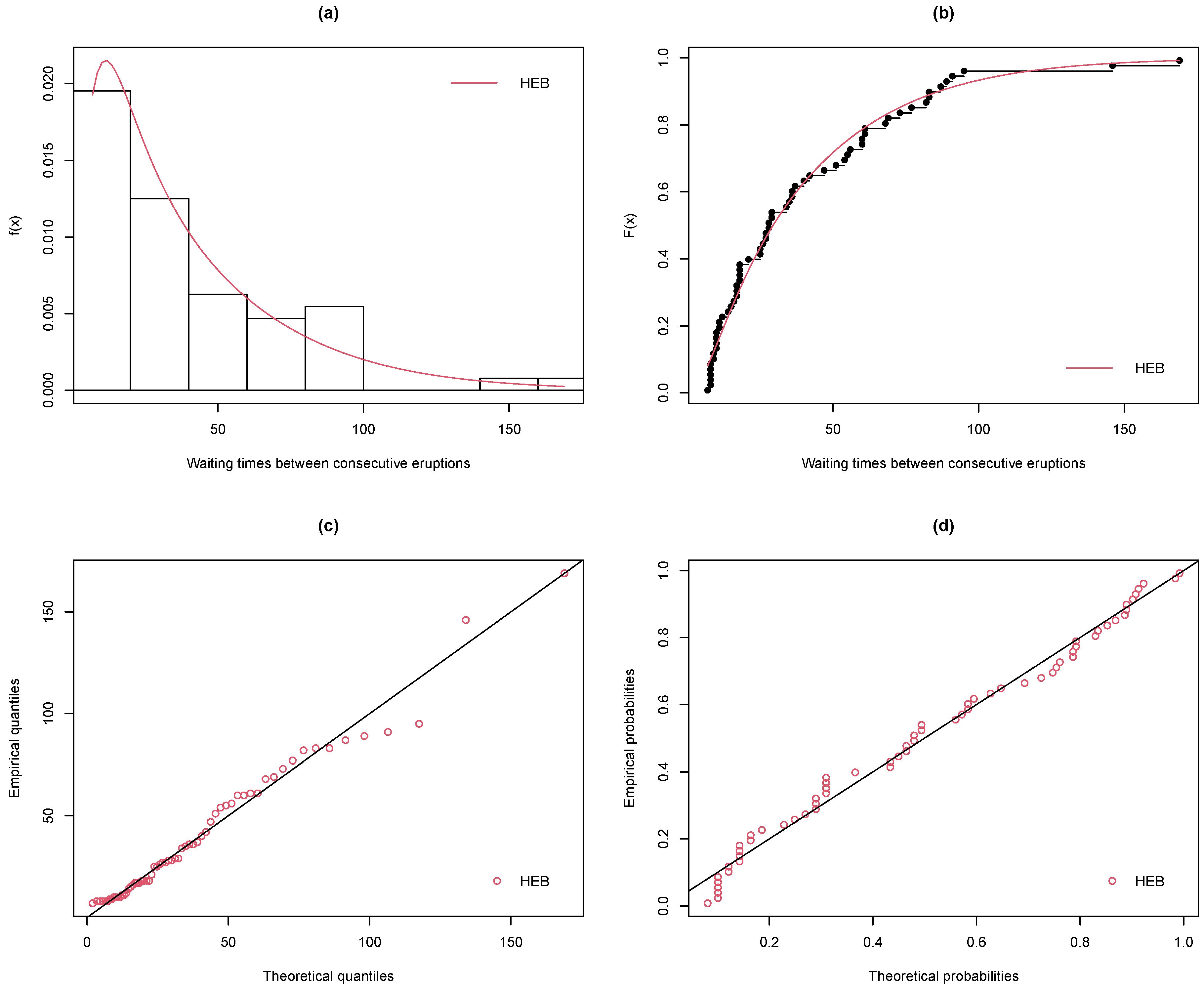
The fitted pdf and cdf plots, the Q-Q plot, and the P-P plot of the HEB model for the Kiama Blowhole data are displayed in Figure 6. The points in the Q-Q and P-P plots are almost in a straight line. We can infer that the HEB model yields the best fit for the Kiama Blowhole data.

7. Sampling Plan

7.1. Method

Here, we look forward to introducing an ASP based on the assumption that the lifetimes of sample products follow the HEB distribution. The number of items to be examined and the maximum possible number of defects in them for acceptance are the major concerns of an ASP. The number of defects when the test is terminated at a predetermined time is recorded. We accept the lot with a probability of at least $p^{*}$ if the number of defects out of n inspected items does not exceed the maximum possible number of defects (c) at time t. When the number of defects exceeds c before the specified time t, the lot is rejected. Thus, the minimum sample size required for the decision rule is the primary interest of our study.

Assume that the lifetime distribution follows the HEB distribution, with known $\theta$ and $\delta$ and unknown $\lambda$, so that the average lifetime is solely dependent on $\lambda$. We recall that the cdf of the HEB distribution is given by

$$G(t;\lambda ,\theta ,\delta )=1-\frac{{\theta }^{\frac{1}{\delta }}\left(3e^{-\frac{2t}{\lambda }}-2e^{-\frac{3t}{\lambda }}\right)}{{\left(1-\overline{\theta }{\left[3e^{-\frac{2t}{\lambda }}-2e^{-\frac{3t}{\lambda }}\right]}^{\delta }\right)}^{\frac{1}{\delta }}},t>0.$$

Let ${\lambda }_0$ be the required minimum average lifetime. Then, the following equivalence holds:

$$G(t;\lambda ,\theta ,\delta )\le G(t;{\lambda }_0,\theta ,\delta )\iff \lambda \ge {\lambda }_0.$$

The ASP is characterized by the following elements:

• The number of units n on the test;
• The acceptance number c;
• The maximum test duration t;
• The ratio $\frac{t}{{\lambda }_0}$, where ${\lambda }_0$ is the specified average lifetime and t is the maximum test duration.

For the sake of consumers, the lot with a true average life $\lambda$ less than ${\lambda }_0$ should be rejected by the ASP. As a result, the consumer’s risk should not exceed the value $1-p^{*}$, where $p^{*}$ is a lower bound for the probability that a lot is rejected by the ASP. The triplet $\left(n,c,\frac{t}{{\lambda }_0}\right)$ characterizes the ASP for a given $p^{*}$. We can obtain the acceptance probability by using a binomial distribution for sufficiently large lots. The main goal is to find the smallest sample size n for known c and $\frac{t}{{\lambda }_0}$ values so that

$$L\left(p_0\right)=\sum _{i=0}^c\left(\genfrac{}{}{0pt}{}{n}{i}\right)p_0^i{(1-p_0)}^{n-i}\le 1-p^{*},$$

where $p_0=G(t;{\lambda }_0,\theta ,\delta )$ is the failure probability before time t.

Table 4. Minimum sample size for specified $p^{*},\frac{t}{{\lambda }_0},\lambda =1.3,\theta =2,\mathrm{and}\delta =2.5$ for the binomial approximation.

${\mathit{p}}^{*}$	c	$\frac{\mathit{t}}{{\mathit{\lambda }}_0}$
		0.68	0.84	0.99	1.1	1.3	1.42	1.62	1.81	2	2.5
	0	4	3	2	2	2	1	1	1	1	1
	1	7	5	4	4	3	3	3	2	2	2
	2	11	8	6	6	5	4	4	4	3	3
	3	14	11	8	7	6	6	5	5	5	4
	4	18	13	10	9	8	7	6	6	6	5
0.75	5	21	15	12	11	9	9	8	7	7	6
	6	24	18	14	13	11	10	9	8	8	7
	7	27	20	16	14	12	11	10	10	9	8
	8	31	23	18	16	14	13	11	11	10	9
	9	34	25	20	18	15	14	13	12	11	11
	10	37	27	22	20	17	15	14	13	12	12
	0	8	5	4	4	3	3	2	2	2	1
	1	12	9	7	6	5	4	4	3	3	3
	2	17	12	9	8	7	6	5	5	4	4
	3	21	15	12	10	8	7	7	6	6	5
	4	24	18	14	12	10	9	8	7	7	6
0.95	5	28	20	16	14	12	11	9	9	8	7
	6	32	23	18	16	13	12	11	10	9	8
	7	36	26	21	18	15	14	12	11	10	9
	8	39	29	23	20	16	15	13	12	11	10
	9	43	31	25	22	18	16	15	13	13	11
	10	46	34	27	24	20	18	16	15	14	12

displays the minimum values of n for $p^{*}=0.75,0.95$, $\frac{t}{{\lambda }_0}=0.68,0.84,0.99,1.1,1.3,1.42,1.62,1.81,2,2.5$, $c=0,1,2,\dots ,10$, $\lambda =1.3$, $\theta =2$, and $\delta =1.5$.

For large values of n and small values of $p_0$, we can use the Poisson approximation with parameter $\alpha =n{p}_0$ as

$$L_1\left(p_0\right)=\sum _{i=0}^c\frac{{\alpha }^i}{i!}{e}^{-\alpha }\le 1-p^{*}.$$

(6)

The minimum values of n satisfying (6) are obtained in the same way as above, and are given in

Table 5. Minimum sample size for specified $p^{*},\frac{t}{{\lambda }_0},\lambda =1.3,\theta =2,\mathrm{and}\delta =2.5$ for the Poisson approximation.

${\mathit{p}}^{*}$	c	$\frac{\mathit{t}}{{\mathit{\lambda }}_0}$
		0.68	0.84	0.99	1.1	1.3	1.42	1.62	1.81	2	2.5
	0	5	4	3	3	2	2	2	2	2	2
	1	8	6	5	5	4	4	4	4	3	3
	2	12	9	8	7	6	6	5	5	5	5
	3	15	12	10	9	8	7	7	6	6	6
	4	19	14	12	11	9	9	8	8	7	7
0.75	5	22	17	14	12	11	10	9	9	9	8
	6	26	19	16	14	12	12	11	10	10	9
	7	29	22	18	16	14	13	12	11	11	10
	8	32	24	20	18	15	14	13	13	12	12
	9	35	27	22	20	17	16	15	14	13	13
	10	39	29	24	21	18	17	16	15	15	14
	0	9	7	6	5	5	4	4	4	4	4
	1	14	11	9	8	7	7	6	6	6	5
	2	19	14	12	11	9	9	8	8	7	7
	3	23	18	14	13	11	11	10	9	9	8
	4	27	21	17	15	13	12	11	11	10	10
0.95	5	31	24	19	17	15	14	13	12	12	11
	6	35	26	22	20	17	16	15	14	13	13
	7	39	29	24	22	19	17	16	15	15	14
	8	43	32	26	24	20	19	18	17	16	15
	9	46	35	29	26	22	21	19	18	18	17
	10	50	38	31	28	24	22	21	20	19	18

.

The operating characteristic (OC) function of the ASP $\left(n,c,\frac{t}{\lambda }\right)$ gives the probability of accepting the lot. It is given by

$$L\left(p\right)=\sum _{i=0}^c\left(\genfrac{}{}{0pt}{}{n}{i}\right)p^i{(1-p)}^{n-i},$$

where $p=G(t;\lambda ,\theta ,\delta )$. The OC function acts as a base for the choices of n and c for given values of $p^{*}$ and $\frac{t}{{\lambda }_0}$. By considering the fact that

$$\frac{t}{\lambda }=\frac{t/{\lambda }_0}{\lambda /{\lambda }_0},$$

the OC values for the ASP $\left(n,c,\frac{t}{\lambda }\right)$ are obtained and displayed in

Table 6. The OC values for the ASP $\left(n,c,\frac{t}{\lambda }\right)$.

${\mathit{p}}^{*}$	n	c	$\frac{\mathit{t}}{{\mathit{\lambda }}_0}$	$\frac{\mathit{\lambda }}{{\mathit{\lambda }}_0}$
				2	4	6	8	10	12
0.75	11	2	0.68	0.87663	0.99462	0.99935	0.99987	0.99996	0.99999
	8	2	0.84	0.87247	0.99424	0.99929	0.99985	0.99996	0.99998
	6	2	0.99	0.88618	0.99493	0.99937	0.99986	0.99996	0.99999
	6	2	1.1	0.83142	0.99150	0.99890	0.99976	0.99993	0.99997
	5	2	1.3	0.80897	0.98982	0.99865	0.99970	0.99991	0.99997
	4	2	1.42	0.86029	0.99319	0.99911	0.99980	0.99994	0.99998
	4	2	1.62	0.77858	0.98724	0.99825	0.99960	0.99988	0.99996
	4	2	1.81	0.68743	0.97867	0.99694	0.99929	0.99978	0.99992
	3	2	2	0.82267	0.99005	0.99863	0.99969	0.99990	0.99996
	3	2	2.5	0.65521	0.97233	0.99586	0.99902	0.99969	0.99988
0.95	12	2	0.68	0.84890	0.99300	0.99914	0.99982	0.99995	0.99998
	9	2	0.84	0.83090	0.99168	0.99895	0.99978	0.99993	0.99998
	8	2	0.99	0.77053	0.98717	0.99831	0.99963	0.99989	0.99996
	7	2	1.1	0.75753	0.98601	0.99813	0.99959	0.99988	0.99996
	6	2	1.3	0.70575	0.98124	0.99740	0.99941	0.99982	0.99993
	6	2	1.42	0.61972	0.97191	0.99594	0.99907	0.99971	0.99989
	5	2	1.62	0.62109	0.97173	0.99588	0.99905	0.99971	0.99989
	5	2	1.81	0.49991	0.95393	0.99289	0.99831	0.99947	0.99980
	5	2	2	0.38527	0.92982	0.98851	0.99719	0.99911	0.99966
	5	2	2.5	0.16147	0.83365	0.96790	0.99156	0.99719	0.99889

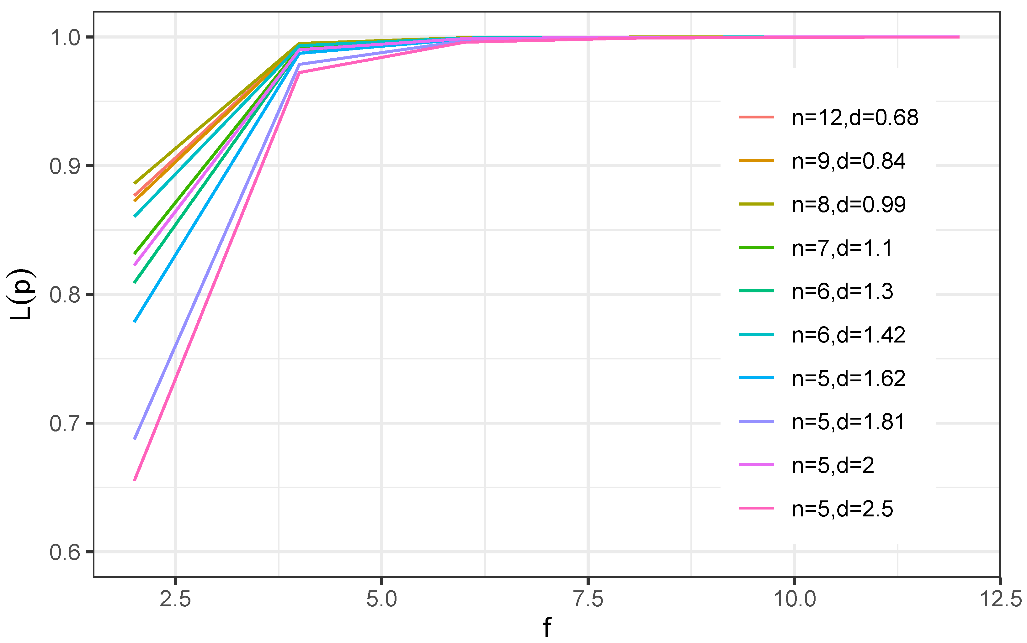
. Figure 7 shows the OC curve for $p^{*}=0.75$, $d=\frac{t}{{\lambda }_0}$, and $f=\frac{\lambda }{{\lambda }_0}$.

For the sake of producers, the lot with $\lambda$ greater than ${\lambda }_0$ should be accepted. The probability of rejecting a lot when $\lambda$ is greater than ${\lambda }_0$, called producer’s risk, can be found by determining $p=G(t;\lambda ,\theta ,\delta )$ and with the help of a binomial distribution. For a specified producer’s risk of, say 0.05, it would be interesting to know what value of $\frac{\lambda }{{\lambda }_0}$ will ensure that a producer’s risk is less than or equal to 0.05 if the proposed ASP is adopted. The smallest value of $\frac{\lambda }{{\lambda }_0}$ must satisfy the following inequality:

$$\sum _{i=0}^c\left(\genfrac{}{}{0pt}{}{n}{i}\right)p_0^i{(1-p_0)}^{n-i}\ge 0.95.$$

(7)

For the given ASP $\left(n,c,\frac{t}{\lambda }\right)$ and prefixed $p^{*}$,

Table 7. Minimum values of $\frac{\lambda }{{\lambda }_0}$ required for acceptability of a lot with producer’s risk of 0.05 for the ASP $\left(n,c,\frac{t}{\lambda }\right)$, $\lambda =1.3,\theta =2,\mathrm{and}\delta =1.5$.

${\mathit{p}}^{*}$	c	$\frac{\mathit{t}}{{\mathit{\lambda }}_0}$
		0.68	0.84	0.99	1.1	1.3	1.42	1.62	1.81	2	2.5
	0	6.51	6.89	6.53	7.25	8.57	6.41	7.31	8.16	9.02	11.27
	1	3.03	3.05	3.11	3.46	3.36	3.67	4.19	3.43	3.79	4.74
	2	2.44	2.47	2.4	2.66	2.76	2.54	2.89	3.23	2.73	3.41
	3	2.09	2.2	2.09	2.1	2.2	2.4	2.34	2.61	2.89	2.84
	4	1.96	1.95	1.91	1.96	2.11	2.06	2.03	2.27	2.51	2.51
0.75	5	1.81	1.79	1.8	1.87	1.88	2.05	2.1	2.05	2.26	2.3
	6	1.72	1.75	1.72	1.81	1.86	1.87	1.93	1.89	2.08	2.14
	7	1.64	1.66	1.66	1.66	1.72	1.73	1.79	2	1.95	2.02
	8	1.62	1.64	1.61	1.63	1.72	1.76	1.69	1.89	1.85	1.93
	9	1.57	1.57	1.57	1.61	1.63	1.67	1.76	1.8	1.76	2.2
	10	1.53	1.52	1.54	1.59	1.64	1.59	1.68	1.72	1.69	2.12
	0	9.39	9.05	9.47	10.53	10.67	11.65	10.68	11.93	13.18	11.27
	1	4.15	4.34	4.41	4.46	4.71	4.46	5.09	4.68	5.17	6.46
	2	3.17	3.18	3.14	3.23	3.49	3.44	3.44	3.84	3.57	4.46
	3	2.68	2.69	2.75	2.71	2.74	2.71	3.09	3.06	3.38	3.61
	4	2.34	2.42	2.42	2.42	2.51	2.53	2.63	2.63	2.9	3.13
0.95	5	2.17	2.17	2.21	2.23	2.36	2.41	2.34	2.61	2.59	2.82
	6	2.06	2.06	2.06	2.11	2.13	2.19	2.32	2.38	2.38	2.6
	7	1.97	1.98	2.02	2.01	2.07	2.14	2.14	2.21	2.21	2.44
	8	1.88	1.91	1.93	1.94	1.93	2	2.01	2.07	2.09	2.31
	9	1.83	1.82	1.85	1.88	1.9	1.88	2.03	1.97	2.17	2.2
	10	1.76	1.79	1.8	1.83	1.88	1.88	1.93	2.02	2.07	2.12

displays the minimum values of $\frac{\lambda }{{\lambda }_0}$ required to satisfy (7).

7.2. Illustration

Allow the lifetime to follow the HEB distribution with parameters $\lambda =1.3,\theta =2,\mathrm{and}\delta =1.5$. Suppose that our interest is an ASP with an unknown average lifetime of 1000 h, such that the termination time is 1100 h. The consumer’s risk is prefixed at $1-p^{*}=0.25$. The required number of n is 6 for an acceptance number of $c=2$ and $\frac{t}{{\lambda }_0}=1.1$, according to Table 4. Hence, the considered ASP is $\left(n=7,c=2,\frac{t}{{\lambda }_0}=1.1\right)$. During the test time, we have a confidence level of 0.75 that the average lifetime is at least 1000 h if at most two failures out of six are observed. The ASP under consideration for the Poisson approximation is $\left(n=7,c=2,\frac{t}{{\lambda }_0}=1.1\right)$. From Table 6, the OC values of the ASP $\left(n=6,c=2,\frac{t}{{\lambda }_0}=1.1\right)$ under the binomial case with a consumer’s risk of 0.25 are: $0.83142,0.99150,0.99890,0.99976,0.99993,0.99997$ for $\frac{\lambda }{{\lambda }_0}=2,4,6,8,10,12$, respectively.

As a result, if $\frac{\lambda }{{\lambda }_0}=2$, the producer’s risk is 0.17. The producer’s risk is negligible if it is 10 or 12. From Table 7, the minimum value of $\frac{\lambda }{{\lambda }_0}$ giving a producer’s risk of 0.05 is 3.23. Thus, if the consumer’s risk is fixed at a specified level, then the quality can be reached by a predetermined ratio.

7.3. Application

Here, we consider a data set regarding software reliability obtained from a software development project, which was presented in [18] and which worked out the ASP in [19,20,21]. The 13 ordered failure times are:

$$519,968,1430,1893,2490,3058,3625,4422,5218,5823,6539,7083,7487.$$

Let the testing time be 3600 h and the prefixed average lifetime be 3000 h. The ASP is adopted under the assumption that the lifetime follows the HEB distribution. The Q-Q plot and goodness-of-fit statistics guarantee a good agreement ($\theta =1.758011\times {10}^{13}$, $\delta =4.921590\times {10}^2$). By taking $\frac{t}{{\lambda }_0}=1.2$, $p^{*}=0.95$, and $n=13$, we obtain c as 6. Thus, the considered ASP is ($n=13,c=6,\frac{t}{{\lambda }_0}=1.2$). We accept the lot if and only if the number of failures is at most 6. There are six values here that are less than t. Thus, we accept the lot.

8. Conclusions

The Harris extended Bilal (HEB) distribution is a three-parameter extension of the Bilal distribution that we suggested. It is obtained by applying the Harris extended scheme to the Bilal distribution. The aim of the two additional shape parameters is to provide more flexibility to the Bilal distribution. The Bilal distribution is included as a sub-distribution, and the HEB distribution can be considered as a generalization of the Marshall–Olkin Bilal distribution. The corresponding pdf is unimodal and better suited for right-skewed data sets. The hrf can increase, or have an upside-down bathtub shape, or a roller coaster shape. The mathematical properties were discussed and are meant for comparative purposes with respect to the members of the Harris extended family. Then, an emphasis on the statistical HEB model’s efficiency was made. The performance of the model parameter estimation was evaluated using a simulation study. The proposed HEB model provided a better modeling of hydrological data when compared to the competing models. We developed an acceptance sampling plan that has a lifetime following the HEB distribution. The operating characteristic values, the minimum sample size that corresponds to the maximum possible defects, and the minimum ratios of lifetime associated with the producer’s risk were discussed. The results were illustrated using a real data set. The perspectives of this work are numerous, including the applications to various applied fields (biology, medicine, engineering, informatics, etc.); the extension to the multidimensional case with use in regression and classification modeling; and the discrete version for the modeling of count data.

References

- Abd-Elrahman, A.M. Utilizing ordered statistics in lifetime distributions production: A new lifetime distribution and applications. J. Probab. Stat. Sci. 2013, 11, 153–164. [Google Scholar]
- Abd-Elrahman, A.M. A new two-parameter lifetime distribution with decreasing, increasing or upside-down bathtub-shaped failure rate. Commun. Stat.-Theory Methods 2017, 46, 8865–8880. [Google Scholar] [CrossRef]
- Maya, R.; Irshad, M.; Arun, S. Application of U–statistics in Estimation of Scale Parameter of Bilal Distribution. Philipp. Stat. 2021, 70, 67–82. [Google Scholar]
- Altun, E.; El-Morshedy, M.; Eliwa, M. A new regression model for bounded response variable: An alternative to the beta and unit-Lindley regression models. PLoS ONE 2021, 16, e0245627. [Google Scholar] [CrossRef] [PubMed]
- Altun, E. A new one-parameter discrete distribution with associated regression and integer-valued autoregressive models. Math. Slovaca 2020, 70, 979–994. [Google Scholar] [CrossRef]
- Maya, R.; Irshad, M.; Arun, S. Farlie- Gumbel- Morgenstern Bivariate Bilal Distribution and Its Inferential Aspects Using Concomitants of Order Statistics. J. Prob. Stat. Sci. 2021, 19, 1–20. [Google Scholar]
- Akhter, Z.; Almetwally, E.M.; Chesneau, C. On the Generalized Bilal Distribution: Some Properties and Estimation under Ranked Set Sampling. Axioms 2022, 11, 173. [Google Scholar] [CrossRef]
- Aly, E.E.A.; Benkherouf, L. A new family of distributions based on probability generating functions. Sankhya B 2011, 73, 70–80. [Google Scholar] [CrossRef]
- Harris, T.E. Branching processes. Ann. Math. Stat. 1948, 19, 474–494. [Google Scholar] [CrossRef]
- Marshall, A.W.; Olkin, I. A new method for adding a parameter to a family of distributions with application to the exponential and Weibull families. Biometrika 1997, 84, 641–652. [Google Scholar] [CrossRef]
- Cordeiro, G.M.; Mansoor, M.; Provost, S.B. The Harris extended Lindley distribution for modeling hydrological data. Chil. J. Stat. 2019, 10, 77–94. [Google Scholar]
- Pinho, L.G.B.; Cordeiro, G.M.; Nobre, J.S. The Harris extended exponential distribution. Commun. Stat. Theory Methods 2015, 44, 3486–3502. [Google Scholar] [CrossRef]
- Gupta, R.D.; Kundu, D. Theory and methods: Generalized exponential distributions. Aust. N. Z. J. Stat. 1999, 41, 173–188. [Google Scholar] [CrossRef]
- Mudholkar, G.S.; Srivastava, D.K. Exponentiated Weibull family for analyzing bathtub failure-rate data. IEEE Trans. Reliab. 1993, 42, 299–302. [Google Scholar] [CrossRef]
- Ghitany, M.; Al-Mutairi, D.K.; Balakrishnan, N.; Al-Enezi, L. Power Lindley distribution and associated inference. Comput. Stat. Data Anal. 2013, 64, 20–33. [Google Scholar] [CrossRef]
- Nadarajah, S.; Bakouch, H.S.; Tahmasbi, R. A generalized Lindley distribution. Sankhya B 2011, 73, 331–359. [Google Scholar] [CrossRef]
- Castillo, E.; Hadi, A.S.; Balakrishnan, N.; Sarabia, J.M. Extreme Value and Related Models with Applications in Engineering and Science; Wiley: Hoboken, NJ, USA, 2005. [Google Scholar]
- Wood, A. Predicting software reliability. Computer 1996, 29, 69–77. [Google Scholar] [CrossRef]
- Jose, K.; Tomy, L.; Thomas, S.P. On a Generalization of the Weibull Distribution and Its Application in Quality Control. Stochastics Qual. Control. 2018, 33, 113–124. [Google Scholar] [CrossRef]
- Lio, Y.; Tsai, T.R.; Wu, S.J. Acceptance sampling plans from truncated life tests based on the Burr type XII percentiles. J. Chin. Inst. Ind. Eng. 2010, 27, 270–280. [Google Scholar] [CrossRef]
- Tomy, L.; Jose, M. Applications of HLMOL-X Family of Distributions to Time Series, Acceptance Sampling and Stress-strength Parameter. Austrian J. Stat. 2022, 51, 124–143. [Google Scholar] [CrossRef]
Figure 1.
Plots of the pdf of the HEB distribution.
Figure 2.
Plots of the hrf of the HEB distribution.
Figure 3.
TTT plot (left) and box plot (right) based on the Wheaton river data.
Figure 4.
The fitted pdf (a), cdf (b), Q-Q plot (c), and P-P plot (d) of the HEB model for the Wheaton river data.
Figure 5.
TTT plot (left) and box plot (right) for the Kiama Blowhole data.
Figure 6.
The fitted pdf (a), cdf (b), Q-Q plot (c), and P-P plot (d) of the HEB model for the Kiama Blowhole data.
Figure 7.
The OC curve of the ASP .