

Τhe “GPS/GNSS on Boat” Technique for the Determination of the Sea Surface Topography and Geoid: A Critical Review

1
School of Science and Technology, Hellenic Open University, 18 Par. Aristotelous Str., 26335 Patras, Greece
2
Department of Civil Engineering, University of Peloponnese, 1 M. Alexandrou Str., Koukouli, 26334 Patras, Greece
*
Author to whom correspondence should be addressed.
Coasts 2022, 2(4), 323-340; https://doi.org/10.3390/coasts2040016
Submission received: 30 September 2022
/
Revised: 3 November 2022
/
Accepted: 7 November 2022
/
Published: 12 December 2022
(This article belongs to the Topic Drones for Coastal and Coral Reef Environments)
Abstract
:The opening up of the global positioning system (GPS) for non-military uses provided a new impetus for the study of the sea surface topography (SST) and geoid, especially in coastal areas which are important from the viewpoint of the climate crisis. The application of the “GPS/GNSS on boat” method, as an alternative to traditional (indirect and direct) methods, has provided detailed SST maps in coastal and oceanic areas with an accuracy of up to few centimeters. In this work we present the first critical review concerning the evolution of the “GPS/GNSS on boat” method over a period of 27 years. Twenty-one papers, covering the 27 years of related research, are critically reviewed, focusing on the innovations they introduce, the solutions they present and the accuracy they achieve. Further improvement of the method, principally of its accuracy, and the extension of SST measurements to additional coastal environments open new perspectives for the examination of open geophysical problems and climate change.
1. Introduction
In the present article we critically review the evolution of the “GPS/GNSS on boat” method, used for determining the sea surface topography (SST) and geoid, through the scientific publications that supported each contribution [1,2,3,4,5,6,7,8,9,10,11,12,13,14,15,16,17,18,19,20,21]. GPS and GNSS symbolize the so-called “global positioning system” and “global navigation satellite system”, respectively. The second is wider and involves the first one and other relevant systems which use satellites for determining the position of an object. The precise determination of sea surface heights (SSHs) and geoid in open seas and in coastal areas is one of the problems that attracts modern research interest. This is due to several factors. For example, climate change affects the height and the whole shape of the SST. Moreover, the shape of the geoid and the SST are of special interest in continental shelf areas, closed seas and sea bays [22]. Finally, precise knowledge of the SST can reveal interesting geological structures on the seabed.
Determining the SST has traditionally been achieved by either indirect or direct techniques. The indirect techniques involve astro-geodetic measurements of vertical deflection (VD) [23,24,25,26], measurements of heights using tide gauges [27,28] and gravity measurements [29,30,31,32,33,34]. Using these measurements, the SST or the geoid is calculated through mathematical models.
The direct techniques involve measurements from altimetry satellites (TOPEX/POSEIDON, Jason-1, etc.) [35,36,37,38,39,40,41,42,43,44,45] and the “laser scanner on plane” technique [46,47,48,49]. However, both indirect and direct techniques have weaknesses.
Applying the indirect methods to determine the SST and the geoid, the accuracy achieved is very low, including errors of the order of a few meters. The direct methods, on the other hand, although they directly measure the SST, suffer from double errors, as the position of the satellite or the position of the laser scanner is determined by a GPS/GNSS system in cooperation with an inertial system. Thus, the error of determining the position of the satellite or the plane is added to the inevitable error of the altimeter measurements. In particular, direct techniques face serious difficulties in coastal areas or enclosed seas, where the shape of the earth’s geomorphology creates visual obstacles. In addition, the application of direct techniques is highly expensive.
The “GPS/GNSS on boat” method attempts to overcome the problems of both indirect and direct techniques. Its main advantage is that it can perform direct measurements of SST without the aforementioned double errors, as it contains only the error of the GNSS receiver. Thus, it can be used to correct the SST calculations based on the satellite altimetry and tide gauge. Additionally, the “GPS/GNSS on boat” technique can focus on coastal areas or closed seas, detecting small anomalies and details of the sea surface. GPS/GNSS data can be processed by applying the method of precise point positioning (PPP) or the kinematic differential GPS/GNSS (D-GPS/GNSS) method in cooperation with GPS/GNSS stations on land. Figure 1 shows a schematic representation of the “GPS/GNSS on boat” technique.
2. Critical Review of the Papers Dealing with the Application of the “GPS/GNSS on Boat” Technique Which Illustrate the Evolution of the Method
Table 1 shows, in chronological order, the published scientific works concerning the application of the “GPS/GNSS on boat” technique for determining the SST and geoid. This critical chronological review of the articles offers the possibility to present the evolution of the method through the innovations introduced in each work. The table includes information about the area/location of the measurements, the sea GPS/GNSS platform, the methodology used for processing the GPS/GNSS data, the number of GPS/GNSS used and the accuracy achieved.
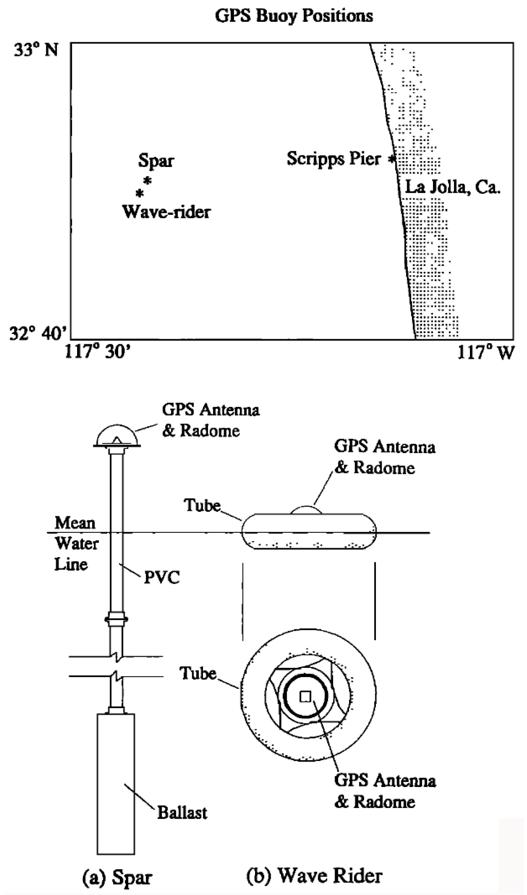
In their pioneering work, Kelecy et al. (1994) [1] used GPS for the first time for determining sea surface heights. For this purpose, they placed a GPS receiver on two different types of floating buoys (wave rider and spar design) in order to investigate whether dynamic effects related to the platform affect the accuracy of the measurements. The measurements were resolved by two fixed receivers located on the roof of the Institute of Geophysics and Planetary Physics (Scripps Institute of Oceanography) at a distance of 1.2 and 15 km from the GPS buoy positions. The measurements were carried out on two separate days for 45 min each day. Tidal noise was removed from the time series. The results were compared with marine topography measurements provided by the EIS 1 satellite altimeter. The orbit of the satellite during the two-day period of the measurements (21 and 29 November 1991) passed over the point where the two buoys were placed. The small difference in height estimation (just 6 cm) provided by the method with respect to earlier satellite estimates, showed for the first time that the use of the “GPS on boat” technique is an easy, cheap and reliable method to determine the sea surface. Figure 2 shows the location of the measurements and a schematic representation of the two buoy design.
The second application of a buoy with a GPS receiver was presented four years later in the work of Key et al. (1998) [2]. A GPS receiver was deployed at 16 sites along the California coast, 10 km from Texaco’s Harvest platform. A simple wave rider buoy equipped with a GPS receiver was used to estimate sea surface heights (SSHs). The results from the GPS measurements were compared with the altimetry measurements of the TOPEX/POSEIDON satellite, which measured above the buoy area during the experiments. Very small differences of a few centimeters were observed between the marine topography heights provided by the GPS buoy and the TOPEX satellite altimeter measurements. Moreover, the differences between the former estimations with the corresponding ones of the National Oceanic and Atmospheric Administration (NOAA) were also very small (1.5–2 cm). This agreement indicated for the second time that the use of floating GPS can be a reliable alternative method of measuring SSHs.
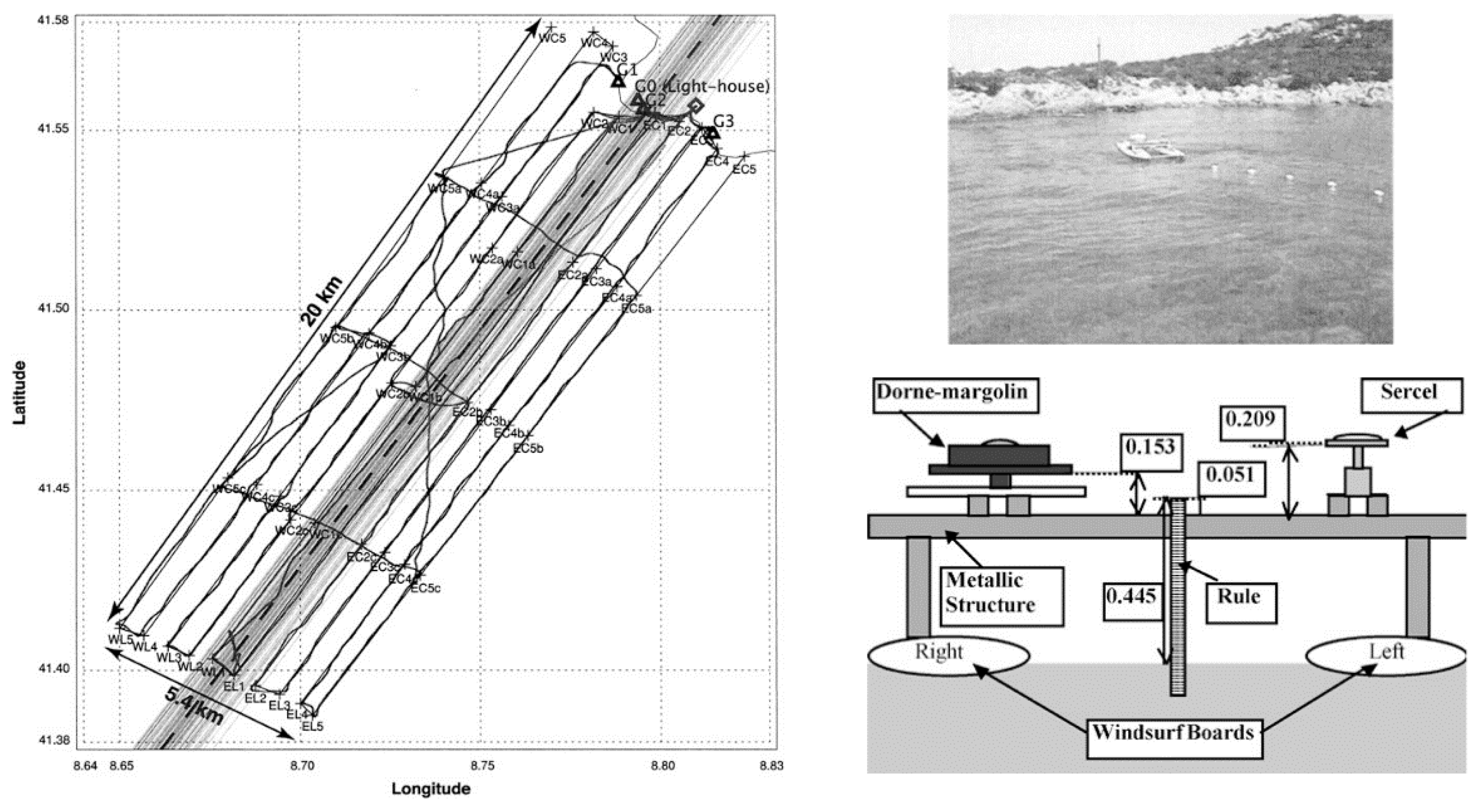
Important progress in the evolution of the “GPS/GNSS on boat” technique was achieved in 2003 thanks to the work of Bonnefond et al., performed in coastal areas of Corsica (2003) [3]. The purpose of this work was not only to record the local SSHs and calibrate the measurements using TOPEX/Poseidon and Jason-1 satellites results, but also to determine the local marine geoid slope. In this view, two efforts described in [3] have been done. The first one took place in 1998 [3] using GPS buoys and showed that it was very difficult to cover large areas simply using GPS buoys. Thus, in the following year they conducted a new experiment placing for the first time two GPS receivers on a catamaran-type floating platform. Figure 3 (Right) shows this facility.
This innovative, for that period, platform enabled coverage of an area of 20.0 × 5.4 km (Figure 3, Left). The analysis of the data was based on two static GNSS receivers on land whereas the GeoGenius software was used applying the D-GPS/GNSS) method. Data from GPS was filtered using a Vondrak filter with a period of 120 s. Comparing the results taken from the two GPS receivers and the measurements of tide gauges revealed insignificant differences, with standard deviations from 1.9 to 2.7 cm. Taking all parameters into account, the final SST estimated accuracy was about 2 cm.
Rocken et al. (2005) [4] presented their work on the floating GPS technique that was applied for the first time in the open sea (Caribbean Sea). Two experiments were carried out (in 2002 and 2003) with a GPS receiver mounted on a 138,000 ton ship. A second GPS receiver was also mounted for confirmation. Moreover, the PPP method was used for the first time for processing the experimental data. This method proved to be ideal for applications in open seas, far from land [50]. After removing the tide, the authors determined the SSHs and the geoid over the ship’s path. Comparing their results with the local CARIB97 geoid they found a 32 cm mean difference between them. In Figure 4 these differences are pointed out. Taking into account the scatter and noise of the data, the authors estimate the accuracy of their determination of the SST in the order of 10 cm.
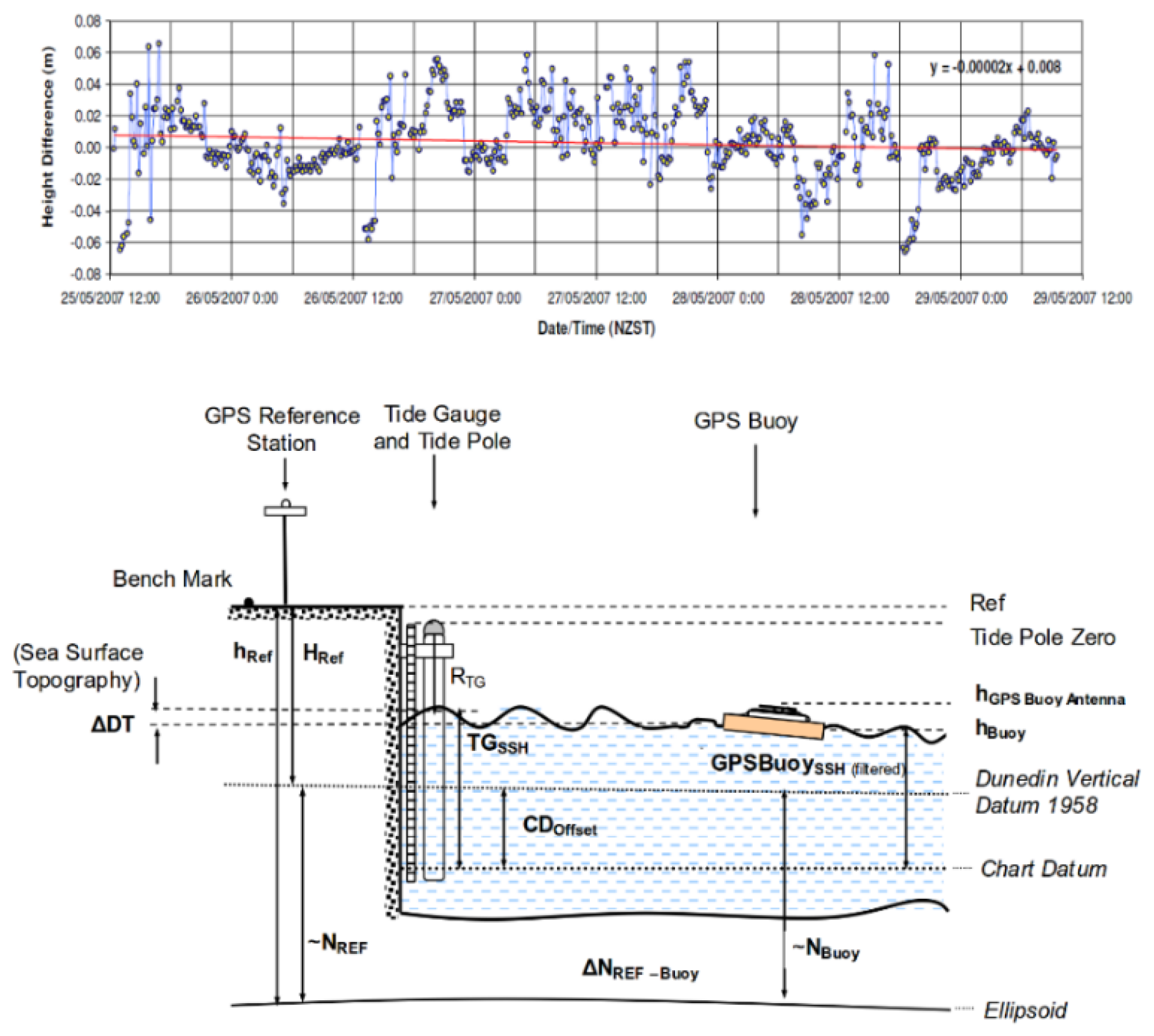
Marshall & Denys (2009) [5] attempted to estimate the accuracy of the GPS buoy method in the determination of sea heights. For this reason, two GPS buoys were placed in close proximity to existing tide gauges at Chalmers harbor and Dunedin pier in New Zealand. The GPS data collection period was four days. The aim of the work was to find out the difference in height estimates obtained from the GPS buoys and tide gauges in order to estimate the accuracy of the former. The difference in precision and mean difference in height between the tide gauges and buoys was estimated to be less than 1 mm (as an average value), while the standard deviation was estimated to be ±2 cm. This indicated that the GPS buoy technique works well with a high level of accuracy and thus it is suitable for determining sea heights (Figure 5).
The next contribution concerning the evolution of the “GPS/GNSS on boat” method concerns the work of Foster et al. (2009) [6]. With this work, the method was applied on a research ship for the first time. The authors noted that changes in the ship’s inclination and movement due to the waves caused serious difficulties in obtaining accurate results. Thus, they proposed a complex methodology based on the simultaneous use of GPS and a radar water level gauge installed onboard the ship. (Figure 6). This was the first time that a second measuring instrument had been implemented on a ship. The joint use of the aforementioned apparatus on a research ship allowed the successful determination of the SST at a distance of 200 km from the coast. The ship used in this mission was equipped with a Trimble NetRS single-frequency GPS receiver (Westminster, CO, USA) recording at a sampling rate of 1 Hz and a VEGAPULS62 radar scanner (Schiltach, Germany), recording at the same frequency. The GPS data were analyzed using the TRACK module of the GAMIT program [51]. To remove the effect of tides and the medium-term climate effects, they used a five-minute moving average filter. The distance of the ship (in port) from the GPS reference station (on land), through which the kinematic differential solution was performed, was approximately 25 km, while that from the nearest tide gauge, through which the ocean tide was subtracted, was approximately 2.5 km. However, despite this small initial distance, the ship moved distances of up to 200 km from the reference stations and this resulted in greater uncertainty in the estimation of SSHs. The initial estimate of the standard deviation of the SSHs, in the unfiltered data, reached 69 cm but after moving average filtering, it dropped to 13.3–16.1 cm. The relatively high uncertainties of the SSH estimations were due to both the high ocean tide and the multipath effect as well as to the use of a single-frequency GPS receiver. Nevertheless, even if this work did not provide a reliable map of the SST, the innovation of adding a radar water level gauge contributed significantly to the further development of the “GPS on boat” method.
The paper published by Bouin et al. (2009) [7] concerns the shipboard GPS SST mapping in the sea around Santo Island, Vanuatu. This work brought together the results from three research campaigns in 2004, 2006 and 2007, and provided a detailed local map of the SST with an accuracy of 5–15 cm. A GPS with a sampling frequency of 1 Hz was used and an area up to 80 km from the coast was covered. The GPS data were processed using the GAMIT 10.32 software, while for the application of the D-GPS/GNSS method they exploited a free network of permanent GPS ground stations, including nearby stations (Santo, Port Vila, and Noumea).
While processing the data, the researchers noticed that the height of the GPS antenna on the ship changed depending on the speed of the ship. Thus, they proposed, for the first time, a methodology to overcome this difficulty. To link the position of the ship’s GPS antenna to the surface of the water they used a second GPS mounted on a specially designed buoy (Figure 7).
Lycourghiotis and Stiros (2010) [8] applied the “GPS on-boat” method in a large coastal area in the Gulf of Patras and the southern Ionian Sea (Greece). Measurements took place between June and July 2008 on a 43 ft long sailing boat using a Topcon HipperPro type GPS receiver. Throughout the experiment, weather data was systematically collected, such as intensity and wind direction, atmospheric pressure, temperature and moisture and the slope of the boat. GPS data was analyzed using Pinnacle software, while four land GPS stations were used, for the application of the D-GPS/GNSS method, located at the University of Patras, the Village Valmi, Lefkada and Kefalonia. Using a three-step methodology, three types of noise were removed from the SSHs data: (a) outliers, (b) systematic offsets with amplitude of 10 cm and (c) random noise using a moving average filter. Taking into account all the types of uncertainty, it was estimated that the SSHs error was smaller than 15 cm. Moreover, in this work, for the first time, the presentation of an SST map with contour lines for the study area was attempted.
The work of Reinking et al. (2012) [9] is the next major contribution to the “GNSS on boat” methodology. This introduced the following innovations: (a) the use of GNSS methodology, i.e., the utilization of satellites beyond those of the GPS system, (b) the use of PPP methodology for the analysis of GNSS data and (c) the use, apart from the main ship, of an escort vessel with a GNSS receiver. The goal of this work was to determine the effect of the dynamic movement of the ship on the GNSS data. The field work was carried out with the help of a cruise ship named AID-Ablu on 19 and 20 March 2011, operating the route between Tenerife and Madeira, in the open Atlantic Ocean. Thus, the data were collected from one route. The researchers installed Trimble 4700 GNSS receivers on the 252 m long vessel. The ship was sailing at a maximum speed of 40 knots. Another receiver, a Trimble 4700, was mounted on the escort ship, which followed the ship at a distance of 0.5 nM. All receivers recorded at a frequency of 1 Hz. The long distance of the base stations from the ship’s course led them to adopt the PPP methodology for the kinematic resolution of the GNSS data. Tide subtraction was performed using data from tide gauges. Noise removal was performed using a moving average filter (see Figure 8). Finally, the authors estimated that the accuracy achieved in calculating SST was about 5 cm.
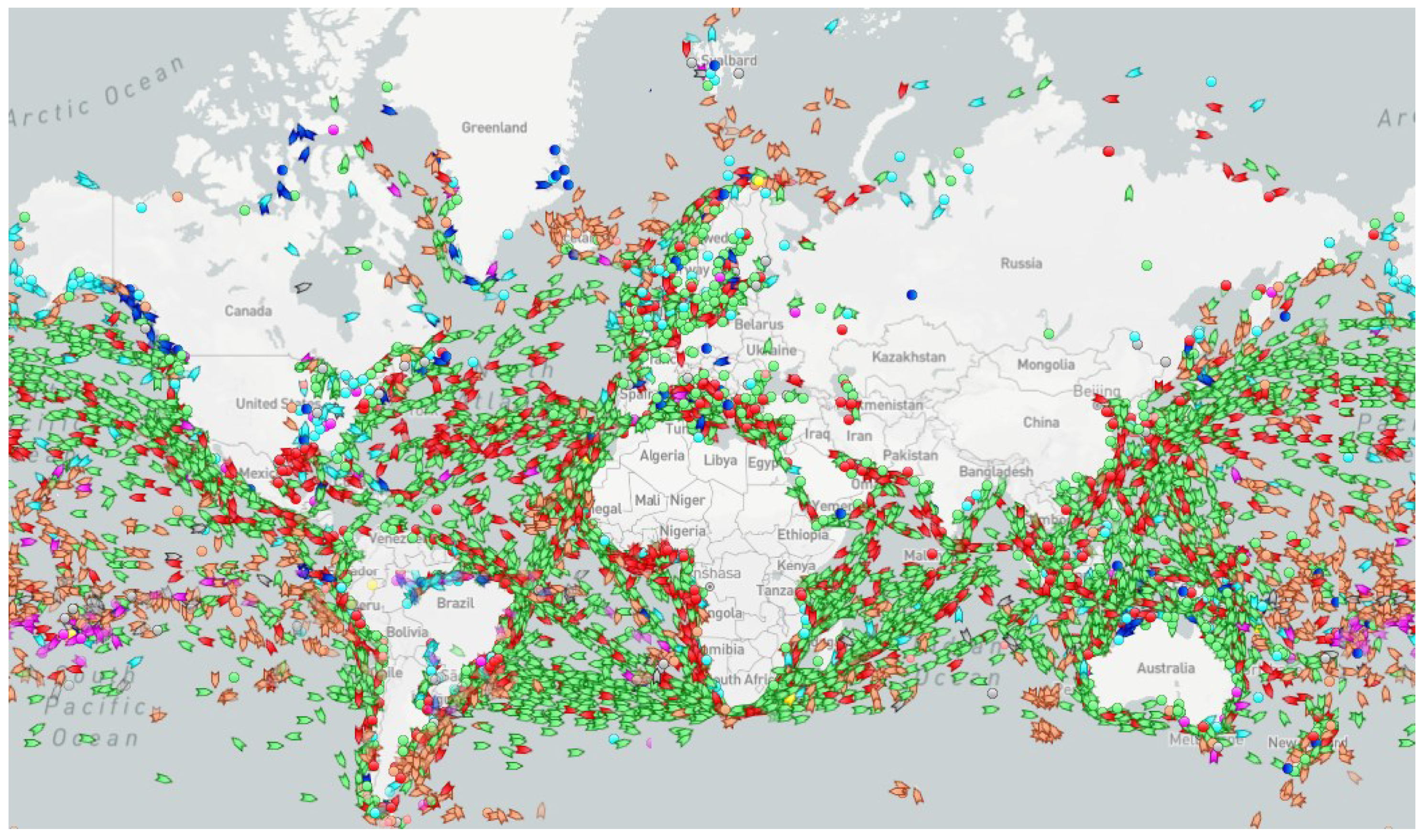
The work proposed the use of the “GPS/GNSS on boat” technique in the determination of SST through the utilization of ships performing oceanic routes around the planet (see Figure 8). This could have important applications as ship routes cover a large part of the ocean surface, whereas due to their repeated routes the accuracy of the results could be significantly improved. The latter idea would be fully utilized a few years later [21].
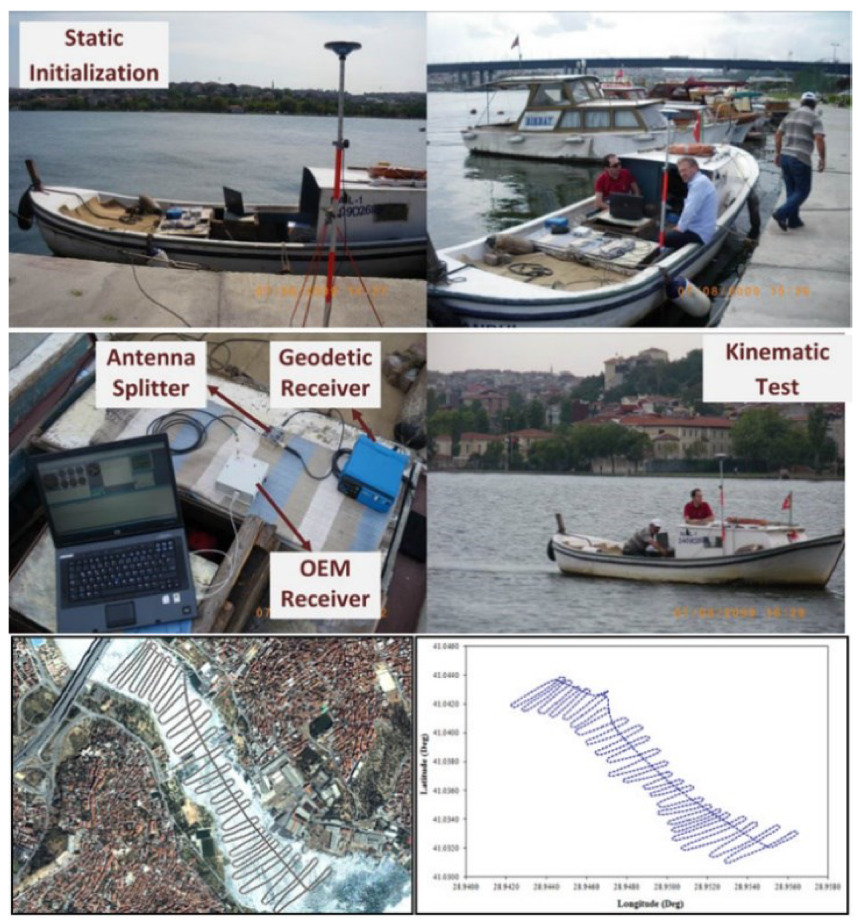
Ocalan and Alkan (2012, 2013) [10,11] attempted to investigate the limits of the PPP technique in the context of the “GPS on boat” method, comparing their results obtained using PPP with the corresponding ones using the D-GPS/GNSS method. It was the first time that both methods had been used comparatively. It was also the first time that the “GPS on boat” method had been applied in a closed bay. In fact, they took measurements over a two-hour period in Halic (Golden Horn) of Istanbul (Turkey) using an Ashtech Z-Xtreme GNSS receiver (Mumbai, India) mounted on a small boat (Figure 9). It was found that the web service solutions of the PPP method were consistent with the results of the kinematic differential method. Thus, it was proved at a certain level of certainty that PPP can be used successfully in the context of the “GPS on boat” method.
Guo et al. (2014) [12] estimated, for the first time, the SSHs following a complex procedure which involved the joint use of a GNSS on a boat and a ship-borne gravimeter. The ship gravimeter and the GNSS measured anomalies in gravity and SSHs along the ship’s track, respectively. The new method was applied on the coastal sea of the Shandong Peninsula in China. Deflections of the vertical (DOVs) on the ship were estimated from the measured gravities using the least squares co-location method. This work provided an original method connecting the height anomaly difference with DOVs, gravity and geodetic data. The precision of the DOV along the ship track was better than 1, whereas the precision of ship-borne SSHs was better than 5 cm and those of the SSHs differences better than 3.5 cm.
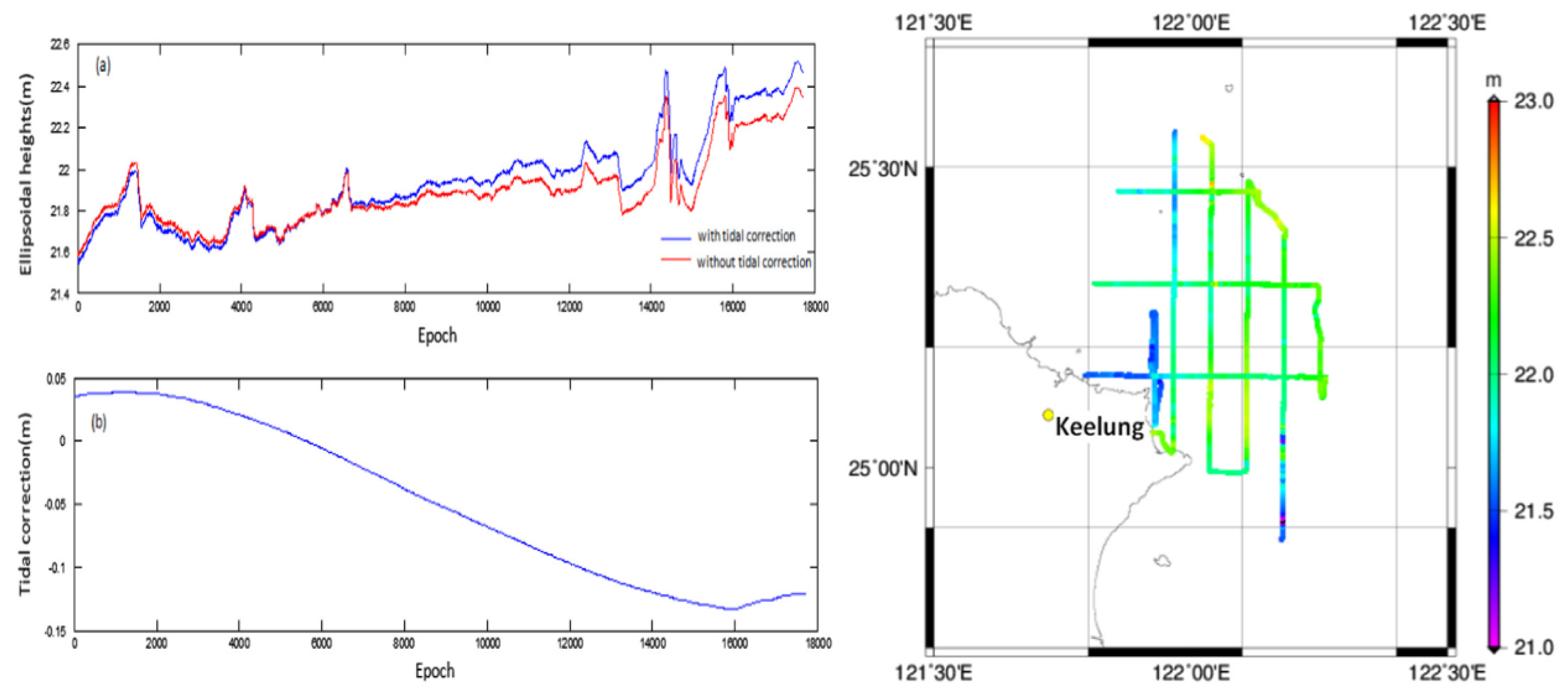
The next paper we consider was published by Guo et al. (2016) [13] and presented the first application of the ship-borne GNSS method improved with the crossover point adjustment technique. The study area was the coastal sea near Keelung, located on the north exit of the Taiwan Strait, east of the West Pacific Ocean. GNSS data was collected in 2007 on six voyages in total with a sampling rate of 1 Hz. The GNSS receiver used was a LEICA SR530 with antennae of AT502 Pillar. The GNSS onboard data was processed with the PPP method [52] and filtered by the Gaussian filter with the window of 120 s. The NAO.99b model [53] was used to remove the ocean tide (Figure 10, Left) [13]. In this study there were 15 crossover points. Crossover analysis was used to analyze the SSHs of the crossover points and determine the SSHs accuracy. The crossover adjustment was used to calculate biases and drifts and correct them. In Figure 10 (Right), we can see the SSHs along the tracks of the ship. The practical results indicate that the SSH accuracy of crossover points can be improved by 2–5 cm after the ocean tidal correction.
The next contribution comes from the work of Morales Maqueda et al. (2016) [14]. For the first time, the “GPS on boat” method was applied on a lake while the GPS receiver was installed in a wave glider (Figure 11, Left). The experiment took place on the famous Loch Ness lake (Scotland) under mild weather and the GPS “traveled” 32 km along the length of the lake for about 25 h (Figure 11, Left) The PPP method was applied for the calculation of the SSHs. The D-GPS/GNSS method was also applied for quality control using the static GPS reference stations at Fort Augustus and Inverness. The GPS receivers were logging at 1 Hz. Moving average filters of 3 and 900 seconds were used to remove noise from the data. The calculation of SSHs along the lake revealed a shape of SST with a slope of −0.03 m/km which was in very good agreement with the EGM2008 geoid. After removing the geoid heights from the GPS SSHs, the height anomalies revealed a cyclic variation of ~2.5 cm. It was notable that the calculated accuracy of the GPS SSHs was found to be around 5 cm.
Lycourghiotis (2017) [15] presented an outline of the progress of the “GNSS on boat” method in view of the results of four different experiments which took place in different places over several years. One or more innovations were employed in each experiment. These concerned: (a) The installation of a GNSS receiver on a sailing boat in the Ionian Sea [8]. (b) The installation of two GNSS receivers on a plastic boat in the Corinthian Gulf [16]. (c) The development of a catamaran platform with four GNSS receivers as escort ships in the Gulf of Patras [17]. (d) The installation of a GNSS receiver on a passenger ship for six months [23]. The step-by-step development of the method by using these innovations in different environments allowed, in effect, the improvement of the method’s accuracy.
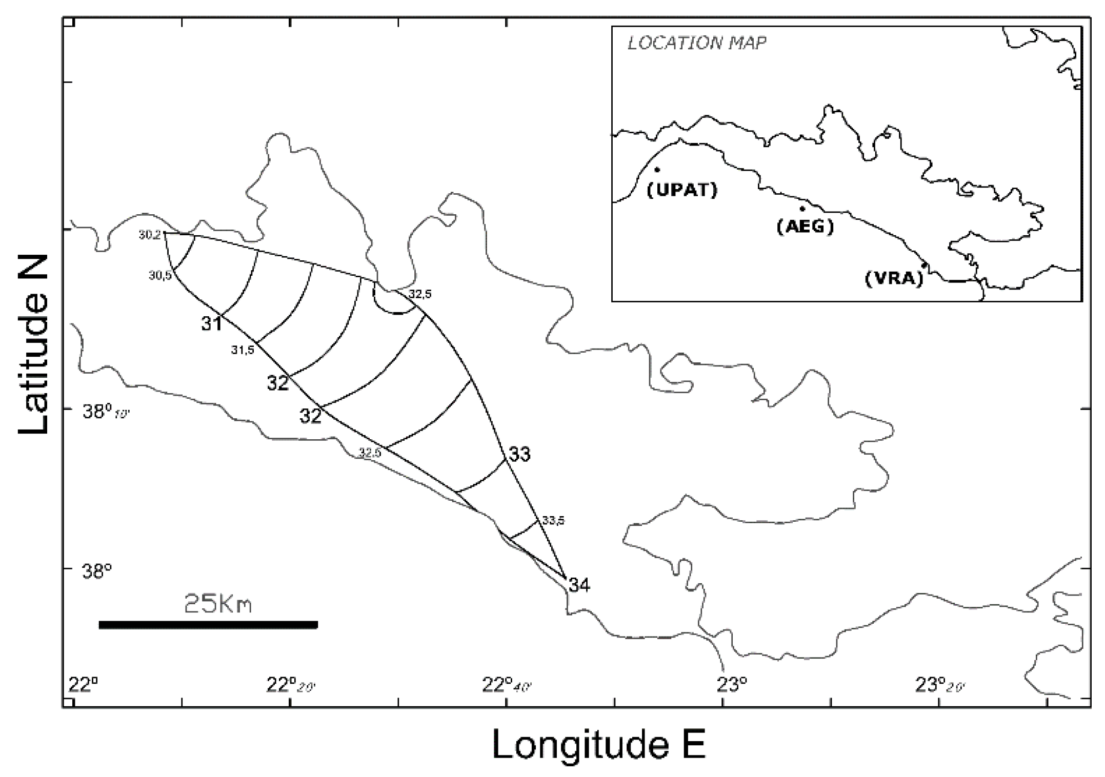
After the aforementioned first application of the “GNSS on boat” method in the Ionian Sea [8], the second application was made in the Corinthian Gulf (Greece) [16]. It was the first time that two GNSS receivers recording together had been used, in order to improve accuracy. Moreover, this area had been studied in the past with the “laser scanner on plane” method [46]. The study took place in the central-eastern part of the Gulf of Corinth and was conducted using a small boat carrying two GNSS receivers at a low altitude from the sea surface (1.1 m) to avoid excessive boat oscillations. Two Topcon HiperPro type GNSS receivers were mounted on a 16 ft long motorboat. Data analysis was based on a double-way path. The D-GPS/GNSS method was used in the first path and PPP in the second. Results from the two different methods were compared with each other and the results from the D-GNNS were confirmed by PPP. Τide effect was removed taking into account data from the “Posidonia” tide station. Using the “transmission of errors” formula the SSHs accuracy was found to be equal to 3.76 cm. Finally, an SST map of the study area was produced (Figure 12).
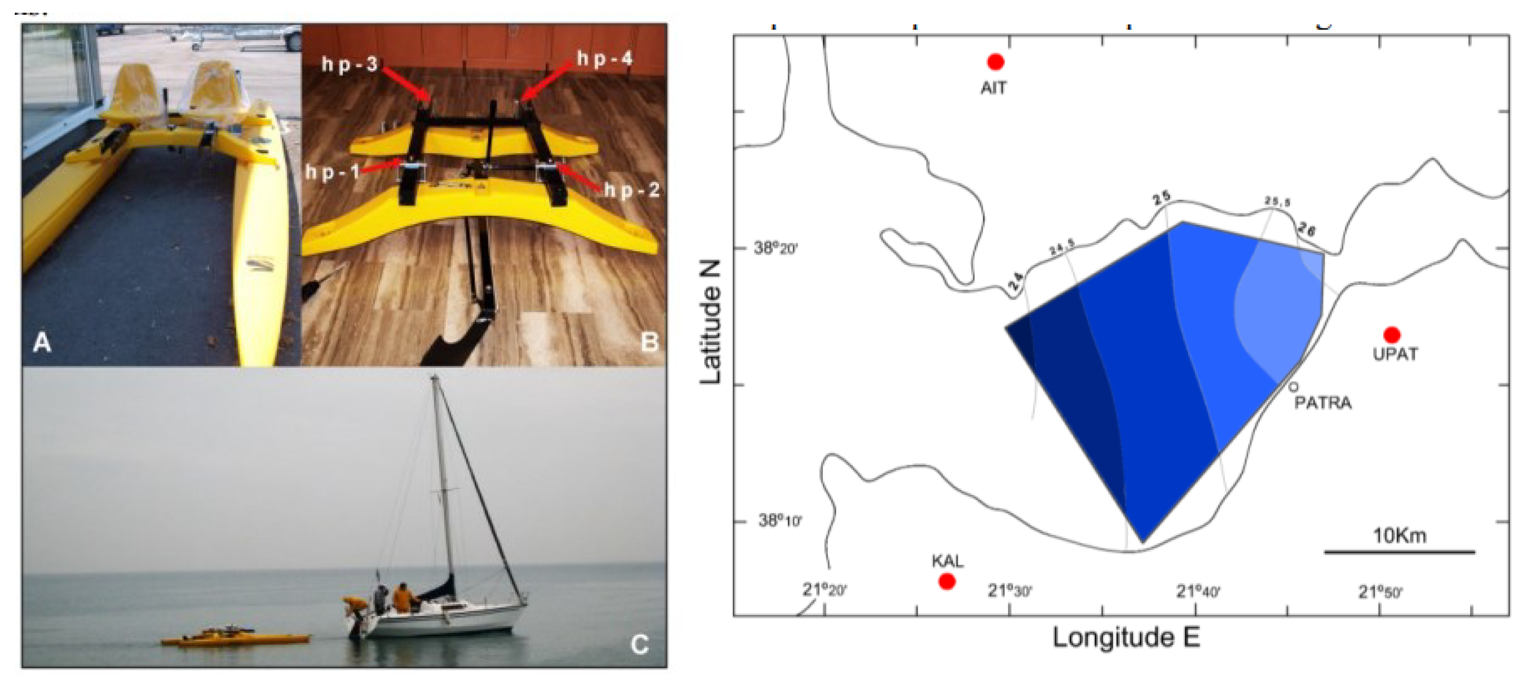
The next experiment towards further improving the accuracy of the “GPS/GNSS on boat” technique took place in the area of the Gulf of Patras [17]. Four GNSS receivers were placed on a catamaran platform. This special platform was designed to follow the ship at a distance of 15 m (Figure 13, Left). In this way, the effect of wave oscillation could be significantly reduced through digital correction of motion of the platform. Moreover, the multipath phenomenon was eliminated as the plastic material of the platform and the distance from the ship did not allow significant signal reflections. Four HiperPro GNSS receivers were placed a small distance from the sea surface (31–39 cm). GNSS sea measurements were subsequently analyzed in reference to three land receivers (Figure 13, Right). All receivers (rover and land) were recording at a frequency of 1 Hz. In a complex step-by-step analysis all sources of error were considered separately and using the formula of “transmission of errors” the accuracy calculated was equal to 5.43 cm. Finally, analysis led to the determination of the SST (mean sea level) of the study area (Figure 13, Right). Although four GPS system were used, the accuracy was worse than the previous application [16], and this seemed paradoxical. However, this accuracy could have been even lower (<3 cm) if an operational tide gauge had been in the area during the experiment. Unfortunately, the Patras tide gauge was out of order.
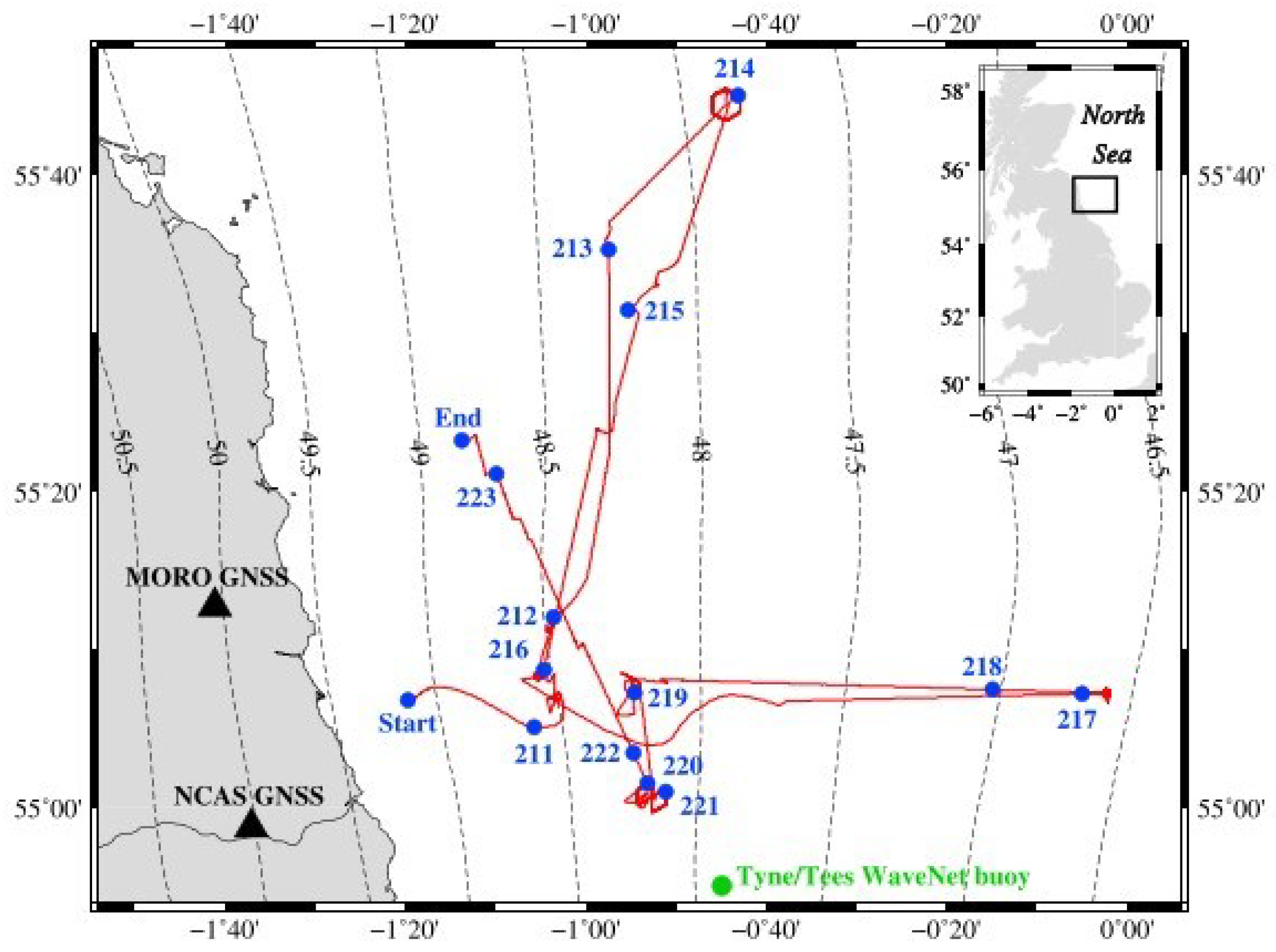
Continuing with our review analysis, an unmanned, self-propelled sea surface vehicle (wave glider) equipped with a GNSS receiver was used for the first time in the work of Penna et al. (2018) [18]. The new approach attempted to overcome limitations of common sea surface height instruments (tide gauges, satellite altimetry, and GNSS buoys). The implementation of the new method took place in the North Sea, on a thirteen-day trip, during which the unmanned vehicle traveled a 600 km track. Figure 14 illustrates the wave glider’s track. The SSHs measurements, performed under difficult weather conditions for a long time and long track, demonstrated the suitability of this approach. GNSS was recording at a frequency of 5 Hz. Tide effect was corrected using the finite element solution 2014b model and the geoid using the earth gravitational model 2008. For the analysis of the GNSS data the PPP method was used. The final estimate of the SSHs was made with a precision of 5–6 cm.
Recognizing the difficulties that exist especially in coastal areas, where the proximity to land and complex dynamics creates complications for the calculation of SSHs. Chupin et al. (2020) [19] presented two pioneering kinematic systems, based on GNSS, able to map the SSHs at the centimeter level: (1) A GNSS mounted on a floating carpet towed by a boat (named CalNaGeo); and (2) a combination of a GNSS antenna and an acoustic altimeter (named Cyclopée) mounted on an unmanned surface vehicle (USV). Figure 15 illustrates both systems.
To test both systems a number of field works were performed. To estimate the effect of speed on the water height measurements a first attempt was made, in the context of the so-called static mode, without horizontal movement, in the context of kinematic mode. GNSS was functioning at 1 Hz and the tests were carried out in two coastal zones in the Pertuis Charentais area (France) and in the Noumea lagoon (New Caledonia). After a systematic analysis of their data, the authors concluded that, although the ability of the CalNaGeo GNSS carpet and the Cyclopée systems to precisely measure SSH in motion had been demonstrated, there were yet uncertainties concerning the accuracy, both in terms of system biases and of GNSS processing.
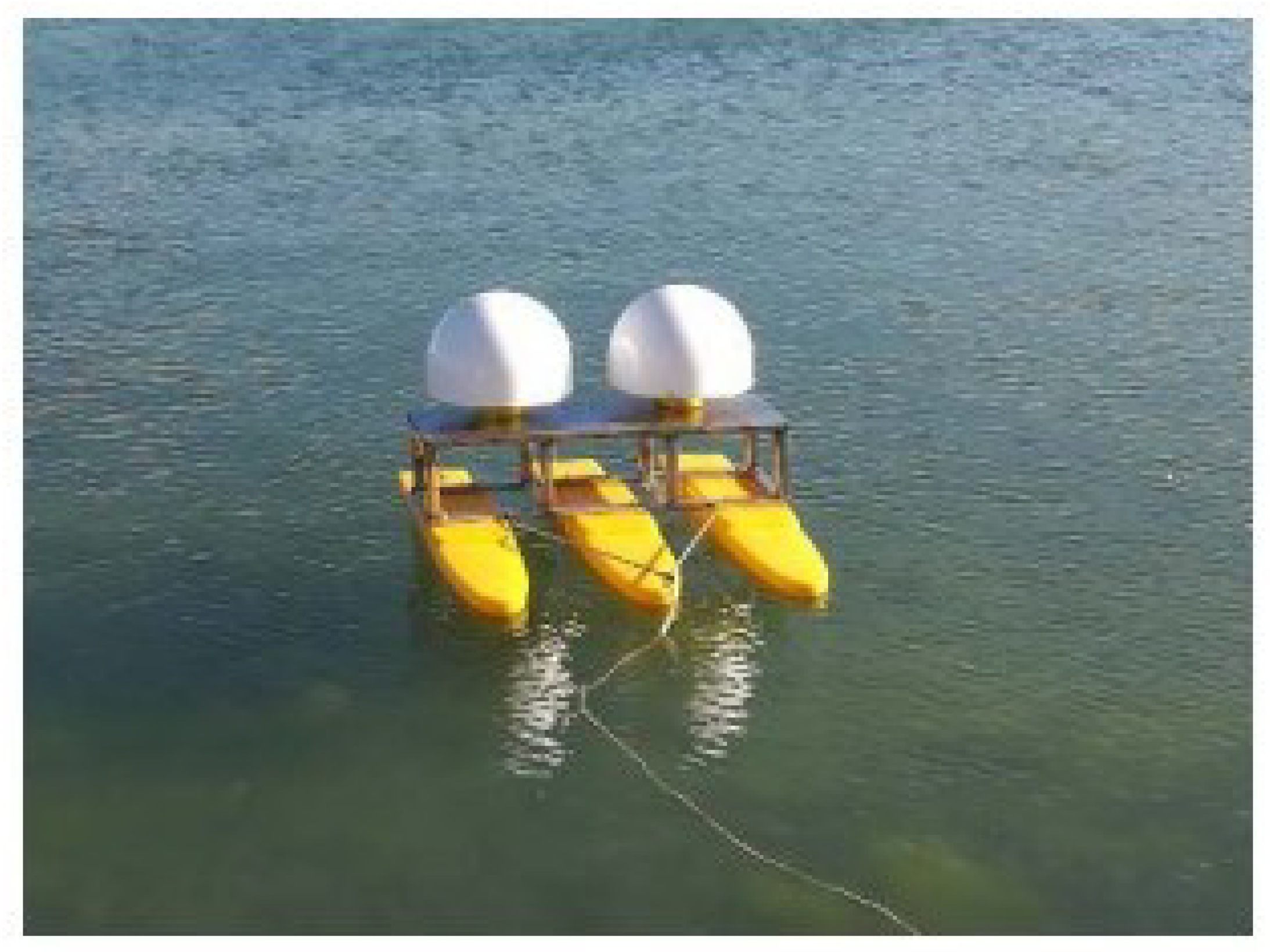
Wanlin et al. (2020) [20] conducted an experiment near Zhiwan Island (South China Sea) in order to determine the SSHs under the HY-2A altimetric satellite track. Two GPS mounted on a twined trimaran plastic platform was designed to measure the SSHs (Figure 16).
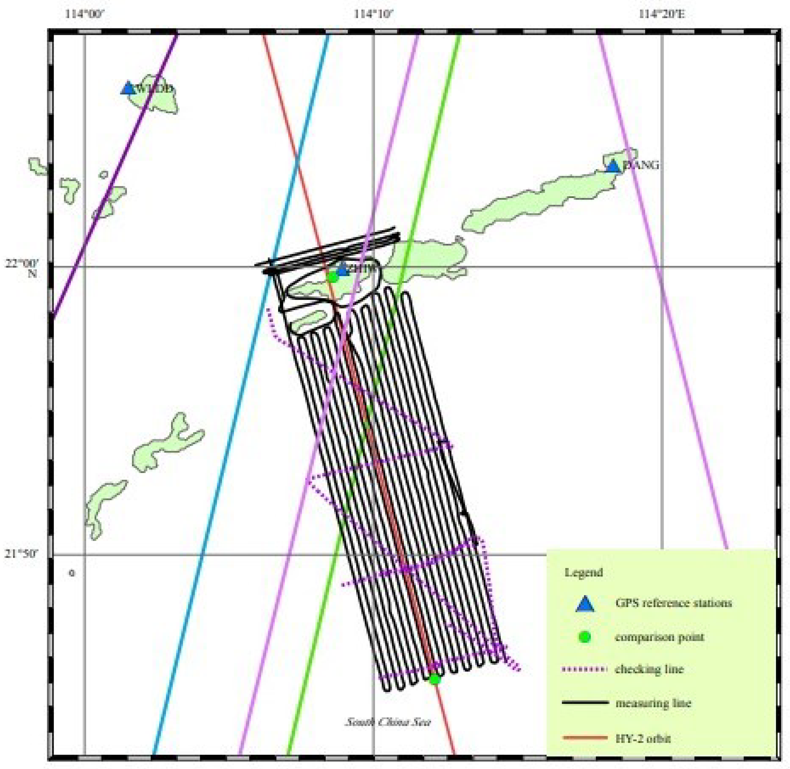
The experiment covered an area of 6 km × 28 km (Figure 17). GPS data were calculated with GAMIT software in the context of the D-GPS/GNSS method using three GPS reference stations on land. One tide gauge was also used in order to remove tide effect. The work provided an image of the SST in the experimental area with a surface slope of about 1.62 cm/km. Taking into account all parameters, such as tide gauge time-series, they calculated SSHs with an accuracy of 1.5–4.0 cm with a standard deviation of 0.2–2.4 cm.
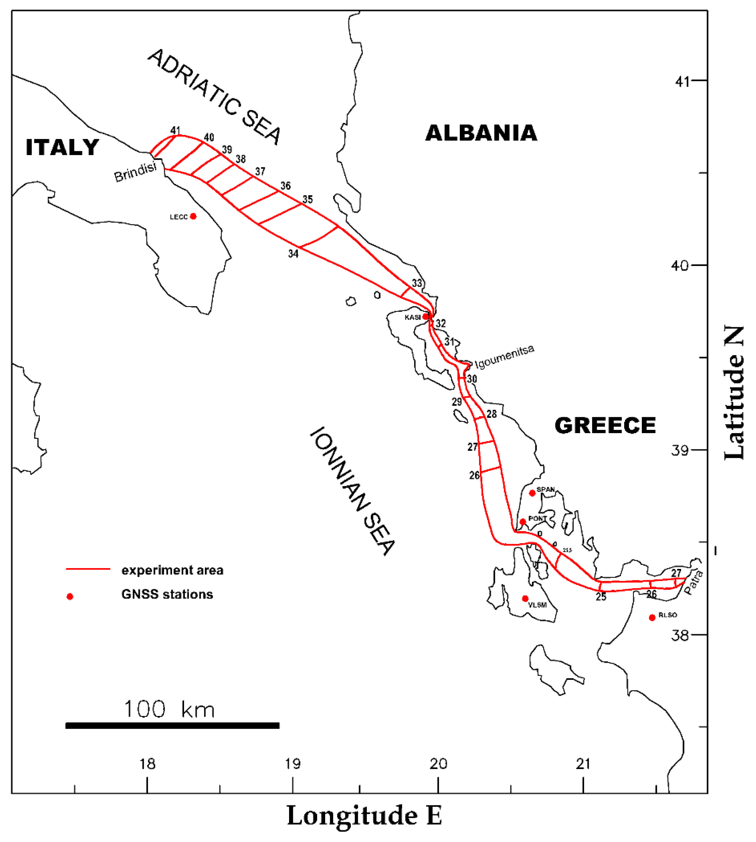
The work of Lycourghiotis (2021) [21] constitutes the most recent contribution concerning the methodology “GNSS on boat”. In this work GNSS measurements were performed for a period of six months utilizing the repeated route of a passenger ship between Patras (Greece) and Brindisi (Italy), exploiting for the first time the idea of gaining more accurate data by repeated measurements in the same area. The main pursuit was the improvement in accuracy of the SST estimation. The data, collected during the six-month period, was elaborated by adopting a double-path methodology and using the D-GPS/GNSS and PPP analysis jointly. A novel technique was developed and applied jointly with numerical filtering techniques and multi-parametric accuracy analysis to remove the meteorological tide factors. Figure 18 illustrates the SST map determined in the large area studied. A nearly constant slope of 4 cm/km in the N–S direction was determined. The SSHs determined were compared with the EGM96 geoid model with calculated differences between 0 and 48 cm. Finally, through a systematic analysis, the SST accuracy was estimated at about 3.31 cm.
3. Final Considerations
As already mentioned in the introduction, the aim of this critical review was to present the evolution of the “GPS/GNSS on boat” technique which has taken place in the last 27 years through the innovations introduced in the reviewed works. The presentation of these works allows us to formulate some critical considerations concerning the target/utility of the various innovations that have been introduced so far, with interest on the special features introduced by the “GPS/GNSS on boat” method, as well as the future development of the method and its various applications.
Starting with the innovations introduced in the past 27 years, we noted that they all faced different problems and thus contributed complementary to the overall development of the technique. The use of GPS on spar/wave rider buoys at the beginning of the “GPS/GNSS on boat” technique’s evolution offered a very simple and chip tool to demonstrate, for the first time, the validity of the technique to measure SSHs [1,2,3,5]. However, these devices allowed the measurement of SSHs only at specific points and therefore they could not lead to the determination of SST. Therefore, the replacement of GPS on spar/wave rider buoys by GPS/GNSS on moving vessels of various types and sizes for determining SST was an important step in the development of the technique [3,4,6,7,8,9,10,11,12,13,14,15,16,17,18,19,20,21]. In this context, various structures suitable for different marine environments were developed to overcome difficulties related to the particular characteristics of each study area. These involved the use of a single ship [3,4,6,8,10,11,12,13,14,16,18,20,21], the use of escort floating means [7,9,17,19] and the use of a self-propelled wave glider/unmanned surface vehicle [14,18]. A very important step was the application of the technique using cruise [9] or passenger ships [21]. The first successful efforts in this area opened the way for exploiting the huge number of voyages of these ships to determine the SST in different regions of the world. In this context, the use of the repeated routes of a particular ship was shown to increase the accuracy of SST determination [21].
The introduction of the GNSS methodology, i.e., the utilization of satellites in addition to those of the GPS system [9,12,13,15,16,17,18,19,21] and the joint use of more than one GPS or GNSS receivers [3,5,15,17,20] on the main ship/escort floating meant that as well as the joint use of a GPS/GNSS with another apparatus (radar water level gauge [6], gravimeter [12], acoustic altimeter [19]) constituted important contributions in the development of the “GPS/GNSS on boat” technique, principally in view of achieving greater accuracy. An important step in the development of the “GPS/GNSS on boat” technique was the application of the PPP procedure for processing the experimental data which proved to work successfully without GPS/GNSS stations on land. Thus, it proved to be ideal for application in open seas. Moreover, the joint use of the PPP and D-GPS/GNSS procedures in closed seas [10,14,15,16,17,19,21] increased the validity of the “GPS/GNSS on boat” technique.
Summarizing the discussion on the innovations presented above, the following suggestions should be considered, in order to achieve high accuracy in SST determination, to increase the range and ease of application in various environments. One should possibly consider: (a) the use of escort floating means to locate the GNSS receivers as close to the sea as possible and to avoid multipath effects from the metallic parts of the main ship. (b) The use of unmanned surface vehicles (USVs) in areas where difficult climatic conditions prevail. (c) The joint use of more than one GNSS receiver together with other instruments, such as radar water level gauges, gravimeters, and acoustic altimeters. (d) The use of the GNSS method instead of the earlier GPS method. (e) The joint use of the PPP and D-GPS/GNSS procedures where it is possible.
Considering future applications of the “GPS/GNSS on boat” technique, we suggest that this should mainly focus on closed seas and near-shore bays looking for local deviations from the geoid caused by the neighboring land. This is indeed difficult to be probed for using satellites which scan the surface of the sea in less detail. In this context, research in lagoons would be welcomed. Another interesting perspective would be to study possible geoid anomalies in areas with high seismicity and an increased probability of the presence of hydrocarbons. Indications of such correlations are already beginning to emerge [21]. Finally, the wide application of the GPS/GNSS on boat” technique is expected to provide experimental data for helping the development of mathematical methods aimed at determining the “best locally optimized ellipsoidal model in sea areas”, namely an ellipsoidal model which best fits the local geoid surface determined experimentally [54].
4. Concluding Remarks
Thanks to the scientific progress during the last 27 years, a new method was developed for studying sea surface topography called the “GPS/GNSS on boat” technique. This method has proved to be a reliable alternative to traditional methods, both indirect and direct, and determines the SST with significantly greater accuracy. From the pioneering work of Kelecy et al. (1994) up to the most recent papers, the “GPS/GNSS on boat” method has been significantly improved. From its initial application in simple buoys, it has been applied on ships, special floating structures, and even on self-propelled unmanned floating vehicles. Moreover, it has been applied in various sea environments, such as closed bays and the open ocean. The method explored the application limits of the kinematic differential solution and introduced the PPP method which seems more suitable for the open sea. During the aforementioned research period many improvements were made concerning the data analysis methodology. Complex methodologies were applied to eliminate tidal and meteorological effects, while an algorithmic step-by-step analysis procedure has been presented. The application of the “GPS/GNSS on boat” method has resulted in important improvements in the study of SST and the geoid in coastal areas, where the alternative direct methods, such as satellite altimetry or airborne laser scanner, involve significant difficulties. The accuracy in determining SST, through the application of the “GPS/GNSS on boat” method, has progressively been improved and has reached the order of a few centimeters. However, further improvement of the method, with even greater precision, is expected to offer the possibility of solving open geophysical problems, such as the relationship of SST anomalies with underwater geological structures, geoid anomalies in continental shelf areas, etc., while it is also expected that it will contribute markedly to the study of climate change [55].
Author Contributions
Conceptualization, S.L. and F.K.; writing—original draft preparation, S.L.; writing—review and editing, S.L. and F.K.; supervision, F.K.; project administration, F.K. All authors have read and agreed to the published version of the manuscript.
Funding
This research received no external funding.
Institutional Review Board Statement
Not applicable.
Informed Consent Statement
Not applicable.
Conflicts of Interest
The authors declare no conflict of interest.
References
- Kelecy, T.M.; Born, G.H.; Parke, M.E.; Rocken, C. Precise mean sea level measurements using the Global Positioning System. J. Geophys. Res. Oceans 1994, 99, 7951–7959. [Google Scholar] [CrossRef]
- Key, K.W.; Parke, M.E.; Born, G.H. Mapping the sea surface using a GPS buoy. Mar. Geod. 1998, 21, 67–79. [Google Scholar] [CrossRef]
- Bonnefond, P.; Exertier, P.; Laurain, O.; Ménard, Y.; Orsoni, A.; Jeansou, E.; Born, G. Leveling the sea surface using a GPS-catamaran special issue: Jason-1 calibration/validation. Mar. Geod. 2003, 26, 319–334. [Google Scholar] [CrossRef]
- Rocken, C.; Johnson, J.; Van Hove, T.; Iwabuchi, T. Atmospheric water vapor and geoid measurements in the open ocean with GPS. Geophys. Res. Lett. 2005, 32, L12813. [Google Scholar] [CrossRef] [Green Version]
- Marshall, A.; Denys, P. Water level measurement and tidal datum transfer using high rate GPS buoys. N. Z. Surv. 2009, 299, 24. [Google Scholar]
- Foster, J.H.; Carter, G.S.; Merrifield, M.A. Ship-based measurements of sea surface topography. Geophys. Res. Lett. 2009, 36, L11605. [Google Scholar] [CrossRef]
- Bouin, M.N.; Ballu, V.; Calmant, S.; Boré, J.M.; Folcher, E.; Ammann, J. A kinematic GPS methodology for sea surface mapping, Vanuatu. J. Geod. 2009, 83, 1203–1217. [Google Scholar] [CrossRef]
- Lycourghiotis, S.; Stiros, S. Sea Surface Topography in the Gulf of Patras and the southern Ionia sea using GPS. In Proceedings of the 12th International Congress of the Geological Society of Greece, Patras, Greece, 19–22 May 2010; Volume 43, pp. 1029–1034. [Google Scholar]
- Reinking, J.; Härting, A.; Bastos, L. Determination of sea surface height from moving ships with dynamic corrections. J. Geod. Sci. 2012, 2, 172–187. [Google Scholar] [CrossRef]
- Ocalan, T.; Alkan, R.M. Performance analysis of web-based online precise point positioning (PPP) services for marine applications. J. Arab Inst. Navig. 2013, 29, 24–29. [Google Scholar]
- Alkan, R.M.; Öcalan, T. Usability of the GPS precise point positioning technique in marine applications. J. Navig. 2013, 66, 579–588. [Google Scholar] [CrossRef] [Green Version]
- Guo, J.; Liu, X.; Chen, Y.; Wang, J.; Li, C. Local normal height connection across sea with ship-borne gravimetry and GNSS techniques. Mar. Geophys. Res. 2014, 35, 141–148. [Google Scholar] [CrossRef]
- Guo, J.; Dong, Z.; Tan, Z.; Liu, X.; Chen, C.; Hwang, C. A crossover adjustment for improving sea surface height mapping from in-situ high rate ship-borne GNSS data using PPP technique. Cont. Shelf Res. 2016, 125, 54–60. [Google Scholar] [CrossRef]
- Morales Maqueda, M.A.; Penna, N.T.; Williams, S.D.P.; Foden, P.R.; Martin, I.; Pugh, J. Water surface height determination with a GPS wave glider: A demonstration in Loch Ness, Scotland. J. Atmos. Ocean. Technol. 2016, 33, 1159–1168. [Google Scholar] [CrossRef] [Green Version]
- Lycourghiotis, S. Developing a GNSS-on-boat based technique to determine the shape of the sea surface. In Proceedings of the 7th International Conference on Experiments/Process/System Modeling/Simulation/Optimization, Athens, Greece, 5–8 July 2017; Volume 1, pp. 113–119. [Google Scholar]
- Lycourghiotis, S. Sea surface topography determination. Comparing two alternative methods at the Gulf of Corinth. In Proceedings of the 7th International Conference on Experiments/Process/System Modeling/Simulation/Optimization, Athens, Greece, 5–8 July 2017; Volume 2, pp. 410–415. [Google Scholar]
- Lycourghiotis, S. Improvements of GNSS–on-boat methodology using a catamaran platform: Application at the gulf of Patras. In Proceedings of the 7th International Conference on Experiments/Process/System Modeling/Simulation/Optimization, Athens, Greece, 5–8 July 2017; Volume 1, pp. 255–261. [Google Scholar]
- Penna, N.T.; Morales Maqueda, M.A.; Martin, I.; Guo, J.; Foden, P.R. Sea surface height measurement using a GNSS wave glider. Geophys. Res. Lett. 2018, 45, 5609–5616. [Google Scholar] [CrossRef]
- Chupin, C.; Ballu, V.; Testut, L.; Tranchant, Y.T.; Calzas, M.; Poirier, E.; Coulombier, T.; Laurain, O.; Bonnefond, P.; Team FOAM Project. Mapping sea surface height using new concepts of kinematic GNSS instruments. Remote Sens. 2020, 12, 2656. [Google Scholar] [CrossRef]
- Wanlin, Z.; Jianhua, Z.; Chaofei, M.; Xiaohui, F.; Longhao, Y.; He, W.; Chuntao, C. Measurement of the sea surface using a GPS towing-body in Wanshan area. Acta Oceanol. Sin. 2020, 39, 123–132. [Google Scholar]
- Lycourghiotis, S. Sea Topography of the Ionian and Adriatic Seas Using Repeated GNSS Measurements. Water 2021, 13, 812. [Google Scholar] [CrossRef]
- Hipkin, R. Modelling the geoid and sea-surface topography in coastal areas. Phys. Chem. Earth Part A Solid Earth Geod. 2000, 25, 9–16. [Google Scholar] [CrossRef]
- Moritz, H. Local Geoid Determination in Mountain Regions; Defense Technical Information Center: Fort Belvoir, VA, USA, 1983. [Google Scholar]
- Soler, T.; Carlson, A.E., Jr.; Evans, A.G. Determination of vertical deflections using the Global Positioning System and geodetic leveling. Geophys. Res. Lett. 1989, 16, 695–698. [Google Scholar] [CrossRef]
- Hirt, C.; Burki, B.; Somieski, A.; Seeber, G.N. Modern determination of vertical deflections using digital zenith cameras. J. Surv. Eng. 2010, 136, 1–12. [Google Scholar] [CrossRef] [Green Version]
- Mogilevsky, E.; Melzer, Y. Determining deflection of the vertical with GPS. In Proceedings of the 7th International Technical Meeting of the Satellite Division of The Institute of Navigation (ION GPS 1994), Salt Lake City, UT, USA, 20–23 September 1994; pp. 371–374. [Google Scholar]
- Iliffe, J.C.; Ziebart, M.K.; Turner, J.F. A new methodology for incorporating tide gauge data in sea surface topography models. Mar. Geod. 2007, 30, 271–296. [Google Scholar] [CrossRef]
- Kakkuri, J.; Poutanen, M. Geodetic determination of the surface topography of the Baltic Sea. Mar. Geod. 1997, 20, 307–316. [Google Scholar] [CrossRef]
- Bayoud, F.A.; Sideris, M.G. Two different methodologies for geoid determination from ground and airborne gravity data. Geophys. J. Int. 2003, 155, 914–922. [Google Scholar] [CrossRef]
- Novák, P.; Kern, M.; Schwarz, K.P.; Sideris, M.G.; Heck, B.; Ferguson, S.; Hammada, Y.; Wei, M. On geoid determination from airborne gravity. J. Geod. 2003, 76, 510–522. [Google Scholar] [CrossRef]
- Forsberg, R.; Olesen, A.; Bastos, L.; Gidskehaug, A.; Meyer, U.; Timmen, L. Airborne geoid determination. Earth Planets Space 2000, 52, 863–866. [Google Scholar] [CrossRef] [Green Version]
- Forsberg, R.; Olesen, A.V. Airborne gravity field determination. In Sciences of Geodesy—I; Springer: Berlin/Heidelberg, Germany, 2010; pp. 83–104. [Google Scholar]
- Völgyesi, L. Local geoid determination based on gravity gradients. Acta Geod. Geophys. Hung. 2001, 36, 153–162. [Google Scholar] [CrossRef]
- Rapp, R.H. The determination of geoid undulations and gravity anomalies from Seasat altimeter data. J. Geophys. Res. Oceans 1983, 88, 1552–1562. [Google Scholar] [CrossRef]
- Engelis, T. Radial Orbit Error Reduction and Sea Surface Topography Determination Using Satellite Altimetry. Ph.D. Thesis, The Ohio State University, Columbus, OH, USA, 1987. [Google Scholar]
- Calman, J. Introduction to sea-surface topography from satellite altimetry. Johns Hopkins APL Tech. Dig. 1987, 8, 206–210. [Google Scholar]
- Hwang, C. Orthogonal Functions Over the Oceans and Applications to the Determination of Orbit Error, Geoid and Sea Surface Topography from Satellite Altimetry. Ph.D. Thesis, The Ohio State University, Columbus, OH, USA, 1991. [Google Scholar]
- Morrow, R.; Fu, L.L.; Ardhuin, F.; Benkiran, M.; Chapron, B.; Cosme, E.; d’Ovidio, F.; Farrar, J.T.; Gille, S.T.; Lapeyre, G.; et al. Global observations of fine-scale ocean surface topography with the Surface Water and Ocean Topography (SWOT) mission. Front. Mar. Sci. 2019, 6, 232. [Google Scholar] [CrossRef]
- Koblinsky, C.J.; Nerem, R.S.; Williamson, R.G.; Klosko, S.M. Global scale variations in sea surface topography determined from satellite altimetry. Sea Level Changes Determ. Eff. Geophys. Monogr. Ser. 1992, 69, 155–165. [Google Scholar]
- Madsen, K.S.; Høyer, J.L.; Tscherning, C.C. Near-coastal satellite altimetry: Sea surface height variability in the North Sea–Baltic Sea area. Geophys. Res. Lett. 2007, 34, 14. [Google Scholar] [CrossRef] [Green Version]
- Sansò, F.; Venuti, G.; Tziavos, I.N.; Vergos, G.S.; Grigoriadis, V.N.; Vergos, G. Geoid and Sea Surface Topography from satellite and ground data in the Mediterranean region—A review and new proposals. Bull. Geod. Geomat. 2008, 67, 155–201. [Google Scholar]
- Fu, L.L.; Stammer, D.; Leben, R.R.; Chelton, D.B. Improved spatial resolution of ocean surface topography from the T/P-Jason-1 altimeter mission. Eos Trans. Am. Geophys. Union 2003, 84, 241–248. [Google Scholar] [CrossRef] [Green Version]
- Jiang, W.; Li, J.; Wang, Z. Determination of global mean sea surface WHU2000 using multi-satellite altimetric data. Chin. Sci. Bull. 2002, 47, 1664–1668. [Google Scholar] [CrossRef]
- Tsaoussi, L.S.; Koblinsky, C.J. An error covariance model for sea surface topography and velocity derived from TOPEX/POSEIDON altimetry. J. Geophys. Res. Oceans 1994, 99, 24669–24683. [Google Scholar] [CrossRef]
- Haines, B.J.; Desai, S.D.; Born, G.H. The harvest experiment: Calibration of the climate data record from TOPEX/Poseidon, Jason-1 and the ocean surface topography mission. Mar. Geod. 2010, 33, 91–113. [Google Scholar] [CrossRef]
- Cocard, M.; Geiger, A.; Kahle, H.G.; Veis, G. Airborne laser altimetry in the Ionian Sea, Greece. Glob. Planet. Change 2002, 34, 87–96. [Google Scholar] [CrossRef]
- Gruno, A.; Liibusk, A.; Ellmann, A.; Oja, T.; Vain, A.; Jürgenson, H. Determining sea surface heights using small footprint airborne laser scanning. In Proceedings of the Remote Sensing of the Ocean, Sea Ice, Coastal Waters, and Large Water Regions 2013, Dresden, Germany, 23–26 September 2013; Volume 8888, pp. 178–190. [Google Scholar]
- Varbla, S.; Ellmann, A.; Delpeche-Ellmann, N. Utilizing airborne laser scanning and geoid model for near-coast improvements in sea surface height and marine dynamics. J. Coast. Res. 2020, 95, 1339–1343. [Google Scholar] [CrossRef]
- Connor, L.N.; Laxon, S.W.; Ridout, A.L.; Krabill, W.B.; McAdoo, D.C. Comparison of Envisat radar and airborne laser altimeter measurements over Arctic sea ice. Remote Sens. Environ. 2009, 113, 563–570. [Google Scholar] [CrossRef]
- Zumberge, J.F.; Heflin, M.B.; Jefferson, D.C.; Watkins, M.M.; Webb, F.H. Precise point positioning for the efficient and robust analysis of GPS data from large networks. J. Geophys. Res. 1997, 102, 5005–5017. [Google Scholar] [CrossRef] [Green Version]
- Herring, T.A.; King, R.W.; McClusky, S.C. GAMIT—Reference Manual—GPS Analysis at MIT; Release 10.3; Massachussetts Institute of Technology: Cambridge, MA, USA, 2006; pp. 1–182. [Google Scholar]
- Guo, J.Y.; Yuan, Y.D.; Kong, Q.L.; Li, G.W.; Wang, F.J. Deformation caused by the 2011 eastern Japan great earthquake monitored using the GPS single-epoch precise point positioning technique. Appl. Geophys. 2012, 9, 483–493. [Google Scholar] [CrossRef]
- Matsumoto, K.; Takanezawa, T.; Ooe, M. Ocean tide models developed by assimilating TOPEX/POSEIDON altimeter data into hydrodynamical model: A global model and a regional model around Japan. J. Oceanogr. 2000, 56, 567–581. [Google Scholar] [CrossRef]
- Galani, P.; Lycourghiotis, S.; Kariotou, F. On the determination of a locally optimized Ellipsoidal model of the Geoid surface in sea areas. IOP Conf. Ser. Earth Environ. Sci. 2021, 906, 012036. [Google Scholar] [CrossRef]
- Lycourghiotis, A.; Kordulis, C.; Lycourghiotis, S. Beyond Fossil Fuels: The Return Journey to Renewable Energy; Crete University Press: Herakleion, Greece, 2017; 199p. [Google Scholar]
Figure 1.
Schematic representation of the method “GNSS on boat” in its simplest form: The GNSS receiver on a ship, the fixed GNSS receiver on the land and the GNSS receiver on the satellite are illustrated.
Figure 1.
Schematic representation of the method “GNSS on boat” in its simplest form: The GNSS receiver on a ship, the fixed GNSS receiver on the land and the GNSS receiver on the satellite are illustrated.

Figure 2.
Measurement location map of Spar (*) and Wave-rider (*) and schematic representation of the buoy design [1].
Figure 2.
Measurement location map of Spar (*) and Wave-rider (*) and schematic representation of the buoy design [1].

Figure 3.
(Left) GPS data collected during 1999 experiments, (Right) photo and scheme of the GPS-Catamaran facility [3].
Figure 3.
(Left) GPS data collected during 1999 experiments, (Right) photo and scheme of the GPS-Catamaran facility [3].

Figure 4.
Height of the GPS antenna on the ship, corrected for ocean tides (blue) and the CARIB97 geoid (red). The RMS (root mean square) of the difference (thick black) is 0.32 m [4].
Figure 4.
Height of the GPS antenna on the ship, corrected for ocean tides (blue) and the CARIB97 geoid (red). The RMS (root mean square) of the difference (thick black) is 0.32 m [4].

Figure 5.
(Top) Difference between the filtered GPS buoys data and the tide gauge (blue) and linear average (red). (Bottom) Datum connections and methodology for verification of the GPS buoy with the tide gauge [5].
Figure 5.
(Top) Difference between the filtered GPS buoys data and the tide gauge (blue) and linear average (red). (Bottom) Datum connections and methodology for verification of the GPS buoy with the tide gauge [5].

Figure 6.
Schematic showing relationship between vertical measurement reference levels and corrections [6].
Figure 6.
Schematic showing relationship between vertical measurement reference levels and corrections [6].

Figure 7.
(a) Photograph of the ship with the GPS antenna (red ellipse), (b) photograph of the GPS buoy next to the ship [7].
Figure 7.
(a) Photograph of the ship with the GPS antenna (red ellipse), (b) photograph of the GPS buoy next to the ship [7].

Figure 8.
Maritime traffic over the globe, where different colors represent different types of ships (image from https://www.marinetraffic.com/) (accessed on 9 May 2022).
Figure 8.
Maritime traffic over the globe, where different colors represent different types of ships (image from https://www.marinetraffic.com/) (accessed on 9 May 2022).

Figure 9.
Photos from the study area and vessel’s route [11].
Figure 9.
Photos from the study area and vessel’s route [11].

Figure 10.
(Left) Ocean tidal corrections of PPP ellipsoidal heights after Gaussian filtering. (a) ellipsoidal heights, (b) tidal corrections. (Right) SSHs along ship tracks [13].
Figure 10.
(Left) Ocean tidal corrections of PPP ellipsoidal heights after Gaussian filtering. (a) ellipsoidal heights, (b) tidal corrections. (Right) SSHs along ship tracks [13].

Figure 11.
(Left) Wave glider with a Zephyr 2 GPS antenna and a meteorological mast. (Right) Time series of SSHs during the Loch Ness passage (PPR and relative GPS) and difference between the PPP and relative GPS curves [14].
Figure 11.
(Left) Wave glider with a Zephyr 2 GPS antenna and a meteorological mast. (Right) Time series of SSHs during the Loch Ness passage (PPR and relative GPS) and difference between the PPP and relative GPS curves [14].

Figure 12.
Sea surface topography in the experimental area. The heights (m) are calculated based on the reference ellipsoid WGS 84 [16].
Figure 12.
Sea surface topography in the experimental area. The heights (m) are calculated based on the reference ellipsoid WGS 84 [16].

Figure 13.
(Left) Catamaran platform (A) with four GNSS receivers (B) in the Gulf of Patras (C). (Right) Patras gulf SST in meters in reference to the WGS 84 ellipsoid [17].
Figure 13.
(Left) Catamaran platform (A) with four GNSS receivers (B) in the Gulf of Patras (C). (Right) Patras gulf SST in meters in reference to the WGS 84 ellipsoid [17].

Figure 14.
Wave glider’s track (red line). The dashed lines represent EGM2008 geoid height contours in meters [18].
Figure 14.
Wave glider’s track (red line). The dashed lines represent EGM2008 geoid height contours in meters [18].

Figure 15.
CalNaGeo and Cyclopée systems measuring SSHs in static tide gauge experiment [19].
Figure 15.
CalNaGeo and Cyclopée systems measuring SSHs in static tide gauge experiment [19].

Figure 16.
The GPSs mounted in a twined trimaran plastic platform [20].
Figure 16.
The GPSs mounted in a twined trimaran plastic platform [20].

Figure 17.
The research area, the three GPS reference stations and the HY-2 track (red line) are illustrated. The purple, blue, green, lilac and dark amethyst lines represent the altimeter footprint of ERS, ENVISAT, Sentinel-3A, T/P and Jason-1/2/3, respectively [20].
Figure 17.
The research area, the three GPS reference stations and the HY-2 track (red line) are illustrated. The purple, blue, green, lilac and dark amethyst lines represent the altimeter footprint of ERS, ENVISAT, Sentinel-3A, T/P and Jason-1/2/3, respectively [20].

Figure 18.
The estimated SST in the area studied. The heights were calculated taking as reference the ellipsoid WGS 84.
Figure 18.
The estimated SST in the area studied. The heights were calculated taking as reference the ellipsoid WGS 84.


Table 1.
Illustrates the main characteristics of the works dealing with the application of the “GPS/GNSS on boat” technique in determining the sea surface topography and geoid.
Table 1.
Illustrates the main characteristics of the works dealing with the application of the “GPS/GNSS on boat” technique in determining the sea surface topography and geoid.
| Ref. No. | Year | Location | GPS/GNSS | Sea GPS/GNSS Platform | Solution | GPS/GNSS Numbers | Accuracy |
|---|---|---|---|---|---|---|---|
| [1] | 1994 | La Jolla, California (USA) | GPS | (1) Spar buoy (2) wave rider buoy | D-GPS/GNSS | 1 | |
| [2] | 1998 | Coast of California (USA) | GPS | Wave rider buoy | |||
| [3] | 2003 | Corsica (France) | GPS | (1) GPS buoy (2) GPS catamaran | D-GPS/GNSS | 2 | 2 cm |
| [4] | 2005 | Caribbean Sea | GPS | GPS on ship | PPP | 1 | ~10 cm |
| [5] | 2009 | New Zealand | GPS | Wave rider buoy | D-GPS/GNSS | 2 | |
| [6] | 2009 | Hawaii Ocean | GPS | research ship | D-GPS/GNSS | 1 | 13.3–16.1 cm |
| [7] | 2009 | Vanuatu | GPS | GPS on ship | D-GPS/GNSS | 1 | 5–15 cm |
| [8] | 2010 | Ionian Sea (Greece) | GPS | GPS on ship | D-GPS/GNSS | 1 | <15 cm |
| [9] | 2012 | Madeira–Tenerife (Atlantic ocean) | GNSS | GNSS on ship | PPP | 1 (+1) | |
| [10] | 2012 | Golden Horn (Turkye) | GPS | GPS on boat | D-GPS/GNSS and PPP | 1 | |
| [11] | 2013 | Golden Horn (Turkye) | GPS | GPS on boat | D-GPS/GNSS and PPP | 1 | |
| [12] | 2014 | Shandong (China) | GNSS | GNSS on boat | PPP | 1 | 3.5–5 cm |
| [13] | 2016 | Taiwan Strait (Taiwan) | GNSS | GNSS on boat | PPP | 1 | 12.9 cm |
| [14] | 2016 | Loch Ness (Scotland) | GPS | Wave glider | D-GPS/GNSS) and PPP | 1 | 5 cm |
| [15] | 2017 | (Greece) | GNSS | GPS/GNSS on ship | D-GPS/GNSS and PPP | 1 to 4 | |
| [16] | 2017 | Corinthian gulf (Greece) | GNSS | GNSS on boat | D-GPS/GNSS and PPP | 3.67 | |
| [17] | 2017 | Patras gulf (Greece) | GNSS | GNSS on catamaran platform | D-GPS/GNSS and PPP | 4 | 5.43 |
| [18] | 2018 | North Sea (UK) | GNSS | GNSS on self-propelled wave glider | PPP | 1 | 5–6 cm |
| [19] | 2020 | Pertuis (France) and Noumea (N. Caledonia) | GNSS | GNSS floating carpet + unmanned surface vehicle | D-GPS/GNSS and PPP | 1 | no |
| [20] | 2020 | Zhiwan Island (South China Sea) | GPS | GNSS on trimaran boat | D-GPS/GNSS | 2 | 1.5–4.0 cm |
| [21] | 2021 | Andriatic Sea | GNSS | GNSS on passenger ship | D-GPS/GNSS and PPP | 1 | 3.31 cm |
Publisher’s Note: MDPI stays neutral with regard to jurisdictional claims in published maps and institutional affiliations. |
© 2022 by the authors. Licensee MDPI, Basel, Switzerland. This article is an open access article distributed under the terms and conditions of the Creative Commons Attribution (CC BY) license (https://creativecommons.org/licenses/by/4.0/).
Share and Cite
MDPI and ACS Style
Lycourghiotis, S.; Kariotou, F. Τhe “GPS/GNSS on Boat” Technique for the Determination of the Sea Surface Topography and Geoid: A Critical Review. Coasts 2022, 2, 323-340. https://doi.org/10.3390/coasts2040016
AMA Style
Lycourghiotis S, Kariotou F. Τhe “GPS/GNSS on Boat” Technique for the Determination of the Sea Surface Topography and Geoid: A Critical Review. Coasts. 2022; 2(4):323-340. https://doi.org/10.3390/coasts2040016
Chicago/Turabian StyleLycourghiotis, Sotiris, and Foteini Kariotou. 2022. "Τhe “GPS/GNSS on Boat” Technique for the Determination of the Sea Surface Topography and Geoid: A Critical Review" Coasts 2, no. 4: 323-340. https://doi.org/10.3390/coasts2040016