
Pharmaceutical Residual Solvent Analysis: A Comparison of GC-FID and SIFT-MS Performance


Abstract
:1. Introduction
2. Materials and Methods
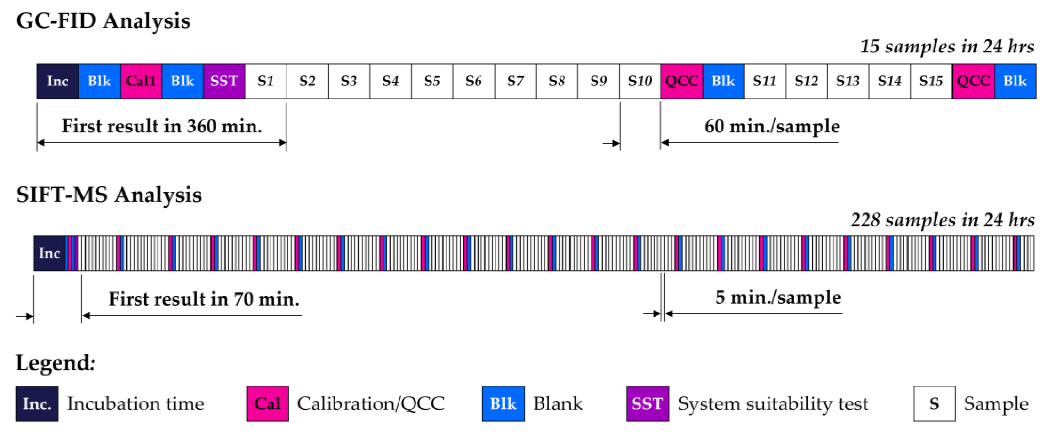
2.1. Automated SIFT-MS Analysis
2.2. Automated GC-FID Analysis
2.3. Sample Preparation and Analysis
3. Results
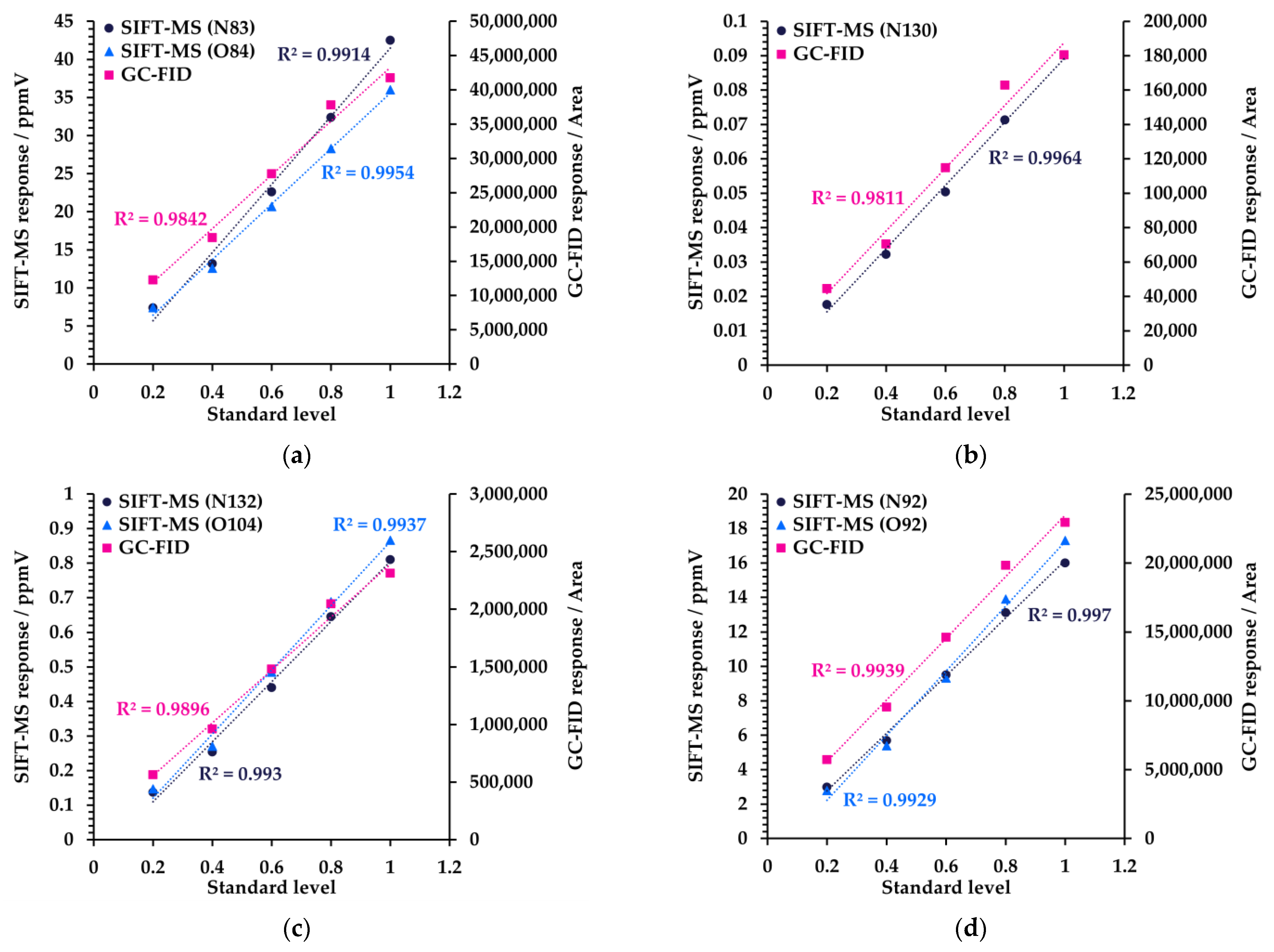
3.1. Linearity
3.2. Precision
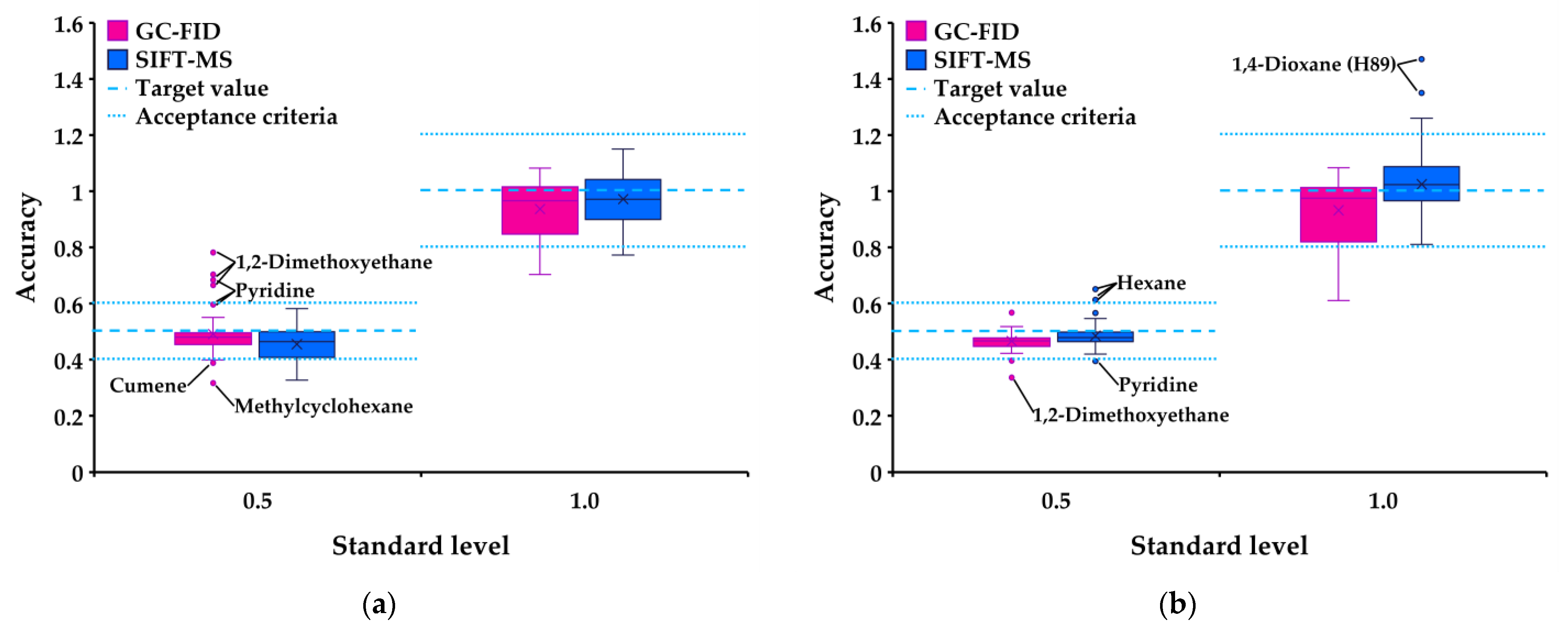
3.3. Accuracy
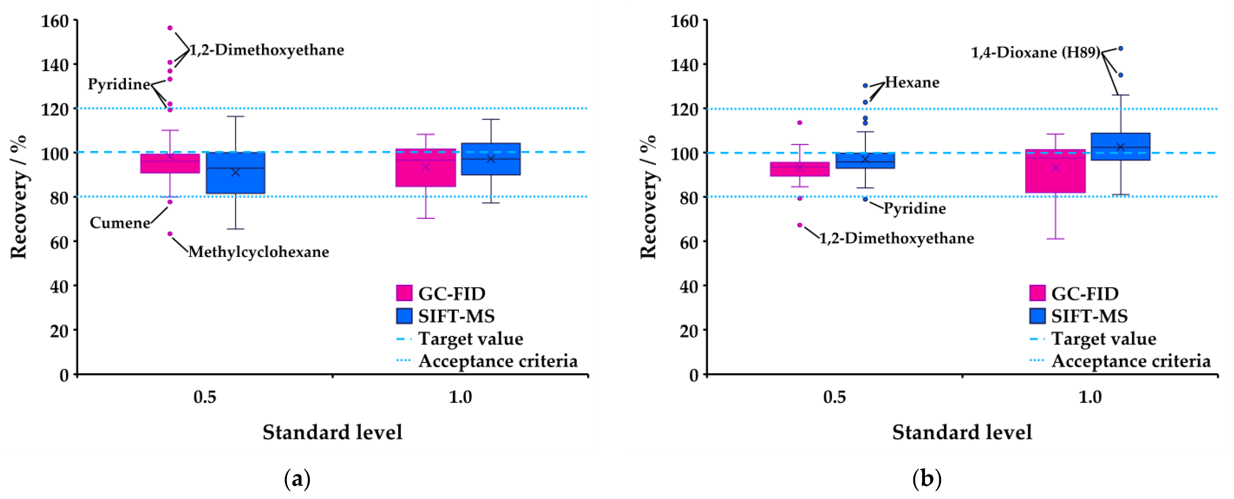
3.4. Recovery
4. Discussion
5. Conclusions
Supplementary Materials
Author Contributions
Funding
Institutional Review Board Statement
Informed Consent Statement
Data Availability Statement
Conflicts of Interest
References
- International Council for Harmonization of Technical Requirements for Pharmaceuticals for Human Use (ICH). Impurities: Guideline for Residual Solvents Q3C(R8). 2021. Available online: https://database.ich.org/sites/default/files/ICH_Q3C-R8_Guideline_Step4_2021_0422_1.pdf (accessed on 23 March 2023).
- United States Pharmacopeia. Residual Solvents 〈467〉; United States Pharmacopeia: Rockville, MD, USA, 2007. [Google Scholar]
- Residual Solvents—Verification of Compendial Procedures and Validation of Alternative Procedures 〈1467〉; United States Pharmacopeia: Rockville, MD, USA, 2019.
- Dai, L.; Quiroga, A.C.; Zhang, K.; Runes, H.B.; Yazzie, D.T.; Mistry, K.; Chetwyn, N.P.; Dong, M.W. A Generic Headspace GC Method for Residual Solvents in Pharmaceuticals: Benefits, Rationale, and Adaptations for New Chemical Entities. LCGC N. Am. 2010, 28, 54–66. Available online: https://www.researchgate.net/publication/281259692 (accessed on 23 March 2023).
- McEwan, M.J. Direct analysis mass spectrometry. In Ion Molecule Attachment Reactions: Mass Spectrometry; Fujii, T., Ed.; Springer: New York, NY, USA, 2015; pp. 263–317. [Google Scholar]
- Taylor, A.J.; Beauchamp, J.D.; Langford, V.S. Non-destructive and high-throughput—APCI-MS, PTR-MS and SIFT-MS as methods of choice for exploring flavor release. In Dynamic Flavor: Capturing Aroma Release Using Real-Time Mass Spectrometry; Beauchamp, J.D., Ed.; American Chemical Society: Washington, DC, USA, 2021; pp. 1–16. [Google Scholar] [CrossRef]
- Hastie, C.; Thompson, A.; Perkins, M.J.; Langford, V.S.; Eddleston, M.; Homer, N. Selected ion flow tube-mass spectrometry (SIFT-MS) as an alternative to gas chromatography/mass spectrometry (GC/MS) for the analysis of cyclohexanone and cyclohexanol in plasma. ACS Omega 2021, 6, 32818–32822. [Google Scholar] [CrossRef] [PubMed]
- Perkins, M.J.; Langford, V.S. Application of headspace-SIFT-MS to direct analysis of hazardous volatiles in drinking water. Environments 2022, 9, 124. [Google Scholar] [CrossRef]
- Perkins, M.J.; Langford, V.S. Multiple headspace extraction-selected ion flow tube mass spectrometry (MHE-SIFT-MS). Part 1: A protocol for method development and transfer to routine analysis. Rev. Sep. Sci. 2022, 4, e22001. [Google Scholar] [CrossRef]
- Smith, D.; Španěl, P.; Demarais, N.; Langford, V.S.; McEwan, M.J. Recent developments and applications of selected ion flow tube mass spectrometry (SIFT-MS). Mass Spec. Rev. 2023, e21835. [Google Scholar] [CrossRef]
- Langford, V.S. SIFT-MS: Quantifying the volatiles you smell … and the toxics you don’t. Chemosensors 2023, 11, 111. [Google Scholar] [CrossRef]
- Biba, E.; Perkins, M.J.; Langford, V.S. Stimuli to the Revision Process: High-Throughput Residual Solvent Analysis Using Selected Ion Flow Tube Mass Spectrometry (SIFT-MS). United States Pharmacopeia. Pharm. Forum 2021, 47, 1. Available online: https://online.usppf.com/usppf/document/GUID-2EE1BF6B-C82B-4F11-8E0B-C5520A4E8C3D_10101_en-US (accessed on 15 January 2023).
- Perkins, M.J.; Langford, V.S. Rapid Residual Solvent Analysis: Validation of an Alternative Procedure for USP Method 〈467〉 Using SIFT-MS. Syft Technologies Application Note. 2022. Available online: http://bit.ly/3Eq7Qx4 (accessed on 21 February 2023).
- Smith, D.; Španěl, P. Selected ion flow tube mass spectrometry (SIFT-MS) for on-line trace gas analysis. Mass Spec. Rev. 2005, 24, 661–700. [Google Scholar] [CrossRef]
- Hera, D.; Langford, V.S.; McEwan, M.J.; McKellar, T.I.; Milligan, D.B. Negative reagent ions for real time detection using SIFT-MS. Environments 2017, 4, 16. [Google Scholar] [CrossRef]
- Prince, B.J.; Milligan, D.B.; McEwan, M.J. Application of selected ion flow tube mass spectrometry to real-time atmospheric monitoring. Rapid Commun. Mass Spectrom. 2010, 24, 1763–1769. [Google Scholar] [CrossRef]
- Wagner, R.L.; Farren, N.J.; Davison, J.; Young, S.; Hopkins, J.R.; Lewis, A.C.; Carslaw, D.C.; Shaw, M.D. Application of a mobile laboratory using a selected-ion flow-tube mass spectrometer (SIFT-MS) for characterisation of volatile organic compounds and atmospheric trace gases. Atmos. Meas. Tech. 2021, 14, 6083–6100. [Google Scholar] [CrossRef]
- Španěl, P.; Smith, D. Selected ion flow tube studies of the reactions of H3O+, NO+, and O2+• with several amines and some other nitrogen-containing molecules. Int. J. Mass Spectrom. 1998, 176, 203–211. [Google Scholar] [CrossRef]
- Španěl, P.; Smith, D. Selected ion flow tube studies of the reactions of H3O+, NO+ and O2+• with several aromatic and aliphatic monosubstituted halocarbons. Int. J. Mass Spectrom. 1999, 189, 213–223. [Google Scholar] [CrossRef]
- Španěl, P.; Smith, D. Selected ion flow tube studies of the reactions of H3O+, NO+, and O2+• with some chloroalkanes and chloroalkenes. Int. J. Mass Spectrom. 1999, 184, 175–181. [Google Scholar] [CrossRef]
- Syft Technologies Limited. SIFT-MS Compound Library; Syft Technologies Limited: Christchurch, New Zealand, 2006. [Google Scholar]
- Syft Technologies Limited. SIFT-MS Compound Library; Syft Technologies Limited: Christchurch, New Zealand, 2014. [Google Scholar]
- Španěl, P.; Smith, D. SIFT studies of the reactions of H3O+, NO+, and O2+• with several ethers. Int. J. Mass Spectrom. Ion Proc. 1998, 172, 239–247. [Google Scholar] [CrossRef]
- Wang, T.; Španěl, P.; Smith, D. A selected ion flow tube study of the reactions of H3O+, NO+, and O2+• with several N- and O-containing heterocyclic compounds in support of SIFT-MS. Int. J. Mass Spectrom. 2004, 237, 167–174. [Google Scholar] [CrossRef]
- Syft Technologies Limited. SIFT-MS Compound Library; Syft Technologies Limited: Christchurch, New Zealand, 2013. [Google Scholar]
- Španěl, P.; Smith, D. SIFT studies of the reactions of H3O+, NO+, and O2+• with a series of alcohols. Int. J. Mass Spectrom. Ion Proc. 1997, 167–168, 375–388. [Google Scholar] [CrossRef]
- Španěl, P.; Ji, Y.; Smith, D. SIFT studies of the reactions of H3O+, NO+, and O2+• with a series of aldehydes and ketones. Int. J. Mass Spectrom. Ion Proc. 1997, 165–166, 25–37. [Google Scholar] [CrossRef]
- Midey, A.J.; Williams, S.; Miller, T.M.; Viggiano, A.A. Reactions of O2+•, NO+, and H3O+ with methylcyclohexane (C7H14) and cyclooctane (C8H16) from 298 to 700 K. Int. J. Mass Spectrom. 2003, 222, 413–430. [Google Scholar] [CrossRef]
- Dryahina, K.; Polasek, M.; Španěl, P. A selected ion flow tube, SIFT, study of the ion chemistry of H3O+, NO+, and O2+• ions with several nitroalkanes in the presence of water vapour. Int. J. Mass Spectrom. 2004, 239, 57–65. [Google Scholar] [CrossRef]
- Perkins, M.J. Unpublished Kinetic Data for Tetralin; Element Materials Technology: Cambridge, UK, 2018; Data available on request. [Google Scholar]
- Španěl, P.; Smith, D. SIFT studies of the reactions of H3O+, NO+ and O2+• with several aromatic and aliphatic hydrocarbons. Int. J. Mass Spectrom. 1998, 181, 1–10. [Google Scholar] [CrossRef]
- Perkins, M.J.; Langford, V.S. Application of routine analysis procedures to a direct mass spectrometry technique: Selected ion flow tube mass spectrometry (SIFT-MS). Rev. Sep. Sci. 2021, 3, e21003. [Google Scholar] [CrossRef]


| Parameters | Acceptance Criteria | Results: SIFT-MS | Results: GC-FID |
|---|---|---|---|
| Linearity | R2 > 0.90 | R2 ≥ 0.97 | R2 ≥ 0.94 |
| Precision: Repeatability | RSD is <20% 1 | 1.4–9.5%RSD | 2.0–16.9%RSD |
| Accuracy | <20% | ||
| 1. Tablet | |||
| a. 0.5 (50%) level | 0.4–0.6 | 0.404–0.511 | 0.424–0.519 |
| Exceptions: methylcyclohexane 0.387, pyridine 0.624, 1,2-dimethoxyethane 0.723 | |||
| b. 1.0 (100%) level | 0.8–1.2 | 0.844–1.126 | 0.819–1.079 |
| Exceptions: 1,4-dioxane 0.719, methanol 0.744, acetonitrile 0.799 | |||
| 2. Oral suspension | |||
| a. 0.5 (50%) level | 0.4–0.6 | 0.429–0.564 | 0.420–0.570 |
| Exceptions: 1,4-dioxane 1.002 (1 ion), hexane 0.627 | Exceptions: 1,2-dimethoxyethane 0.386 | ||
| b. 1.0 (100%) level | 0.8–1.2 | 0.883–1.134 | 0.893–1.079 |
| Exception: 1,4-dioxane 1.361 (1 ion) | Exceptions: 1,2-dimethoxyethane 0.769, methanol 0.771, 1,4-dioxane 0.772, MBK 0.792, acetonitrile 0.793, chloroform 0.796 | ||
| Recovery | 80–120% 2 | ||
| 1. Tablet | |||
| a. 0.5 (50%) level | 81.3–102.3% | 84.9–103.8% | |
| Exceptions: methylcyclohexane 77.5%, pyridine 124.8%, 1,2-dimethoxymethane 144.6% | |||
| b. 1.0 (100%) level | 84.4–112.6% | 89.4–107.9% | |
| Exceptions: 1,4-dioxane 71.9%, methanol 74.4%, acetonitrile 79.9% | |||
| 2. Oral suspension | |||
| a. 0.5 (50%) level | 85.8–112.8% | 84.0–114.1% | |
| Exceptions: hexane 125.4%, 1,4-dioxane 200.3% (1 ion) | Exceptions: 1,2-dimethoxyethane 77.2% | ||
| b. 1.0 (100%) level | 88.3–113.4% | 88.2–107.9% | |
| Exception: 1,4-dioxane 136.1% (1 ion) | Exceptions: 1,2-dimethoxymethane 76.9%, methanol 77.1%, 1,4-dioxane 77.2%, MBK 79.2%, chloroform 79.6%, acetonitrile 79.3% |
Disclaimer/Publisher’s Note: The statements, opinions and data contained in all publications are solely those of the individual author(s) and contributor(s) and not of MDPI and/or the editor(s). MDPI and/or the editor(s) disclaim responsibility for any injury to people or property resulting from any ideas, methods, instructions or products referred to in the content. |
© 2023 by the authors. Licensee MDPI, Basel, Switzerland. This article is an open access article distributed under the terms and conditions of the Creative Commons Attribution (CC BY) license (https://creativecommons.org/licenses/by/4.0/).
Share and Cite
Perkins, M.J.; Hastie, C.; Whitlock, S.E.; Langford, V.S. Pharmaceutical Residual Solvent Analysis: A Comparison of GC-FID and SIFT-MS Performance. AppliedChem 2023, 3, 290-302. https://doi.org/10.3390/appliedchem3020018
Perkins MJ, Hastie C, Whitlock SE, Langford VS. Pharmaceutical Residual Solvent Analysis: A Comparison of GC-FID and SIFT-MS Performance. AppliedChem. 2023; 3(2):290-302. https://doi.org/10.3390/appliedchem3020018
Chicago/Turabian StylePerkins, Mark J., Colin Hastie, Sophia E. Whitlock, and Vaughan S. Langford. 2023. "Pharmaceutical Residual Solvent Analysis: A Comparison of GC-FID and SIFT-MS Performance" AppliedChem 3, no. 2: 290-302. https://doi.org/10.3390/appliedchem3020018