Application of Back-Propagation Neural Network in the Post-Blast Re-Entry Time Prediction

Abstract

Predicting the post-blast re-entry time precisely can improve productivity and reduce accidents significantly. The empirical formulas for the time prediction are practical to implement, but lack accuracy. In this study, a novel method based on the back-propagation neural network (BPNN) was proposed to tackle the drawbacks. A numerical model was constructed and 300 points of sample data were recorded, with consideration to fresh air volume, occupational exposure limit, toxic gas volume per kg of explosives and roadway length. The BPNN model with six neurons in a hidden layer was then developed and prediction performance was discussed in terms of four indicators, namely, the root mean square error (RMSE), the coefficient of determination (R²), the mean absolute error (MAE) and the sum of squares error (SSE). Furthermore, one representative empirical formula was introduced and calibrated for the comparison. The obtained results showed that the BPNN model had a more remarkable performance, with RMSE of 21.45 (R²: 0.99, MAE: 10.78 and SSE: 40934), compared to the empirical formula, with RMSE of 76.89 (R²: 0.90, MAE: 42.06 and SSE: 526147). Hence, the BPNN model is a superior method for predicting the post-blast re-entry time. For better practical application, it was then embedded into the software.

1. Introduction

The number of underground mines is increasing due to the depletion of resources on the surface. The drill and blast (D&B) and tunnel boring machines (TBM) have been used in underground mines for excavation. Although TBM has been adopted at sites such as San Manual Mine and Stillwater Mine [1], many difficulties, including cutter wear and rock popping, etc., have hindered its development [2]. Consequently, D&B is still the main excavation method due to its flexibility and economy [3,4]. However, one of the shortcomings of D&B is that it emits a substantial amount of toxic gases, including carbon monoxide (CO), nitric oxide (NO) and nitrogen dioxide (NO₂). Among them, CO is the primary research object, due to its stability and large quantity [5]. For the purposes of improving cleaning efficiency and enhancing the production capacity, ventilation has been identified as one of the most effective methods and has been used widely [6].

The ventilation time taken to reduce the toxic gas concentration below the occupational exposure limit is defined as the post-blast re-entry time [5]. Additionally, a report has shown that most mines have more than four blasts per day, so estimating the post-blast re-entry time as accurately as possible will avoid the loss of significant amounts of production time [7]. Several methods have been studied and applied. For example, many mines have relied on the fixed-time interval to determine when the miners can re-enter the heading face to work continuously [8]. However, it should be noted that this may lead to a number of associated safety and health issues for workers. In order to improve accuracy, some empirical formulas were developed by using the flow balance, fitting the data obtained from numerical simulations, site tests, and laboratory experiments [4,7,9,10,11,12,13,14,15]. Despite the considerable advantages of empirical formulas, such as being simple, convenient, and timesaving, the calculation is less universal so that some parameters such as the dilution efficiency factor, need to be calibrated according to the particular mine where the concentration data can be monitored [15].

As opposed to the empirical formulas, artificial intelligence (AI) technologies have a good history of performance in prediction [16]. The technique has gained popularity in many fields, including UCS of rock [17,18], shear strength of rockfill material [19], backbreak in open-pit mines [20], ozone concentration [21] and carbon monoxide concentration [22]. Additionally, the AI technologies have the ability to consider several factors, and the results can be obtained directly based on the optimized AI model. AI can also avoid the above-mentioned limitations of the empirical formula. However, AI technologies have rarely been implemented into the re-entry time prediction, to the author’s knowledge.

Gathering reliable sample data is necessary for the construction of AI models [23]. Field data is of course the most reliable type, but one that is not easy to access, due to the harsh environment in the mines [24]. On the contrary side, numerical simulation has gained worldwide attention in the study of the migration behaviors of blasting production in the underground roadway, owing to the superiority of visualization, data richness and ease of operation [25,26,27,28]. However, the length of these models is typically short, as numerical simulation requires a high level of computational performance, especially for long roadways with a significant amount of nodes. The Ventsim software, which is based on the Hardy Cross algorithm, and which has been used to study the post-blast re-entry time in some complex roadways with affordable computation time [15,29], was thus selected to calculate the time under various conditions in this study.

Therefore, this paper aims to develop a BPNN model for predicting the post-blast re-entry time. The rest of this study is organized as follows. The section titled “Model process and data preparation” introduces the construction of models used, as well as the process of database establishment, including the selection and analysis of parameter ranges. The section titled “Methodology” describes the algorithm of BPNN as well as the process of calibrating the empirical formula in detail, in addition to four indicators adopted to evaluate the performance of proposed models. The section titled “Results and discussions” contains the description of building the architecture of the BPNN and a performance comparison of both models for the time prediction. The section titled “Algorithm embedding” exhibits one software developed based on the proposed models. In the last section, the main conclusions and future development are given.

2. Model Process and Data Preparation

2.1. Model Construction

The research object is one cross-section of the roadway at a depth of approximately 580 m below the surface. The section’s size and its corresponding 3-D model constructed in Ventsim are shown in Figure 1. It is a three-core arch structure with an area of 14.04 m². The width, wall height and arch height are 3.95 m, 2.8 m and 0.95 m, respectively. Facilities such as cables and supports inside the roadway were not taken into consideration. The amount of explosives used each time are about 40 kg and the temperature is around 300 K. It is worth pointing out that the ventilation duct was placed off the roadway in this software for the convenience of real-time viewing of ventilation performance.

2.2. Database Generation

Four parameters, namely, average velocity within the roadway, occupational exposure limit, toxic gas volume per kg of explosives and length of roadway, have frequently been considered when calculating the relevant time [11,15]. Hence, these four parameters were also used for developing the BPNN model in this study. Due to the fact that the fresh-air volume of the ventilation duct has a considerable impact on the average velocity within the roadway, the minimal average velocity in the excavation roadway was set at 0.25 m/s and the highest average velocity was set at 4 m/s in the mining area, given in the safety regulations for metal and nonmetal mines of China [30]. As a consequence, the average velocity ranged from 0.25 m/s to 4 m/s in this study. Moreover, some indexes for assessing occupational exposure limit have been proposed, depending upon the actual requirements. For example, time weight average (TWA) is defined as the average permissible concentration within a normal 8 h workday and 40 h work-week. Short term exposure limit (STEL) considers the permissible concentration limit for up to 15 min with the serious implementation of the TWA.

Table 1. Occupational exposure limit for CO in different countries [13].

	TWA/ppm	STEL/ppm
ASM-2	50	100
NIOSH REL	35	200
NOHSC	30	200
OSHA PEL	35	200
CHINA	16	24

Note: ASM-2 is Instructions Technique Complementary to Mining Safety Actions (Spain); NIOSH is the National Institute for Occupational Safety and Health; NOHSC is the National Occupational Health and Safety Commission; OSHA is the Occupational Safety and Health Administration.

shows the TWA and STEL of different countries for CO. It can be seen that China has the strictest regulations for exposure concentration, so 24 ppm was used as the monitoring standard rather than the 16 ppm level found in some regulations [31]. Taking all of the above factors into account, the occupational exposure limits in this study were taken to be between 24 ppm and 50 ppm, in order to meet a variety of requirements.

Toxic gas production is susceptible to a variety of influencing factors, such as the sort of explosives [32], the environment of the roadway [33], the type of blasting design, the method of detonation, and so on [34]. Therefore, the amount of toxic gases produced in each detonation varies slightly. The #2 rock emulsion explosive was adopted in this study. The toxic gas volume per kg of explosives in the underground roadway is from 36 L/kg to 42 L/kg, as given by Wang [35]. In addition, the length of the roadway is increased with the continuous construction of excavation engineering. Herein, the range from 200 m up to 1500 m was studied. Figure 2 presents the minimum, lower quartile, median, upper quartile and maximum for each parameter in boxplots. It illustrates that each parameter shows a uniform distribution.

A total of 300 input samples were generated based on the ranges mentioned above, and then these models with specific parameter values were constructed and simulated in Ventsim software to predict the post-blast re-entry time. In total, 300 pieces of data were archived herein as described in Appendix A. The correlation matrix of the dataset is presented in Figure 3. The distributions and correlation coefficients for any two parameters are presented in the lower and upper of this figure, respectively. For the lower, it is clear that the relationship between the inputs and outputs is nonlinear where only the relationship of velocity versus time reveals a distribution similar to a negative exponential. For the upper, the darker the blue, the stronger the negative correlation. Conversely, the lighter the red, the weaker the positive correlation. As can be observed, the correlation coefficient between the four input parameters is low, as they are independent of each other. Additionally, both length and velocity show statistically significant relationships with the time, after significance tests. Despite the fact that gas and limit have lower correlation coefficients, these parameters still remain valid for the subsequent comparative analysis with the empirical formula.

3. Methodology

3.1. BPNN Algorithm

BPNN is a classical supervised learning method fusing the feedforward neural network and the back-propagation algorithm. It has been used in many fields and achieved excellent performance because of its capabilities of outstanding nonlinear fitting and generalization. For instance, Li et al. [23] have successfully used a BPNN model to predict the stress values when evaluating pillar stability. Zhao et al. [36] applied an integrated model based on the traditional BPNN to predict air pollution concentration and demonstrated that the method is more practical. Hence, BPNN was chosen in this study for predicting the post-blast re-entry time. There are five steps, namely, initialization of weights and biases, feedforward propagation of data, back-propagation of error, optimization of weights and biases and judgment of termination conditions.

At first, weights w and biases θ at the hidden layer and output layer are initialized with random numbers. The magnitude of each weight stands for the degree of influence of the connected neurons on the output, while the bias represents the level of difficulty in generating activation. After that, the accumulation of y_j in the hidden layer and z_k in the output layer can be calculated by the following formulas, respectively:

$$y_j=f\left({\displaystyle \sum _{i=1}^n\left(w_{ij}\times x_i\right)-{\theta }_j}\right) (i=1,2,\cdots n;j=1,2,\cdots m)$$

(1)

$$z_k=f\left({\displaystyle \sum _{j=1}^m\left(w_{jk}\times y_j\right)-{\theta }_k}\right) (j=1,2,\cdots m;k=1,2,\cdots l)$$

(2)

where f is an activation function; x, y and z are the output values of the input layer, hidden layer and output layer, respectively; and n, m and l represent the number of neurons at the input layer, hidden layer and output layer, respectively.

Afterward, the back-propagation is performed. The neuron error in the hidden layer and the output layer are E_j and E_k, respectively. As the error is the functions of weights, the tuning weights ∆w_ij between the input layer and the hidden layer as well as the tuning weights ∆w_jk between the hidden layer and the output layer are as follows:

$$\Delta w_{ij}=-\eta \frac{\partial E_j}{\partial w_{ij}}$$

(3)

$$\Delta w_{jk}=-\eta \frac{\partial E_k}{\partial w_{jk}}$$

(4)

where η is the learning rate.

Subsequently, the updated weights w_ij (t + 1) and w_jk (t + 1) are given as:

$$w_{ij}(t+1)=w_{ij}(t)+\Delta w_{ij}$$

(5)

$$w_{jk}(t+1)=w_{jk}(t)+\Delta w_{jk}$$

(6)

where t represents the number of iterations.

Finally, the process of training is conducted until the convergence conditions are satisfied, or otherwise, these steps (except for the initialization) are looped. In total, the framework of this research based on the BPNN model can be found in Figure 4.

3.2. Calibrating Empirical Formula

The schematic of ventilation in the longitudinal profile of the roadway is presented in Figure 5. It is given that the length of the working area and roadway are L₀ and L, respectively. The area of roadway is S. The fresh air volume discharged from the ventilation duct is Q and the toxic gases concentration uniformly distributed in the working area of volume V is C₀ at the initial moment. According to the flow balance, the amount of toxic gases removed after $\Delta t$ time of ventilation is Q × $\Delta t$. Hence, the concentration C after T time of ventilation can be calculated by the following:

$$C=\underset{n\to \propto }{lim}{C}_0{(\frac{V-Q\Delta t}{V})}^n=\underset{\Delta t\to 0}{lim}{C}_0{(1-\frac{Q\Delta t}{V})}^{\frac{T}{\Delta t}}=C_0{e}^{-\frac{TQ}{V}}$$

(7)

where n is the ratio of T to $\Delta t$.

Moreover, Equation (7) can be further written by taking the logarithm as:

$$T=\frac{V}{Q}\ln \frac{C_0}{C}$$

(8)

Furthermore, some other empirical formulas shown in

Table 2. Empirical formulas for time prediction.

Reference	Equation	Way
[4]	$C=\frac{V_G}{2A\sqrt{\mathsf{\pi }DT}}{e}^{\left(\frac{-{(L-uT)}^2}{4DT}\right)}$	Calibration
[7]	$T=e^{-\left(\frac{Q-60.119}{12.924}\right)}$	Calibration
[7]	$T=2383.7Q^{-1.574}$	Calibration
[9]	$C=p_1{T}_n+p_2{T}_{n-1}+\cdots +p_{n}T+p_{n+1}$	Fitting
[9]	$C=1048e^{-{\left(\frac{T-6.464}{0.8676}\right)}^2}$	Fitting
[10]	$T=13.118e^{0.0017L}$	Fitting
[11]	$T=n\ln \left(\frac{C}{C_T}\right)$	Derivation
[11]	$T=\frac{V}{Q+Q_g}\ln \left[\frac{\left(Q_g+Q{B}_g\right)-\left(Q+Q_g\right)C}{\left(Q_g+Q{B}_g\right)-\left(Q+Q_g\right)C_T}\right]$	Derivation
[15]	$T=\frac{V_w}{Q\times f_d}\ln \left(\frac{C}{C_T}\right)$	Calibration

Note: T: ventilation time required, min or s; Q: fresh air quantity, m³/s; C: gas concentration at the beginning of ventilation, ppm; p_1, p₂, …, p_n+1: fitting constants; V_W: volume of working space, m³; f_d: dilution efficiency factor; C_T: gas concentration at time T, ppm; V_G: volume of gas at the heading and beginning of time, m³; A: area of cross-section of roadway, m²; D: effective axial dispersion factor, m²/s; L: distance away from the heading, m; u: average air velocity, m/s; n: numbers of fresh air which is passing through the working space; Q_g: inflow rate of the toxic gases, m³/s; and B_g: concentration of toxic gases in the ventilation duct, %.

have been developed by using different techniques such as mathematical derivation, data fitting and formula calibration. Among them, the empirical formula given by [15] was selected for comparison with the BPNN model because it provides some optimization based on Equation (8) and is more representative than others.

To acquire dilution efficiency factor f_d in the formula given by [15], the sample with the post-blast re-entry time of 86 s, velocity of 3.79 m/s, length of 474 m, gas production of 36.2 L/kg and exposure limit value of 34 ppm was randomly picked. Some other parameters, namely the working space Vw, fresh air quantity Q and gas concentration C need to be calculated as follows, respectively:

$$V_w=\frac{G\times b}{x_0}$$

(9)

$$Q=u\times A$$

(10)

$$C=\frac{28\times G\times b}{29\times l\times A-G\times b}$$

(11)

$$l=15+\frac{G}{5}$$

(12)

where G is the mass of the explosive, kg; b is the toxic gas volume per kg of explosives, m³/kg; x₀ is the peak concentration of gas at the entrance monitored, ppm; and l is the throwing distance of toxic gas, m.

After that, the dilution efficiency factor of 0.73 can be obtained. The final empirical formula, which was employed to calculate the post-blast re-entry time and then compared to the BPNN, is given below:

$$T=\frac{V_w}{0.73Q}\ln \left(\frac{C}{C_T}\right)$$

(13)

3.3. Performance Indicators for the Assessment of Models

Four performance indicators, the root mean square error (RMSE), the coefficient of determination (R²), the mean absolute error (MAE) and the sum of squares error (SSE) were chosen to evaluate the performance of the models developed in this study [37]. Among them, RMSE is taken to measure the deviation between the actual value and the predicted value, where the smaller the value, the better the model’s performance. R² is available to represent the goodness of fit of the model to the sample data. The closer it is to 1, the stronger the fit is. MAE can reflect the extent of actual prediction error, with smaller values indicating that the prediction is closer to the actual value. SSE is the accumulation of squared error between the predicted value and the actual value. A larger value means a worse quality model when the number of samples is the same. They are defined by the following:

$$\mathrm{RMSE}=\sqrt{\frac{1}{n}{\displaystyle \sum _{i=1}^n{(Tim{e}_{o,i}-Tim{e}_{p,i})}^2}}$$

(14)

$${\mathrm{R}}^2=1-\frac{{\displaystyle \sum _{i=1}^n{(Tim{e}_{o,i}-Tim{e}_{p,i})}^2}}{{\displaystyle \sum _{i=1}^n{(Tim{e}_{o,i}-\overline{Tim{e}_o})}^2}}$$

(15)

$$\mathrm{MAE}=\frac{1}{n}{\displaystyle \sum _{i=1}^n|Tim{e}_{o,i}-Tim{e}_{p,i}|}$$

(16)

$$\mathrm{SSE}={\displaystyle \sum _{i=1}^n{(Tim{e}_{o,i}-Tim{e}_{p,i})}^2}$$

(17)

where n is the number of samples; Time_o,i, Time_p,i are the post-blast re-entry time of actual value and the predicted value, respectively; and $\overline{Tim{e}_o}$ represents the mean value of actual post-blast re-entry time.

4. Results and Discussion

4.1. Building the Architecture of the BPNN

An excellent BPNN model, one which has the best weights obtained from the training phase, can predict the post-blast re-entry time precisely. In this study, the BPNN model built on MATLAB was trained and tested with 210 samples (70%) and 90 samples (30%), respectively. The changes in RMSE and R² were recorded while the model had a different number of neurons at the hidden layer, as shown in

Table 3. Performance of BPNN models with different numbers of neurons in the hidden layer.

Model	Neurons	RMSE		R2
		Training	Testing	Training	Testing
1	2	16.0196	21.9249	0.9959	0.9922
2	3	55.9012	37.0202	0.9502	0.9776
3	4	72.4646	60.601	0.9163	0.9401
4	5	61.6996	50.5617	0.9393	0.9583
5	6	12.6171	21.3421	0.9975	0.9926
6	7	14.3551	21.026	0.9967	0.9928
7	8	14.7677	21.4577	0.9965	0.9925
8	9	14.2703	22.0516	0.9968	0.9921
9	10	13.1419	21.6439	0.9973	0.9924

Note: the line in bold type indicates the best model.

. It can be summarized that the model with six neurons in the hidden layer performed best in which the lowest RMSE of 12.6171 and the highest R² of 0.9975 can be acquired. At the same time, it also has a remarkable performance in the testing phase. Hence, this model was served as the final post-blast re-entry time prediction model and the schematic diagram is presented in Figure 6.

4.2. Performance Comparison between BPNN and Formula

The BPNN and empirical formula previously developed were run to predict the post-blast re-entry time in the training set and the test set. The models’ performance, including RMSE, R², MAE and SSE, was summarized in

Table 4. Performance comparison of both models.

Indicators	Training		Testing
	Empirical	BPNN	Empirical	BPNN
RMSE	61.81	12.61	76.89	21.34
MAE	38.34	7.66	42.06	10.78
R2	0.94	0.99	0.90	0.99
SSE	798352	33429	526147	40934

. As can be seen in this table, the BPNN model has a better performance in both the training set and the test set than does the empirical formula. The average prediction error of BPNN in the test set is only 10.78 s, which is approximately a quarter of the empirical formula. Additionally, the goodness of fit of BPNN is closer to 1, indicating that it can better account for the relationship between the inputs and output than can the empirical formula. It should be noted that the delay caused by the empirical formula each time will accumulate with the increasing number of detonations. To reduce the losses, the BPNN model should be adapted to predict the post-blast re-entry time.

In order to compare the performance of both models more exactly, the regression diagrams in the training phase and the testing phase are described in Figure 7. The horizontal axes represent the actual time. The vertical axes render the prediction value obtained from the BPNN and the empirical formula. The slope of diagonal lines with the black color is 1. Other radical lines with deviations of 10% and 30% from the diagonal lines are also drawn in this diagram. Taken as a whole, the BPNN model has a higher accuracy than does the empirical formula in both sets, because the data points are closer to the diagonal line, whereas some data points obtained from the empirical formula are far outside of the line of 30%, especially in the testing phase. It can also be seen that most of them are larger than the actual time when the ventilation time required is larger than 400 s. At the same time, the BPNN in the testing phase has a larger error than in the training phase, but these data points are almost limited to the radical line of 10%. Hence, the BPNN model can offer more stable performance and more accurate results.

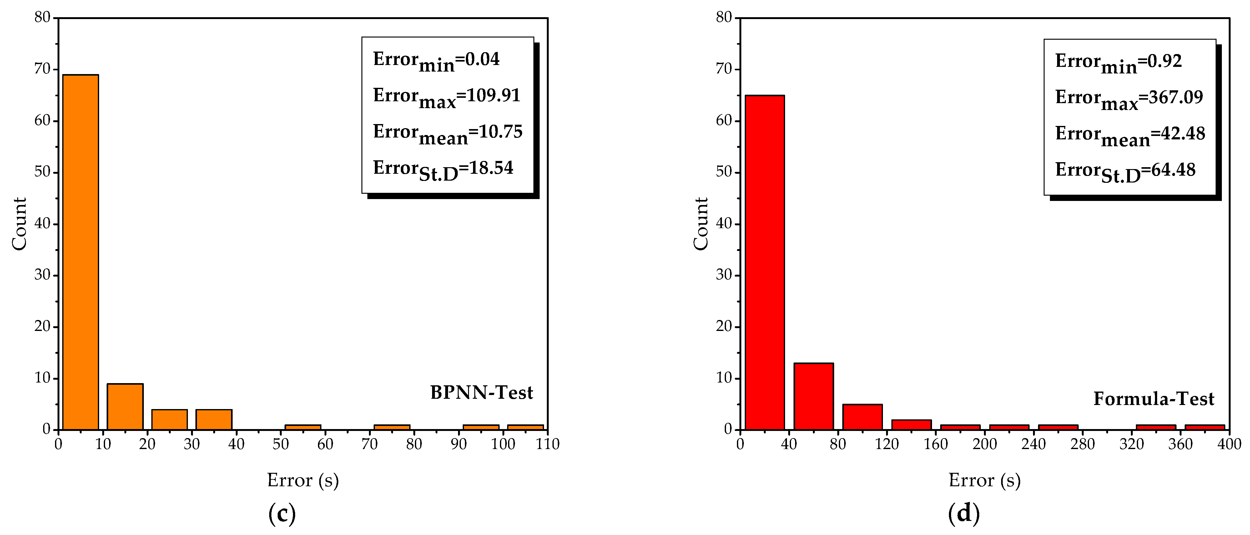
Figure 8 illustrates the error distributions of both models in the training phase and testing phase and some statistical indicators, i.e., the minimum of error (Error_min), the maximum of error (Error_max), the mean of error (Error_mean) and the standard deviation of error (Error_St.D) are contained in this figure as criteria. The horizontal axes represent the error values between the actual time and the predicted time. The vertical axes are the count within a specified error range. Accordingly, the higher the error bar near the origin and the lower the statistical indicators are, the smaller the model error. As can be realized, the BPNN shows promising results because the region of horizontal axes of the first bar is only from 0 to 10 in the BPNN model when the count of the first bar is almost equal in both models. Additionally, it can be observed that the empirical formula has similar performance in both the training phase and the testing phase.

5. Algorithm Embedding

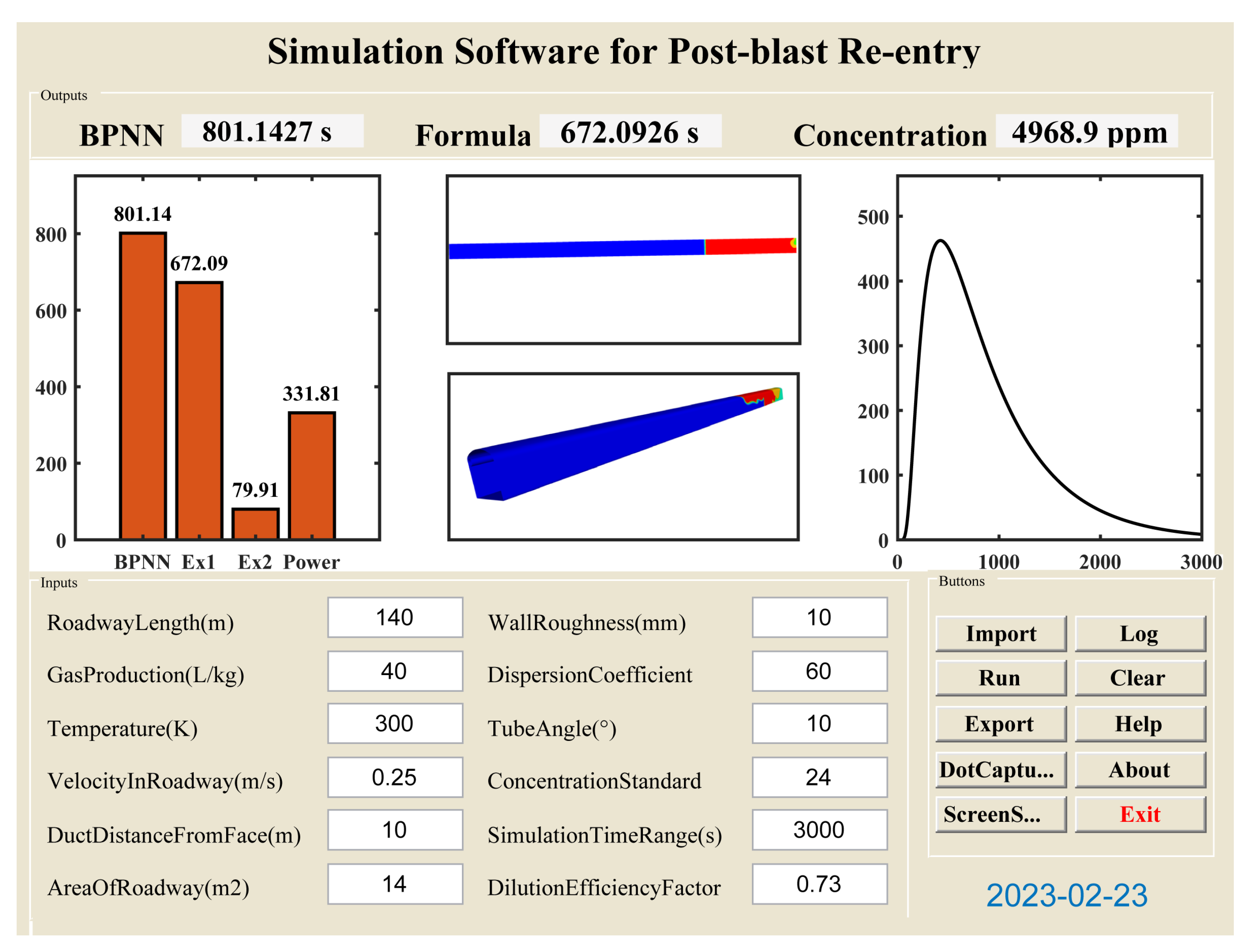
Given the complicated environment on the site and the inconvenience of running code in the engineering practice, some scientists have performed a lot of work on the application of construction schedule methods, such as the use of software. Song et al. [38] developed a universal engineering construction system simulation software for the construction schedule visualization simulation of hydraulics and hydropower. Wang et al. [10] embedded a ventilation time function in existing software to replace the empirical values for the construction processes and schedule arrangement. In this study, the trained BPNN model was embedded into an existing software module named Simulation Software for Post-blast Re-entry to enhance the performance and facilitate practical use in the central control room located on the surface (see Figure 9). It can be seen that the prediction time obtained from the BPNN model is displayed as both numeric and bar values. Additionally, some optimizations have been applied to the software based on this study. For example, the standard concentration can be input more flexibly according to the requirements rather than using the fixed one. The dilution efficiency factor in the empirical formula was also appended to this software to provide more reference information for users in the period of decision-making. Furthermore, the software can also be utilized to support the formulation of a preliminary schedule. To respond to the call to develop an intelligent mine, interfacing with the mine’s integrated system will be the object in future research.

6. Conclusions

Determining the post-blast re-entry time is essential in the excavation field of tunnel and mining to prevent the occurrence of poisoning and asphyxiation incidents. In this paper, a BPNN model was proposed with consideration of four parameters most used in former studies. An empirical formula was calibrated to compare the performance with the proposed BPNN model. It found that the BPNN model with six neurons in the hidden layer outperforms the others. Furthermore, the results show that the BPNN model has a higher reliability and accuracy (RMSE: 21.45; R²: 0.99; MAE: 10.78; SSE: 40934) compared with the empirical formula (RMSE: 76.89; R²: 0.90; MAE: 42.06; SSE: 526147). In order to facilitate the engineering use of the BPNN model developed in this study, the model has been embedded in one software application. The operator can not only set schedules for production tasks in advance but also can perform some ventilation optimization by adjusting parameters in this software to facilitate the cleaning efficiency of toxic gases.

This study provides an effective tool for the prediction of post-blast re-entry time in excavation engineering. However, some other influence factors, such as the temperature and the interactions between the wall roughness and the velocity of airflow, etc., may also affect the results; a fact which should be considered to achieve a better agreement between the predicted results and the actual situations. This will be discussed in future research.

References

- Cigla, M.; Yagiz, S.; Ozdemir, L. Application of tunnel boring machines in underground mine development. In Proceedings of the International Mining Congress and Exhibition, Turkey, Ankara, 19–22 June 2001. [Google Scholar]
- Zheng, Y.L.; Zhang, Q.B.; Zhao, J. Challenges and opportunities of using tunnel boring machines in mining. Tunn. Undergr. Space Technol. 2016, 57, 287–299. [Google Scholar] [CrossRef]
- Pu, Q.; Luo, Y.; Huang, J.; Zhu, Y.; Hu, S.; Pei, C.; Zhang, G.; Li, X. Simulation study on the effect of forced ventilation in tunnel under single-head drilling and blasting. Shock. Vib. 2020, 2020, 8857947. [Google Scholar] [CrossRef]
- Bahrami, D.; Yuan, L.; Rowland, J.H.; Zhou, L.; Thomas, R. Evaluation of post-blast re-entry times based on gas monitoring of return air. Min. Metall. Explor. 2019, 36, 513–521. [Google Scholar] [CrossRef]
- Menéndez, J.; Merlé, N.; Fernández-Oro, J.M.; Galdo, M.; de Prado, L.Á.; Loredo, J.; Bernardo-Sánchez, A. Concentration, propagation and dilution of toxic gases in underground excavations under different ventilation modes. Int. J. Environ. Res. Public Health 2022, 19, 7092. [Google Scholar] [CrossRef]
- Chen, J.; Qiu, W.; Rai, P.; Ai, X. Emission characteristics of CO and NOx from tunnel blast design models: A comparative study. Pol. J. Environ. Stud. 2021, 30, 5503–5517. [Google Scholar] [CrossRef]
- Gillies, A.D.S.; Wu, H.W.; Shires, D. Development of an assessment tool to minimize safe after blast re-entry time to improve the mining cycle. In Proceedings of the Tenth US/North American Mine Ventilation Symposium, Anchorage, AK, USA, 16–19 May 2004. [Google Scholar]
- De Souza, E. Procedures for mitigating safety risks associated with post-blast re-entry times. CIM J. 2023, 14, 2–10. [Google Scholar] [CrossRef]
- Torno, S.; Torano, J.; Ulecia, M.; Allende, C. Conventional and numerical models of blasting gas behaviour in auxiliary ventilation of mining headings. Tunn. Undergr. Space Technol. 2013, 34, 73–81. [Google Scholar] [CrossRef]
- Wang, X.L.; Liu, X.P.; Sun, Y.F.; An, J.; Zhang, J.; Chen, H.C. Construction schedule simulation of a diversion tunnel based on the optimized ventilation time. J. Hazard. Mater. 2009, 165, 933–943. [Google Scholar] [CrossRef]
- Souza, E.D.; Katsabanis, P.D. On the prediction of blasting toxic fumes and dilution ventilation. Eng. Geol. 1991, 13, 223–235. [Google Scholar] [CrossRef]
- Hebda-Sobkowicz, J.; Gola, S.; Zimroz, R.; Wylomanska, A. Identification and statistical analysis of impulse-like patterns of carbon monoxide variation in deep underground mines associated with the blasting procedure. Sensors 2019, 19, 2757. [Google Scholar] [CrossRef] [Green Version]
- Torno, S.; Toraño, J. On the prediction of toxic fumes from underground blasting operations and dilution ventilation. Conventional and numerical models. Tunn. Undergr. Space Technol. 2020, 96, 103194. [Google Scholar] [CrossRef]
- Zhou, Y.; Yang, Y.; Bu, R.W.; Ma, F.; Shen, Y.J. Effect of press-in ventilation technology on pollutant transport in a railway tunnel under construction. J. Clean. Prod. 2020, 243, 118590. [Google Scholar] [CrossRef]
- Stewart, C.M. Practical prediction of blast fume clearance and workplace re-entry times in development headings. In Proceedings of the 10th International Mine Ventilation Congress, Sun City, South Africa, 2–8 August 2014. [Google Scholar]
- Li, C.Q.; Zhou, J.; Armaghani, D.J.; Cao, W.Z.; Yagiz, S. Stochastic assessment of hard rock pillar stability based on the geological strength index system. Geomech. Geophys. Geo-Energy Geo-Resour. 2021, 7, 47. [Google Scholar] [CrossRef]
- Li, J.; Li, C.; Zhang, S. Application of six metaheuristic optimization algorithms and random forest in the uniaxial compressive strength of rock prediction. Appl. Soft Comput. 2022, 131, 109729. [Google Scholar] [CrossRef]
- Li, C.; Zhou, J.; Dias, D.; Gui, Y. A kernel extreme learning machine-grey wolf optimizer (KELM-GWO) model to predict uniaxial compressive strength of rock. Appl. Sci. 2022, 12, 8468. [Google Scholar] [CrossRef]
- Zhou, J.; Li, E.; Wei, H.; Li, C.; Qiao, Q.; Armaghani, D.J. Random forests and cubist algorithms for predicting shear strengths of rockfill materials. Appl. Sci. 2019, 9, 1621. [Google Scholar] [CrossRef] [Green Version]
- Li, C.; Zhou, J.; Khandelwal, M.; Zhang, X.; Monjezi, M.; Qiu, Y. Six novel hybrid extreme learning machine–swarm intelligence optimization (ELM–SIO) models for predicting backbreak in open-pit blasting. Nat. Resour. Res. 2022, 31, 3017–3039. [Google Scholar] [CrossRef]
- Eslami, E.; Choi, Y.; Lops, Y.; Sayeed, A. A real-time hourly ozone prediction system using deep convolutional neural network. Neural Comput. Appl. 2019, 32, 8783–8797. [Google Scholar] [CrossRef] [Green Version]
- Wang, Y.; Liu, P.; Xu, C.; Peng, C.; Wu, J. A deep learning approach to real-time CO concentration prediction at signalized intersection. Atmos. Pollut. Res. 2020, 11, 1370–1378. [Google Scholar] [CrossRef]
- Li, C.Q.; Zhou, J.; Armaghani, D.J.; Li, X.B. Stability analysis of underground mine hard rock pillars via combination of finite difference methods, neural networks, and Monte Carlo simulation techniques. Undergr. Space 2021, 6, 379–395. [Google Scholar] [CrossRef]
- Huang, R.Y.; Shen, X.; Wang, B.; Liao, X. Migration characteristics of CO under forced ventilation after excavation roadway blasting: A case study in a plateau mine. J. Clean. Prod. 2020, 267, 122094. [Google Scholar] [CrossRef]
- Chang, P.; Xu, G.; Zhou, F.; Mullins, B.J.; Abishek, S.; Chalmers, D. Minimizing DPM pollution in an underground mine by optimizing auxiliary ventilation systems using CFD. Tunn. Undergr. Space Technol. 2019, 87, 112–121. [Google Scholar] [CrossRef]
- Toraño, J.; Torno, S.; Menéndez, M.; Gent, M.R.; Velasco, J. Models of methane behaviour in auxiliary ventilation of underground coal mining. Int. J. Coal Geol. 2009, 80, 35–43. [Google Scholar] [CrossRef]
- Wei, N.; Zhong-an, J.; Dong-mei, T. Numerical simulation of the factors influencing dust in drilling tunnels: Its application. Min. Sci. Technol. (China) 2011, 21, 11–15. [Google Scholar] [CrossRef]
- Zhang, H.; Sun, J.; Lin, F.; Chen, S.; Yang, J. Optimization scheme for construction ventilation in large-scale underground oil storage caverns. Appl. Sci. 2018, 8, 1952. [Google Scholar] [CrossRef] [Green Version]
- Bismark, A.; Opafunso, Z.O.; Oniyide, G.O. Predicting the re-entry time at Chirano Gold Mine limited southwestern Ghana using ventsim simulation software. Niger. J. Eng. 2022, 29, 102–112. [Google Scholar]
- GB 16423-2020Safety Regulation for Metal and Nonmetal Mines; Ministry of Emergency Management of the People’s Republic of China: Beijing, China; Emergency Management Press: Beijing, China, 2020.
- AQ 2031-2011Regulations for The Construction of Monitoring and Supervision System in Metal and Nonmetal Underground Mine; Ministry of Emergency Management of the People’s Republic of China: Beijing, China; China Coal Industry Publishing House: Beijing, China, 2011.
- Zawadzka-Małota, I. Testing of mining explosives with regard to the content of carbon oxides and nitrogen oxides in their detonation products. J. Sustain. Min. 2015, 14, 173–178. [Google Scholar] [CrossRef] [Green Version]
- Brake, D.J. A review of good practice standards and re-entry procedures after blasting and gas detection generally in underground hardrock mines. In Proceedings of the 15th North American Mine Ventilation Symposium, Blacksburg, VA, USA, 21–23 June 2015; pp. 20–25. [Google Scholar]
- Wang, Y.M. Mine Ventilation and Dust Control; Metallurgical Industry Press: Beijing, China, 1993; p. 198. [Google Scholar]
- Wang, X.G. Emulsion Explosives, 2nd ed.; Metallurgical Industry Press: Beijing, China, 2008; p. 575. [Google Scholar]
- Zhao, H.; Wang, Y.J.; Song, J.; Gao, G. The pollutant concentration prediction model of NNP-BPNN based on the INI algorithm, AW method and neighbor-PCA. J. Ambient. Intell. Hum. Comput. 2018, 10, 3059–3065. [Google Scholar] [CrossRef]
- Zhang, J.; Dias, D.; An, L.; Li, C. Applying a novel slime mould algorithm-based artificial neural network to predict the settlement of a single footing on a soft soil reinforced by rigid inclusions. Mech. Adv. Mater. Struct. 2022, 1–16. [Google Scholar] [CrossRef]
- Song, Y.; Zhong, D.H. Study on construction schedule management and control method for hydraulic & hydropower engineering based on visual simulation. Syst. Eng.-Theory Pract. 2006, 8, 55–62. [Google Scholar] [CrossRef]
Figure 1.
Geometry of researched model.
Figure 2.
Boxplots of input parameters.
Figure 3.
Correlation between input and output parameters.
Figure 4.
Flowchart of the research process.
Figure 5.
Schematic of ventilation.
Figure 6.
Proposed BPNN model for predicting time.
Figure 7.
Regression diagrams of both models in the training and testing phase: (a) BPNN in training phase; (b) empirical formula in training phase; (c) BPNN in testing phase; and (d) empirical formula in testing phase.
Figure 8.
Prediction error comparison of both models in the training and testing phase: (a) BPNN in training phase; (b) empirical formula in training phase; (c) BPNN in testing phase; and (d) empirical formula in testing phase.
Figure 9.
Interface of simulation software for predicting time.